High order parametric polynomial approximation of conic sections Gaˇsper Jakliˇc a,b,c , Jernej Kozak a,b , Marjeta Krajnc a,b , a,b,∗ ˇ Vito Vitrih c , Emil Zagar a FMF,
University of Ljubljana, Jadranska 19, Ljubljana, Slovenia b IMFM,
c PINT,
Jadranska 19, Ljubljana, Slovenia
University of Primorska, Muzejski trg 2, Koper, Slovenia
Abstract In this paper, a particular shape preserving parametric polynomial approximation of conic sections is studied. The approach is based upon a general strategy to the parametric approximation of implicitly defined planar curves. Polynomial approximants derived are given in a closed form and provide the highest possible approximation order. Although they are primarily studied to be of practical use, their theoretical background is not to be underestimated: they confirm the H¨ollig-Koch’s conjecture for the Lagrange interpolation of conic sections too. Key words: conic section, parametric curve, implicit curve, approximation order, Lagrange interpolation, approximation
1
Introduction
Conic sections are standard objects in CAGD (computer aided geometric design) and many computer graphics systems include them by default. An ellipse and a hyperbola can be represented in a parametric form using e.g. trigonometric and hyperbolic functions. In contrast to a parabola, they do not have a parametric polynomial parameterization, but they can be written as quadratic rational B´ezier curves. In many applications a parametric polynomial approximation of conic sections is needed and it is important to derive accurate polynomial approximants. ∗ Corresponding author. ˇ Email address:
[email protected] (Emil Zagar).
Preprint submitted to Elsevier Science
15 September 2009
General results on Hermite type approximation of conic sections by parametric polynomial curves of odd degree are given in [1] and [2]. However, the results hold true only asymptotically, i.e., for small segments of a particular conic section. Among conic sections circular arcs are the most important geometric objects in practice. A lot of papers consider good approximation of circular segments with the radial error as the parametric distance. In [3], the authors study cubic B´ezier Hermite type interpolants which are sixth-order accurate, and in [4] a similar problem with various boundary conditions is presented. Quadratic B´ezier approximants are considered in [5], and some new special types of Hermite interpolation schemes are derived in [6] and [7]. An interesting closed form solution of the Taylor type interpolation of a circular arc by parametric polynomial curves of odd degree goes back to [8]. In that paper the authors constructed an explicit formula for parametric polynomial approximants. The results have been later extended to even degree curves in [9] and to a more general class of rational parametric curves in [10]. As a motivation to improve the results obtained in [8] and [9], consider the following example. Take a particular parametric quintic polynomial approximant of the unit circle, given in [8,9] as
2 4 1 − 2 t + 2 t
2 t − 2 t3 + t5
.
(1)
It is shown in Fig. 1 together with a new quintic approximant 1 − (3 + √
(1 +
√
2
√
4
5)t + (1 + 5)t . √ 5)t − (3 + 5)t3 + t5
(2)
Quite clearly, the latter has much better approximation properties. One of the aims of this paper is to establish a general framework for a construction of parametric polynomial approximants of conic sections such as (2). The main problem considered turns out to be, how to find two nonconstant polynomials xn , yn ∈ R[t] of degree ≤ n, such that x2n (t) + yn2 (t) = 1 + t2n
(3)
x2n (t) − yn2 (t) = 1 ± t2n
(4)
for the elliptic case, and
for the hyperbola. The implicit form of the unit circle or the unit hyperbola is x2 ± y 2 = 1. 2
(5)
1.0
0.5
-1.0
0.5
-0.5
1.0
-0.5
-1.0
Fig. 1. The unit circle (dashed), quintic parametric polynomial approximant given by (1) (black) and a new parametric approximant of the same degree given by (2) (grey).
This clearly indicates that the considered problem is equivalent to finding a good parametric polynomial approximation of the implicit representation (5). The importance of the equation (3) has already been noted in [8] and the existence of a solution has been established for odd n. However, in [9] it has been shown that the equation (3) has at least one real solution for all n ∈ N. It is based upon a particular rational parameterization of the circle, and the coefficients of polynomials xn and yn can be elegantly expressed in terms of Chebyshev polynomials of the first and the second kind. However, such a solution is far from optimal (see Fig. 1). In this paper, all solutions of (3) and (4) are constructed in a closed form, and the best ones with respect to the approximation error are studied in detail. It turns out that such an approximation is excellent since the error decays exponentially with the degree n. On the other hand, the existence of the approximants has a surprisingly deep theoretical impact too. Namely, it confirms a very well known H¨ollig-Koch’s conjecture ([11]) on geometric Lagrange interpolation of conic sections. The paper is organized as follows. In Section 2 a general approach to a parametric approximation of implicitly defined planar curves is outlined. The normal distance is studied as an upper bound for the Hausdorff as well as for a parametric distance. In Section 3 conic sections as a special class of implicit curves are studied. The approximation problem is precisely defined. In the following section a construction of all appropriate solutions is outlined. In Section 5 the best solution is studied in detail. Section 6 deals with the error 3
analysis of the best solution. In Section 7 the most important theoretical result of the paper is presented, the H¨ollig-Koch’s conjecture for conic sections is confirmed. The paper is concluded by some numerical examples in Section 8.
2
Parametric approximation of implicit functions
Suppose that the equation f (x, y) = 0,
(x, y) ∈ D ⊂ R2 ,
(6)
defines a segment f of a regular smooth planar curve. Further, let
r : [a, b] → R2 ,
xr (t) t 7→ , yr (t)
(7)
denote a parametric approximation of the curve segment f that satisfies the implicit equation (6) approximately, f (xr (t), yr (t)) =: ε(t),
t ∈ [a, b].
(8)
What can be concluded about approximation properties from the approximated implicit equation if ε is small enough? Let (x, y) ∈ D be fixed. The first order expansion of the equation (8) reveals fx (x, y) (xr (t) − x) + fy (x, y) (yr (t) − y) = ε(t) + δ(t),
(9)
where fx and fy are partial derivatives and δ(t) denotes higher order terms in differences xr (t) − x and yr (t) − y, i.e., ³
´
³
´
δ(t) := O (xr (t) − x)2 +O ((xr (t) − x) (yr (t) − y))+O (yr (t) − y)2 . (10) Suppose now that the curve r can be regularly reparameterized by a normal to the curve (6) (see [12]). More precisely, take a normal on f at a particular point (x, y) and find its nearest intersection with r (see Fig. 2). The corresponding parameter t = t(x, y) is then determined by the equation fy (x, y) (xr (t) − x) − fx (x, y) (yr (t) − y) = 0.
(11)
Since f is regular, fx2 (x, y) + fy2 (x, y) 6= 0, and the equations (9) and (11) imply xr (t) = x +
fx (x, y) (ε(t) 2 fx (x, y) + fy2 (x, y)
+ δ(t)),
fy (x, y) (ε(t) + δ(t)). yr (t) = y + 2 fx (x, y) + fy2 (x, y) 4
(12)
f (x, y)
r r (t)
Fig. 2. The normal distance between a curve segment f , satisfying (6), and a parametric curve r at a point (x, y).
Recall the behaviour of (10). If ε(t) at a particular t = t(x, y) is small enough, one may apply the Banach contraction principle on (12) to conclude that δ(t) = O (ε2 (t)). The normal distance at this point is q
|ε(t) + δ(t)| (xr (t) − x)2 + (yr (t) − y)2 = q fx2 (x, y) + fy2 (x, y)
ρ(x, y) :=
|ε(t)|
=q
fx2 (x, y) + fy2 (x, y)
³
(13)
´
+ O ε2 (t) .
This provides a basis to obtain an upper bound on parametric and Hausdorff distance between curves (see [8]), and quite clearly indicates the importance of ε in (8) being as small as possible. Let us summarize the preceding discussion. Theorem 1 Let a parametric curve r, defined by (7), approximate a smooth curve segment f , given by the implicit equation (6). Suppose that f (xr (t), yr (t)) = ε(t),
t ∈ [a, b].
If the curve r can be regularly reparameterized by the normal to f and ε is small enough, the normal distance between curves is bounded by ³ ´ |ε(t(x, y))| + O ε2 (t (x, y)) . max q (x,y)∈D fx2 (x, y) + fy2 (x, y)
3
(14)
Conic sections
In this section parametric polynomial approximation of implicitly defined conic sections will be considered. For a chosen error term ε, defined in (8), 5
an appropriate parametric polynomial approximant pn of degree n,
xn (t)
r(t) = pn (t) :=
yn (t)
,
which fulfills (8), will be determined. Since a parabola has a polynomial parameterization, it is interesting to study ellipse and hyperbola only. By choosing an appropriate coordinate system (see Section 7 for details), they are given as µ
x − x0 a
¶2
µ
y − y0 ± b
¶2
= 1.
Further, by a translation and scaling of the coordinate system, the above equation can be rewritten to (5). The main problem considered is to find two nonconstant polynomials xn and yn of degree at most n, such that x2n (t) ± yn2 (t) = 1 + ε(t).
(15)
A residual polynomial ε is of degree at most 2n. Since at least one point on the conic should be interpolated, let us choose ε(0) = 0. In order for the approximation error to be as small as possible, ε should not involve low degree terms, and should be spanned by t2n only. Moreover, without loss of generality we can assume that x0n (0) = 0,
xn (0) = 1,
yn0 (0) = 1.
yn (0) = 0,
The unknown polynomials can thus be written as xn (t) := 1 +
n X
a ` t` ,
yn (t) := t +
`=2
n X
b` t` ,
`=2
which transforms (15) to Ã
1+
n X
!2 `
a` t
Ã
± t+
`=2
n X
!2 `
b` t
³
´
= 1 + a2n ± b2n t2n .
(16)
`=2
The equation (16) is actually a system of 2n − 2 nonlinear equations for 2n − 2 unknowns (a` )n`=2 and (b` )n`=2 . It can further be simplified by a suitable reparameterization. Let 1 . A := q 2n |a2n ± b2n | A linear parameter scaling t 7→ t/A and new variables α` := a` A` ,
β` := b` A` , 6
` = 1, 2, . . . , n,
(17)
where a1 := 0, b1 := 1, transform the problem into the problem of finding two nonconstant polynomials xn (t) := 1 +
n X
α` t` ,
yn (t) :=
`=2
n X
β` t` ,
β1 > 0,
(18)
`=1
such that x2n (t) ± yn2 (t) = 1 + sign(a2n ± b2n ) t2n . The hyperbolic case involves two possibilities, since while the elliptic case implies only one.
a2n
=
(19) b2n
can not happen,
Note that a similar problem is related to Pell’s equation and a solution via Chebyshev polynomials ([13]).
4
Solutions
Solving the equation (19) is equivalent to solving x2n (t) ± yn2 (t) = 1 in the factorial ring R[t]/t2n . But since there are additional restrictions (18), the problem can not be tackled by classical algebraic tools. Fortunately, there is an another way - the special form of the equation (19) enables an approach that straightforwardly yields all the solutions, satisfying particular requirements. Let us consider each case separately. For the elliptic case, the equation (19) can be rewritten as (xn (t) + i yn (t)) (xn (t) − i yn (t)) =
2n−1 Y ³
t − ei
2k+1 π 2n
´
,
(20)
k=0
where the right-hand side is the factorization of 1 + t2n over C. From the uniqueness of the polynomial factorization over C up to a constant factor, and from the fact that the factors in (20) appear in conjugate pairs, it follows xn (t) + i yn (t) = γ
n−1 Y³
t − ei σk
2k+1 π 2n
´
,
γ ∈ C,
|γ| = 1,
k=0
where σk = ±1. In order to interpolate the point (1, 0), γ must be chosen as n
γ := (−1)
n−1 Y k=0
7
e− i σk
2k+1 π 2n
,
which implies xn (t) + i yn (t) = (−1)n
n−1 Y³
t e− i σk
´
2k+1 π 2n
− 1 =: pe (t; σ),
(21)
k=0 n n with σ = (σk )n−1 k=0 ∈ {−1, 1} . This leads to 2 solutions, but those with β1 = 0 must be excluded. Since the remaining ones appear in pairs (xn , ±yn ), precisely half of them fulfill the requirement β1 > 0.
Let us now consider the hyperbolic case. Similarly as in (20) the expression (19) can be rewritten as (xn (t) + yn (t)) (xn (t) − yn (t)) = 1 − t
2n
2
= (1 − t )
n−1 Y
Ã
Ã
!
!
kπ t − 2 cos t+1 n (22) 2
k=1
for the case a2n < b2n , or as n−1 Y
Ã
!
Ã
!
2k + 1 (xn (t) + yn (t)) (xn (t) − yn (t)) = 1 + t = π t+1 t − 2 cos 2n k=0 (23) 2 2 for an > bn . The right-hand side is obtained by the factorization of 1 ± t2n using roots of unity and by joining conjugate complex factors into quadratic real ones. The idea now is to write the right-hand side of (22) and (23) as a product of two polynomials ph and qh and to define xn and yn as 2n
2
1 yn (t) = ± (ph (t) − qh (t)). 2
1 xn (t) = (ph (t) + qh (t)), 2
(24)
Since xn and yn have to be of degree ≤ n, polynomials ph and qh must both be of degree n, otherwise the degree of xn or yn would be too high. Therefore ph (t) := ph (t; In ) := (1 + t)
Ã
Y
1−(−1)n 2
Ã
!
kπ t − 2 cos t+1 n
!
2
k∈In ⊆{1,2,...,n−1} |In |=b n 2c
(25) for a2n < b2n . In the factorization (23) only even degree factors are available. A solution thus exists only for even n and ph (t) := ph (t; In ) :=
Ã
Y
Ã
k∈In ⊆{1,2,...,n−1} |In |= n 2
!
!
2k + 1 t − 2 cos π t+1 . 2n 2
(26)
As in the elliptic case, the solutions with β1 = 0 must be excluded and from the remaining pairs (xn , ±yn ) those with β1 > 0 are kept. The number of admissible solutions is growing exponentially with n as can be 8
seen from Tab. 1. The choice of a particular solution with minimal approximation error and its explicit formula will be given in the next section. Table 1 The number of admissible solutions in all three cases for n = 2, 3, . . . , 10.
5
n
2
3
4
5
6
7
8
9
10
elliptic case
1
3
6
15
27
64
120
254
495
hyperbolic case a2n < b2n
0
1
2
5
8
20
32
70
120
hyperbolic case a2n > b2n
1
0
2
0
9
0
32
0
125
Best solution
For both, elliptic and hyperbolic case, the best solution is the one with the maximal possible β1 > 0. This can clearly be seen from (15) and (17), since the error term in the given parameterization will be the smallest for A as large as possible. Theorem 2 The best solution for the elliptic case is xn (t) = Re (pe (t; σ ∗ )) ,
yn (t) = Im (pe (t; σ ∗ )) ,
n−1 σ ∗ = (1)k=0 ,
(27)
and the best solution for the hyperbolic case is 1 (ph (t; In∗ ) + ph (−t; In∗ )) , 2
1 (ph (t; In∗ ) − ph (−t; In∗ )) , 2 (28) where ph is defined by (25) for odd n and by (26) for even n, and xn (t) =
½¹
In∗ =
yn (t) =
º ¹
º
¾
n+1 n+1 , + 1, . . . , n − 1 . 2 2
In all cases β1 =
1 , ωn
ωn := sin
π . 2n
PROOF. Consider first the elliptic case. From (21) it is straightforward to obtain α1 + i β1 = −
n−1 X
e− i σk
2k+1 π 2n
,
k=0
which leads to
Ã
n−1 X
!
2k + 1 π . β1 = σk sin 2n k=0 9
(29)
Since all considered sines are positive, the largest β1 is obtained for the choice σk = 1, k = 0, 1, . . . , n − 1. By (29), Ã
β1 = Im −e
−i
π 2n
n−1 X³
e
−i
π n
´k
k=0
!
π sin 2n 1 =2 . π = 1 − cos n ωn
(30)
In the hyperbolic case, let us first observe (22). From (24) and (25) it is straightforward to derive
¹ º
X
X kπ kπ n β1 = ± 1 + cos , In ⊆ {1, 2, . . . , n − 1}, |In | = , − cos n n 2 c k∈In k∈In
where Inc denotes the complement of In in {1, 2, . . . , n−1}. The largest possible β1 , which implies the best solution, is obtained for In∗ and is equal to bXc n−1 2
β1 = 1 + 2
k=1
1 , n is odd, ωn kπ s cos = 1 n − 1, n is even, ωn2
which can be derived as in (30). But for even n the numerical experiences show that the resulting curve is not symmetric. Furthermore, the case 1 + t2n gives a larger β1 . Namely, from (26) it follows
!
Ã
Ã
!
X π 2k + 1 2k + 1 , π + cos − cos π β1 = ± cos 2n 2n k∈In 2n c k∈In X
In ⊆ {1, 2, . . . , n − 1}, |In | = simplifies to
n , 2
n −1 2
X
and the optimal β1 is achieved for In∗ . It Ã
!
2k + 1 1 cos π = . β1 = 2 2n ωn k=0 The proof is completed.
Any solution for the elliptic case, for which xn is an even and yn is an odd function, can be transformed into a solution for the hyperbolic case by using the map xn (t) 7→ xn (i t), yn (t) 7→ − i yn (i t).
(31)
The coefficient β1 for the best solution in the elliptic and in the hyperbolic case is the same and it is preserved by the map (31). Therefore (31) maps the 10
best solution for the elliptic case into the best solution for the hyperbolic case provided that xn is even and yn is odd. This follows from the next theorem. Theorem 3 Coefficients of the best solution for the elliptic case are obtained as X iπ αk + i βk = (−1)k Sk , Sk := e− 2n (2(i1 +i2 +...+ik )−k) . (32) i1