the supervision of Lars Andersson. I appreciate him for sharing his expertise in ...... [18] Ernst Hairer, Christian Lubich, and Gerhard Wanner. Geometric numeri-.
Approximation of Optimally Controlled Ordinary and Partial Differential Equations
MATTIAS SANDBERG
Doctoral Thesis Stockholm, Sweden 2006
TRITA-MAT-06-MA-03 ISSN 1401-2278 ISRN KTH/MAT/DA 06/01-SE ISBN 91-7178-412-8
KTH Matematik SE-100 44 Stockholm SWEDEN
Akademisk avhandling som med tillstånd av Kungl Tekniska högskolan framlägges till offentlig granskning för avläggande av teknologie doktorsexamen i tillämpad matematik onsdagen den 30 augusti 2006 klockan 10.00 i Nya kollegiesalen, F3, Kungl Tekniska högskolan, Lindstedtsvägen 26, Stockholm. © Mattias Sandberg, august 2006 Tryck: Universitetsservice US AB
iii Abstract In this thesis, which consists of four papers, approximation of optimal control problems is studied. In Paper I the Symplectic Pontryagin method for approximation of optimally controlled ordinary differential equations is presented. The method consists of a Symplectic Euler time stepping scheme for a Hamiltonian system with a regularized Hamiltonian. Under some assumptions it is shown that the approximate value function associated with this scheme converges to the original value function with a linear rate. In Paper II the ideas from Paper I are extended to approximation of an optimally controlled partial differential equation, a one-dimensional Ginzburg-Landau equation. The approximation is performed in two steps. In the first step a value function associated with a finite element spatial discretization is shown to converge quadratically in the mesh size to the original value function. In the second step a Symplectic Euler discretization in time is shown to converge with a linear rate. The behavior of optimal solutions is shown by numerical examples. In Paper III the same approximation method as in Paper II is applied to three other problems; the optimal design of an electric conductor, the design of an elastic domain, and the problem of reconstructing the interior of an object from measured electrical surface currents. Since these problems are time-independent the Hamilton-Jacobi theory can not be used directly. In order to be able to obtain error bounds the problems are therefore transferred to a setting where time plays a role. Computer experiments with the Symplectic Pontryagin method is performed for all three problems. Common to the three first papers is that the convergence proofs use that the approximate value functions solve Hamilton-Jacobi equations consistent with the original Hamilton-Jacobi equations. Paper IV concerns convergence of attainable sets for non-convex differential inclusions. When the right hand side in the differential inclusion is a bounded, Lipschitz set-valued function it is shown that the convergence in Hausdorff-distance of attainable sets for a Forward Euler discretization is linear in the time step. This implies that dynamic programming using Forward Euler discretizations of optimal control problems converge with a linear rate when all the functions involved are bounded and Lipschitz continuous.
iv
Acknowledgments First of all, I would like to thank my supervisor, Anders Szepessy, for his constant enthusiasm, friendship, and support. He has had countless ideas and suggestions, and his door was always open. Without his help this thesis could hardly have been written. I am also grateful to Erik von Schwerin and Jesper Carlsson for many fruitful discussions and for the cooperation we have had. In the beginning of the PhD studies I worked in the field of cosmology under the supervision of Lars Andersson. I appreciate him for sharing his expertise in the area. My friends and colleagues at KTH have contributed to make it a pleasant place to work, and I am thankful for that. Among them, I particularly want to thank my roommates Tomas Ekholm, Tomas Sjödin, and Jonas Kiessling, for being such good company throughout the days. At last, I would like to thank my family. My warmest appreciation goes to my dear wife Tabitha, for all her love and patience during these years.
Mattias Sandberg
Contents Contents 1 An Example of Optimal Control . . . . . . . . . . . . . . 2 An Optimal Control Problem Formulated Mathematically 3 The Hamilton-Jacobi Equation . . . . . . . . . . . . . . . 4 The Pontryagin Principle . . . . . . . . . . . . . . . . . . 5 Hamilton-Jacobi vs. Pontryagin . . . . . . . . . . . . . . . 6 Overview of Paper I . . . . . . . . . . . . . . . . . . . . . 7 Overview of Paper II . . . . . . . . . . . . . . . . . . . . . 8 Overview of Paper III . . . . . . . . . . . . . . . . . . . . 9 Overview of Paper IV . . . . . . . . . . . . . . . . . . . . Bibliography
. . . . . . . . .
. . . . . . . . .
. . . . . . . . .
. . . . . . . . .
. . . . . . . . .
. . . . . . . . .
v 1 2 3 5 6 7 8 11 12 15
List of Papers Paper I: Convergence Rates of Symplectic Pontryagin Approximations in Optimal Control Theory, with Anders Szepessy. M2AN Math. Model. Numer. Anal. 40 (2006), no. 1, 149-173. Paper II: Convergence Rates for an Optimally Controlled GinzburgLandau Equation Paper III: Symplectic Pontryagin Approximation for Optimal Design, with Jesper Carlsson and Anders Szepessy. Paper IV: Convergence of the Forward Euler Method for Nonconvex Differential Inclusions
v
Introduction 1
An Example of Optimal Control
Optimal control is the theory of optimization involving differential equations. Let us start by considering a classical example of an optimal control problem: the launch of a rocket. This will make clear for us the sorts of obstacles which must be overcome when working in the field of optimal control. The motion of a rocket flying in space is described by a differential equation involving many parameters, such as gravitational force, velocity, acceleration, air resistance (if any), thrust, mass (decreasing as fuel is consumed), and perhaps additional variables. An optimal control problem associated with this differential equation could be to optimize how far from earth the rocket could be sent off, given a specified amount of fuel. Another problem would be to reach an as high altitude as possible, under the constraint of limited fuel supply, and that the rocket should end up orbiting the earth. The control variables, used to steer the solution, the motion of the rocket, are the trust and the direction of flight. These problems are mentioned here just as examples; for problems presently examined in the field of rockets and space mission design, see [20]. The rocket problem contains many features, shared with other optimal control problems: 1. First of all, the problem is not just about finding a number of values, but rather to determine optimal functions, in this case the thrust and direction of flight as functions of time. 2. It is not immediately clear what an optimal strategy for adjusting the control variables is. The present state is e.g. not sufficient. Knowledge about what the future will bring for different control strategies is also needed. In the present rocket-example one idea could be to consume all the fuel as quickly as possible, because otherwise fuel must be used to lift fuel. On the other hand, saving fuel for higher altitudes might also be preferrable, as the air resistance diminishes with increasing height. These factors both play a role, making the problem a nontrivial one. 1
3. When the optimal control problem is formulated we let the control belong to some class of functions. It may however be the case that no optimal control exists in this class. When an optimal control exists, it need not be unique, i.e. there may be several control functions which give equally good results. The search for optimal controls therefore belongs to the category of problems denoted “ill-posed” by Hadamard; see [15]. How should these obstacles be dealt with? The fact that these problems are not trivial, and that it generally is not possible to obtain a closed expression for the optimal controls, makes it necessary to employ computers in order to achieve approximate solutions. This need calls for development of numerical methods for optimal control problems. The thesis concerns this area. The numerical methods developed and used in the thesis build on some properties of optimal control problems. First, there is the Pontryagin principle for optimal solutions to optimal control problems. Secondly, an associated value function solves a Hamilton-Jacobi equation. What this means will be described in Sections 3 and 4. First we state the optimal control problem mathematically.
2
An Optimal Control Problem Formulated Mathematically
The following problem will be considered. Minimize vx,t (α) =
Z
T t
� � h X(s), α(s) ds + g X(T ) ,
(1)
where X : [t, T ] → Rd is a solution to the ordinary differential equation � X 0 (s) = f X(s), α(s) , X(t) = x.
(2)
The function α : [t, T ] → B ⊂ Rd is the control function which is used to minimize the functional vx,t in (1), X is denoted state, and the real valued functions h and g are the running cost and the terminal cost. Associated with the functional (1) is a value function u(x, t) = inf vx,t (α). α
(3)
Hence, knowledge of the value function u in some set is equivalent to knowledge of the optimal value of the functional vx,t , for all starting points in that set. We now look at an equation solved by the value function, and a necessary condition for optimality. 2
3
The Hamilton-Jacobi Equation
Dynamic programming is the concept of making the best of the situation at every moment. This idea lies behind the Hamilton-Jacobi equation, the partial differential equation governing the value function u. The Hamilton-Jacobi equation for the value function associated with the optimization problem (1), (2) is given by ut + H(ux , x) = 0, in [0, T ] × Rd , u(x, T ) = g(x),
(4)
where the Hamiltonian, H : Rd × Rd → R, is � H(λ, x) = inf λ · f (x, a) + h(x, a) . a∈B
A heuristic motivation for (4) utilizes the dynamic programming relation u(x, t) = inf α
�Z
t+l t
� �� h X(s), α(s) ds + u X(t + l), t + l ,
(5)
where t + l ∈ (t, T ]; see [16]. As can be seen in (5), when an optimal control, α, is to be chosen in the interval [t, t + l], it is sufficient to have knowledge about the running cost, h, in that interval, and the value function, u, at the endpoint of the interval, t + l. For small l it seems plausible that the following first order Taylor expansion is accurate: � � u X(t + l), t + l ≈ u(x, t) + lut + ux · X(t + l) − X(t) . (6)
We further assume that it is approximately optimal to to have a constant control α in the interval [t, t + l]. Then X(t + l) − X(t) ≈ lf (x, α) and Z
(7)
t+l t
� h X(s), α(s) ds ≈ lh(x, α).
(8)
If (6), (7) and (8) are plugged into (5), the Hamilton-Jacobi equation (4) is obtained. When the Hamilton-Jacobi equation is examined in greater detail it becomes evident that we must allow solutions to be nondifferentiable. This can be seen by considering characteristics to (4). In general, characteristics cross at some points, which makes the solution u nondifferentiable there. This corresponds to the nonuniqueness of optimal controls to the optimal control problem (1), (2), i.e. the fact that there may be several optimal solutions starting in a given point. An example of one such optimal control problem is Example 2 in Paper I. The proper notion of solution to (4) is viscosity solution, a concept introduced by Michael Crandall and Pierre-Louis Lions in [10]. These solutions can be thought 3
of as limits, as ε → 0 of differentiable functions, uε , which solve a modified variant of (4), namely ut + H(ux , x) + εuxx = 0,
in [0, T ] × Rd ,
u(x, T ) = g(x);
(9)
the method of vanishing viscosity. The definition of viscosity solutions is however not given by any use of approximating functions uε , as above, but instead a condition that is easier to verify. Definition 3.1. A bounded, uniformly continuous function u : Rd × [0, T ] → R is called a viscosity solution of (4) provided u(x, T ) = g(x), and for all v ∈ C 1 (Rd × (0, T )),
and
if u − v attains a local maximum at (x0 , t0 ) ∈ Rd × (0, T ), then � vt (x0 , t0 ) + H vx (x0 , t0 ), x0 ≥ 0, if u − v attains a local minimum at (x0 , t0 ) ∈ Rd × (0, T ), then � vt (x0 , t0 ) + H vx (x0 , t0 ), x0 ≤ 0.
This definition can be found e.g. in [5], where also an equivalent definition, using the sub- and superdifferentials of u, is given. Definition 3.1 is “the right” definition of solutions to the Hamilton-Jacobi equation (4) as it fulfills three important requirements: • If there exists a classical solution to (4), i.e. a differentiable function which satisfies the equation at every point, then this classical solution is also a viscosity solution. • Existence. For large classes of Hamiltonians and boundary data there exists solutions. • Uniqueness. There is at most one solution. As for existence, this holds in a general setting. Earlier attempts to define solutions as functions which solve the Hamilton-Jacobi equation almost everywhere had been partially successful, as existence results had been obtained by many authors (see references in [10]), but suffered the lack of uniqueness. Viscosity solutions are however most suitable when optimal control problems are considered, as it can be shown that the value function u in (3) for the problem (1), (2) is a viscosity solution to the Hamilton-Jacobi equation (4). We hence conclude that one method to find the value function associated to an optimal control problem is to solve the associated Hamilton-Jacobi equation. 4
4
The Pontryagin Principle
We start by stating Theorem 4.1, which contains the Pontryagin principle, a necessary condition for optimal controls. The theorem contains the fact that the dual variable lies in the spatial part of the superdifferential of u, defined as follows: � u(x + h, t) − u(x, t) − (η, h) ∇+ u(x, t) = η ∈ Rd : lim sup ≤0 . |h| h→0 This was, however, not mentioned in the first works of Pontryagin. Theorem 4.1. Let the control set B and the functions h, g and f in (1) and (2) satisfy the following properties: 1. The set B is compact. 2. There exists K > 0 such that |f (x1 , α) − f (x2 , α)| ≤ K|x1 − x2 |, for all x1 , x2 ∈ Rd , α ∈ B. 3. For any R > 0 there exists γR such that |h(x1 , α) − h(x2 , α)| ≤ γR |x1 − x2 |, for all |x1 |, |x2 | ≤ R, α ∈ B. 4. g ∈ C 1 (Rd ) 5. The derivatives fx and hx exist and are continuous with respect to x. Given (t, x) ∈ [0, T ] × Rd , let α : [t, T ] → B be an optimal control for problem (3), and let X : [t, T ] → Rd be the corresponding optimal trajectory. Let λ : [t, T ] → Rd be the solution of the equation � � λ0 (s) = −fx X(s), α(s) λ(s) − hx X(s), α(s) , s ∈ [t, T ] a.e. � (10) λ(T ) = g 0 X(T ) . Then λ(s) satisfies, for a.e. s ∈ [t, T ] � � � � f X(s), α(s) · λ(s) + h X(s), α(s) ≤ f X(s), v · λ(s) + h X(s), v
(11)
for all v ∈ B. In addition, � λ(s) ∈ ∇+ u X(s), s ,
for all s ∈ [t, T ].
This theorem is taken, in slightly modified form, from [4]. As seen in the theorem, at points where the value function u is differentiable, λ(t) is the spatial gradient. It is therefore tempting to assume that the Pontryagin Principle is identical to the method of caracteristics for the Hamilton-Jacobi equation. This is, however, only partially true; it is the case only when the Hamiltonian is differentiable: 5
Corollary 4.2. Let the hypotheses of Theorem 4.1 be satisfied, and suppose in 1,1 addition that H ∈ Cloc (Rd × Rd ). Let (α, X) be optimal control and state variables for the starting position (x, t) ∈ Rd × [0, T ]. Then there exists a dual path λ : [t, T ] → Rd , such that (X, λ) solves the system � X 0 (s) = Hλ λ(s), X(s) , � −λ0 (s) = Hx λ(s), X(s) , (12) � 0 λ(T ) = g X(T ) . In many instances the Hamiltonian is nondifferentiable. Consider e.g. the simple one-dimensional problem given in Section 2, Example 1c in Paper I. In this example the running cost, h, is zero, while f = α ∈ [−1, 1]. This gives a nondifferentiable Hamiltonian, H = −|λ|, so the method of caracteristics, (12), is not applicable. Still, there exist many optimal controls, and for those the Pontryagin Principle in Theorem 4.1 is valid. Two things about Pontryagin’s principle are worth mentioning. Firstly, the Pontryagin principle is much older than the introduction of viscosity solutions to the Hamilton-Jacobi equation. Pontryagin formulated his principle around 1960, 1 while the viscosity solutions for Hamilton-Jacobi equations were first introduced around 1983. Secondly, the Pontryagin principle as it is stated in Theorem 4.1 could be called the Pontryagin minimum principle, as the optimal control minimizes the expression λ · f + h. Pontryagin, however, denoted his principle the “maximum principle”. The origin of this difference is the fact that Theorem 4.1 can be formulated with a sign change on the dual variable λ (changing equation (10) slightly). Equation (11) is then changed so that the optimal control maximizes ˜ · f − h, where λ ˜ = −λ. In this thesis only the minimum principle will be used. λ The Pontryagin principle gives an alternative to solving the Hamilton-Jacobi equation when the optimization problem (3) is treated. We now turn to the advantages and disadvantages of each of these methods.
5
Hamilton-Jacobi vs. Pontryagin
In the discussion about the rocket problem we realized that optimal solutions in control theory may be impossible to find in closed form (i.e. written using elementary functions such as sin, exp, etc.), and moreover that good solutions may be difficult to approximate by intuition. It is therefore necessary to apply numerical methods. With the knowledge from the preceeding sections two possible numerical methods may be developed; we have the possibility to discretize both the Hamilton-Jacobi equation (4) and the Pontryagin principle in Theorem 4.1. In Table 1, positive 1 Pontryagin wrote in russian, making it difficult to give a precise statement regarding this year. Pontryagin wrote the book “The Mathematical Theory of Optimal Processes” 1961 (see [23]) where his principle is described for several classes of optimal control problems. It also contains many examples of control problems and their optimal solutions.
6
Global minimum High dimension
Hamilton-Jacobi + -
Pontryagin +
Table 1: Advantages and disadvantages with Hamilton-Jacobi and Pontryagin.
and negative aspects of both methods can be seen. In contrast to the HamiltonJacobi equation, solutions to the Pontryagin principle may only be local minima, i.e. minima in a restricted subset of the phase space (the space where the solutions X : [t, T ] → Rd reside). This great advantage of Hamilton-Jacobi must however be paid with the computational work of solving it. In high dimension this work simply is too large. If we e.g. want to discretize the unit cube in dimension d = 100 and use a grid with distance between neighboring grid points about 0.1 we would have to solve a problem with about 10100 elements! Although the computational cost increases with the dimension also for the Pontryagin principle, it is still possible to use this method in e.g. dimension d = 100. The idea in Papers I–III is to try to collect both the plus signs in Table 1. The Pontryagin principle will be used for numerical computations, while the HamiltonJacobi equation is used when convergence is proved. The convergence achieved this way however assumes that a global optimum has been found. To guarantee such a thing would generically require as much work as solving the Hamilton-Jacobi equation, an immense task. Searching for a needle in a three-dimensional haystack seems difficult – fancy doing it if the dimension is one hundred! The optimal control problems analyzed in this thesis are primarily governed by partial differential equations and their discretizations. Mathematical theory for optimal control of PDE can be found e.g. in [19] and in [21], where also several applications and numerical methods are given. Paper III contains analysis for optimal design problems. For other examples of applications in this area, see [22]. We now introduce the papers.
6
Overview of Paper I
The shape of the Pontryagin principle which is easiest to handle is the Hamiltonian system (12). In many situations it is however not possible to build a numerical method on this system directly, since the Hamiltonian is not differentiable. We therefore consider a regularized Hamiltonian, H δ ; a smooth function which satisfies ||H − H δ ||L∞ (Rd ×Rd ) = O(δ). Such a function may e.g. be obtained using a mollification convolution. The Hamiltonian system (12) may then be used with the differentiable function H δ replacing H. A discretization of this Hamiltonian system is performed using the Symplectic 7
Euler method: ¯ ¯ n+1 = X ¯ n + ∆tH δ (λ ¯ X λ n+1 , Xn ), δ ¯n = λ ¯ n+1 + ∆tH (λ ¯ ¯ λ x n+1 , Xn ).
(13)
See [18] for theory on symplectic methods for Hamiltonian systems. The combination of regularized Hamiltonian and Symplectic Euler is denoted the Symplectic ¯ and approximate dual Pontryagin method. Together with the approximate state X ¯ λ, an approximate value function u ¯ also follows from the Symplectic Pontryagin method. It is defined by the following expression: N −1 n X ¯ n+1 , X ¯ n ) + ∆t ¯n ) u ¯(x, tm ) = inf g(X hδ ( λ n=m
o ¯ m = x, {X ¯ n }N ¯ N X n=m and {λ}n=m solve (13) ,
where hδ (λ, x) = H(λ, x) − λ · Hλ (λ, x). The symplectic methods precisely share the appealing feature that the dual variable equals the gradient of the value function, i.e. ¯n = u ¯ n , tn ), λ ¯ x (X a property inherited from the continuous problem. By extending the discrete paths ¯ n } to time-continuous, piecewise linear functions it is possible to extend the {X definition of u ¯ to Rd × [0, T ]. Under some assumptions it can be shown that u ¯ solves a Hamilton-Jacobi equation u ¯t + H(¯ ux , x) = O(δ + ∆t +
∆t2 ). δ
The comparison principle in the theory of viscosity solutions then implies that ||u − u ¯||L∞ (Rd ×[0,T ]) = O(δ + ∆t +
∆t2 ) = O(∆t), δ
for δ = ∆t,
i.e. the Symplectic Pontryagin method is accurate of order one.
7
Overview of Paper II
The idea in this paper is to extend the results from Paper I, so that convergence of numerical methods for optimally controlled PDE:s can be shown. Since the convergence results in this genre relies on the regularity of solutions to the underlying PDE, different situations must be considered. For simplicity, one specific timedependent PDE is considered in Paper II, and in Paper III three time-independent 8
1
0.8
0.6
0.4
0.2
0
−0.2
−0.4
−0.6
−0.8
−1
0
0.1
0.2
0.3
0.4
0.5 x
0.6
0.7
0.8
0.9
1
Figure 1: Upper curve: ϕ+ . Lower curve: ϕ− .
problems are treated. The time-dependent PDE is a controlled Ginzburg-Landau equation, ϕt = δϕxx − δ −1 V 0 (ϕ) + α, ϕ(0, t) = ϕ(1, t) = 0, (14) in [0, 1] × [0, T ], where ϕ is the state, δ is a positive parameter, and V is a “doublewell” potential such that there are two stable constant solutions, ϕ+ and ϕ− , to equation (14) when α = 0, see Figure 1. The function α : [0, T ] → L2 (0, 1) is the control, which is used to minimize the functional vϕ0 ,t0 (α) =
Z
T t0
� � h α(t) dt + g ϕ(T )
(15)
� where h(α) = ||α||L2 /2 and g ϕ(T ) = K||ϕ(T ) − ϕ− ||2 , and ϕ solves (14) with ϕ(t0 ) = ϕ0 . As in Paper I, we denote by u the value function u(ϕ0 , t0 ) = inf vϕ0 ,t0 (α). α
If we let (ϕ0 , t0 ) = (ϕ+ , 0) and K very large we have the problem of minimizing (15) when ϕ makes a transition from ϕ+ to ϕ− in the finite time T . This optimization problem is related to the probability of transition between the stable equilibria for a Ginzburg-Landau equation with a small noise term, a model problem for e.g. phase transitions, c.f. the introduction of Paper II. The convergence analysis is performed in two steps, first discretization in space, then in time. The spatial discretization analysis is performed for a finite element approximation of (14). We therefore introduce the approximate value function u ¯(ϕ¯0 , t0 ) =
inf 2
α∈L ¯ (t0 ,T ;V )
n
g(ϕ(T ¯ )) + 9
Z
T t
o h(¯ α)ds ϕ(t ¯ 0 ) = ϕ¯0 ,
(16)
where ϕ¯ ∈ C(t0 , T ; V ) solves (ϕ¯t , v) = −δ(ϕ¯x , vx ) + (−δ −1 V 0 (ϕ) ¯ +α ¯ , v),
for all v ∈ V,
(17)
and V is the space of continuous piecewise linear functions on [0, 1] which are zero at 0 and 1 and linear on the intervals (0, ∆x), (∆x, 2∆x), and so on. It is proved in the paper that the spatial discretization error satisfies u(ϕ+ , 0) − u ¯(P ϕ+ , 0) = O(∆x2 ), (18)
where P : L2 (0, 1) → V is the projection. The idea behind the proof is to use that u and u ¯ solve Hamilton-Jacobi equations that are similar, although defined on different spaces. Using results in [3], [2] we have existence of minimizers for both (15) and (16). Let α ¯ : [0, T ] → V and ϕ¯ : [0, T ] → V be optimal control and state corresponding to u ¯ (ϕ 0�, 0), where ϕ0 ∈ V (consider e.g. ϕ0 = P ϕ+ ). By noting that � g ϕ(T ¯ ) = u ϕ(T ¯ ), T , we may rewrite as follows: u ¯(ϕ0 , 0) − u(ϕ0 , 0) =
Z
T 0
� h α ¯ (t) dt + u ϕ(T ¯ ), T ) − u(ϕ0 , 0) =
Z
T
0
�d � �� u ϕ(t), ¯ t +h α ¯ (t) dt. dt
(19)
The next logical step would be to differentiate u with respect to its both arguments, but since u may be nondifferentiable, this can not be done directly. Instead, it is used that the value function, u, (defined on a suitable space) is semiconcave, and that elements in the superdifferential may be obtained using the theory in [3], [2]. This corresponds to using that u solves a Hamilton-Jacobi equation in infinite dimensions; for theory on this matter, see [6–9, 11–13]. In the present situation, all the tools needed are provided in [3], [2], and therefore the general Hamilton-Jacobi results are not really needed. With the results mentioned above, it is in principle OK to differentiate u in (19). After this has been done a few lines of calculation shows that the argument in the last integral in (19) satisfies the inequality � � � � d u ϕ(t), ¯ t +h α ¯ (t) ≥ H P λ, ϕ(t) ¯ − H λ, ϕ(t) ¯ , dt
(20)
where H is the (explicitly known) Hamiltonian, and λ is an element in the superdifferential of u. The element λ� may be obtained by solving a Hamiltonian system with starting position ϕ(t), ¯ t . To obtain an upper bound for the last integral in (19) therefore requires to solve infinitely many Hamiltonian systems, one for each � position ϕ(t), ¯ t along the path; see Figure 2. This is however not performed by numerical calculations. Instead smoothness properties of the functions λ are used to theoretically obtain a lower bound in (20). By similar means a lower bound may be obtained also for u(ϕ0 , 0) − u ¯(ϕ0 , 0), and we thereby accomplish (18). One 10
time T
ϕ
ϕ
ϕ
ϕ
state
Figure 2: Sketch � showing the idea of solving one Hamiltonian system for each position ϕ(t), ¯ t . advantage with the present analysis is that it does not require any calculation of differences between exact and approximating optimal paths ||ϕ − ϕ||. ¯ In many situations it would be impossible to show that such differences are small; this is a consequence of the fact that there may be several minimizers to an optimal control problem. Paper II also includes analysis of the discretization in time. The Symplectic Pontryagin method from Paper I is used, but as the Hamiltonian for the present control problem is smooth, no regularization is needed, and hence Symplectic Pontryagin reduces to Symplectic Euler. The theory in Paper I gives, under certain assumptions, first order convergence for this method. These assumptions, including ˜ with respect to the discrete state ϕ, bounds on the derivative of the discrete dual λ ˜ are, however, difficult to verify (even numerically). We furthermore want to derive a convergence rate for the discretization in time which does not deteriorate when the spatial discretization step ∆x is made smaller. It is easier to achieve this using the techniques presented in Paper II, than with the general theory in Paper I. In order to be able to prove a convergence rate which is uniform with respect to ∆x an assumption has to be put on the spatial derivative of the discrete state, ϕ˜x ; numerical tests indicate that this assumption is fulfilled.
8
Overview of Paper III
The same ideas as in Paper II regarding approximation of optimal control for PDE are applied at three other problems. These problems share the extra twist of being independent of time. At first sight, one might think that time-independent problems are easier than the ones depending on time. To use the theory presented in 11
Section 7 however becomes more difficult in this setting. This is because we lack the Hamilton-Jacobi theory for time-independent problems, as the Hamilton-Jacobi equation is a consequence of dynamic programming, which needs some concept of time to make sense. The idea is therefore to transfer our time-independent problems to a setting where time plays a role. Consider the problem to minimize a functional h(ϕ, σ) constrained by f (ϕ, σ) = 0, where ϕ is the state, σ the control, and f may be some partial differential operator. One way to solve such a problem is to search for critical points to the associated Lagrangian. In nice situations this corresponds to finding critical points to the Hamiltonian o n
� H(λ, ϕ) = min λ, f (ϕ, σ) + h(ϕ, σ) , σ
i.e. points where Hλ (λ, ϕ) = Hϕ (λ, ϕ) = 0.
(21)
In general, the Hamiltonian, H, is not differentiable, so it is not possible to search for solutions to (21) directly. It can, however, be noted that (21) is the equation for constant optimal solutions to the (artificial) time-dependent problem of minimizing Z
T 0
� � h ϕ(t), σ(t) dt + g ϕ(T ) ,
where ϕt = f (ϕ, σ).
We therefore make the (big) assumption that minima to the problem independent of time also are minima to the artificial time-dependent problem, at least in a limiting sense when T → ∞; see equation (19) in Paper III. Under this assumption it is possible to use the same sort of argument as in Paper II to obtain error bounds for a finite element approximation of the original optimal control problem. The optimization problems treated in Paper III are to optimally design an electric conductor, to design an elastic domain, and to reconstruct the interior of an object from measured electrical surface currents. These problems share the feature that their Hamiltonians are non-differentiable, which is cured by the same sort of regularization as introduced in Paper I. In the first two problems, symmetry implies that the state and dual variables coincide, i.e. ϕ = λ. The stationary Hamiltonian system (21) therefore reduces to only one equation, which may be viewed as the Euler-Lagrange equation of a minimization problem.
9
Overview of Paper IV
The fourth paper presents a result which may be useful for the approximation of optimal control, and therefore it is linked with the other papers. But it also differs much from the other papers in the sense that no use of any theory for Hamilton-Jacobi equations is made when the result is proved. The paper concerns approximation of differential inclusions, which are interesting in the context of 12
optimal control since specific values of the control, α, are unimportant when the value function, u, in (3) is determined. What is important is rather the values of the flux and running cost, f and h, in (1), (2). It is therefore a relief to let α disappear from the calculations, and instead consider the differential inclusion � x0 (t) ∈ F x(t) , (22) x(0) = x0 , where F is a function from Rd into the compact subsets of Rd . The connection to an optimal control problem is clear; if we let [ F (x) = f (x, a), a∈A
where A is the set of admissible controls, it follows that the set of solutions to (22) is equal to the set of solutions to (2), provided the starting positions are the same. We split the interval [0, T ] in N equal parts so that the step length is ∆t = T /N and consider solutions {ξn }N n=0 to the Forward Euler discretized inclusion ξn+1 ∈ ξn + ∆tF (ξn ), ξ0 = x 0 .
n = 0, 1, . . . , N − 1,
(23)
In the paper it is proved that under general conditions, such as Lipschitz continuity of F , the convergence in Hausdorff-distance of admissible sets to the Forward Euler scheme (23) is linear in the time step. If we e.g. introduce the sets � CN = x(T ) | x : [0, T ] → Rd solution to (22) , (24) � DN = ξN | {ξi }N i=0 solution to (23) , the result in the paper implies that
H(CN , DN ) = O(∆t), where H denotes Hausdorff distance. Let us � see how this result can be applied to the Mayer problem: to minimize g X(T ) over all measurable functions α : [0, T ] → D, where D is a compact set and X : [0, T ] → Rd solves � X 0 (t) = f X(t), α(t) , (25) X(0) = x0 . A natural method to approximate the Mayer problem is to consider the Forward Euler approximation of (25), ξn+1 = ξn + ∆tf (ξn , αn ), ξ0 = x 0 , 13
(26)
and find the minimizer min
−1 {αn }N n=0
n
o g(ξN ) {ξn }N n=0 solves (26) .
This is clearly equivalent to the problem of finding the minimizer n o min g(ξN ) {ξn }N solves (23) . n=0
(27)
With the equivalence of solution sets to (2) and (22) it thus follows from (24) that if the terminal cost g is Lipschitz continuous the difference between the minimum (27) and the minimum of the original Mayer problem is of the order ∆t. The more general Bolza problem (1), (2), which includes a running cost, h, can easily be transformed to a Mayer problem; see e.g. [1]. Therefore the first order convergence holds also for Bolza problems, provided also the running cost, h, is Lipschitz continuous. The result in Paper IV is interesting since it proves linear convergence for differential inclusions where the set-valued function F in (22) may be nonconvex-valued. For this situation it improves the half-order convergence in [17]. The convergence in that paper is however of a stronger form. For a survey on numerical methods for differential inclusions, see [14].
14
Bibliography [1] Martino Bardi and Italo Capuzzo-Dolcetta. Optimal control and viscosity solutions of Hamilton-Jacobi-Bellman equations. Systems & Control: Foundations & Applications. Birkhäuser Boston Inc., Boston, MA, 1997. With appendices by Maurizio Falcone and Pierpaolo Soravia. [2] P. Cannarsa and H. Frankowska. Value function and optimality condition for semilinear control problems. II. Parabolic case. Appl. Math. Optim., 33(1):1– 33, 1996. [3] Piermarco Cannarsa and Halina Frankowska. Value function and optimality conditions for semilinear control problems. Appl. Math. Optim., 26(2):139–169, 1992. [4] Piermarco Cannarsa and Carlo Sinestrari. Semiconcave functions, HamiltonJacobi equations, and optimal control. Progress in Nonlinear Differential Equations and their Applications, 58. Birkhäuser Boston Inc., Boston, MA, 2004. [5] M. G. Crandall, L. C. Evans, and P.-L. Lions. Some properties of viscosity solutions of Hamilton-Jacobi equations. Trans. Amer. Math. Soc., 282(2):487– 502, 1984. [6] M. G. Crandall and P.-L. Lions. Hamilton-Jacobi equations in infinite dimensions. VI. Nonlinear A and Tataru’s method refined. In Evolution equations, control theory, and biomathematics (Han sur Lesse, 1991), volume 155 of Lecture Notes in Pure and Appl. Math., pages 51–89. Dekker, New York, 1994. [7] M. G. Crandall and P.-L. Lions. Viscosity solutions of Hamilton-Jacobi equations in infinite dimensions. VII. The HJB equation is not always satisfied. J. Funct. Anal., 125(1):111–148, 1994. [8] Michael G. Crandall and P.-L. Lions. Viscosity solutions of Hamilton-Jacobi equations in infinite dimensions. IV. Hamiltonians with unbounded linear terms. J. Funct. Anal., 90(2):237–283, 1990. [9] Michael G. Crandall and P.-L. Lions. Viscosity solutions of Hamilton-Jacobi equations in infinite dimensions. V. Unbounded linear terms and B-continuous solutions. J. Funct. Anal., 97(2):417–465, 1991. 15
[10] Michael G. Crandall and Pierre-Louis Lions. Viscosity solutions of HamiltonJacobi equations. Trans. Amer. Math. Soc., 277(1):1–42, 1983. [11] Michael G. Crandall and Pierre-Louis Lions. Hamilton-Jacobi equations in infinite dimensions. I. Uniqueness of viscosity solutions. J. Funct. Anal., 62(3):379–396, 1985. [12] Michael G. Crandall and Pierre-Louis Lions. Hamilton-Jacobi equations in infinite dimensions. II. Existence of viscosity solutions. J. Funct. Anal., 65(3):368– 405, 1986. [13] Michael G. Crandall and Pierre-Louis Lions. Hamilton-Jacobi equations in infinite dimensions. III. J. Funct. Anal., 68(2):214–247, 1986. [14] Asen Dontchev and Frank Lempio. Difference methods for differential inclusions: a survey. SIAM Rev., 34(2):263–294, 1992. [15] Heinz W. Engl, Martin Hanke, and Andreas Neubauer. Regularization of inverse problems, volume 375 of Mathematics and its Applications. Kluwer Academic Publishers Group, Dordrecht, 1996. [16] Lawrence C. Evans. Partial differential equations, volume 19 of Graduate Studies in Mathematics. American Mathematical Society, Providence, RI, 1998. [17] G. Grammel. Towards fully discretized differential inclusions. Set-Valued Anal., 11(1):1–8, 2003. [18] Ernst Hairer, Christian Lubich, and Gerhard Wanner. Geometric numerical integration, volume 31 of Springer Series in Computational Mathematics. Springer-Verlag, Berlin, 2002. Structure-preserving algorithms for ordinary differential equations. [19] J.-L. Lions. Optimal control of systems governed by partial differential equations. Translated from the French by S. K. Mitter. Die Grundlehren der mathematischen Wissenschaften, Band 170. Springer-Verlag, New York, 1971. [20] Jerrold E. Marsden and Shane D. Ross. New methods in celestial mechanics and mission design. Bull. Amer. Math. Soc. (N.S.), 43(1):43–73 (electronic), 2006. [21] P. Neittaanmäki and D. Tiba. Optimal control of nonlinear parabolic systems, volume 179 of Monographs and Textbooks in Pure and Applied Mathematics. Marcel Dekker Inc., New York, 1994. Theory, algorithms, and applications. [22] Olivier Pironneau. Optimal shape design for elliptic systems. Springer Series in Computational Physics. Springer-Verlag, New York, 1984. 16
[23] L. S. Pontryagin, V. G. Boltyanskii, R. V. Gamkrelidze, and E. F. Mishchenko. The mathematical theory of optimal processes. Translated by D. E. Brown. A Pergamon Press Book. The Macmillan Co., New York, 1964.
17