In [3] we considered 3 types of signals: â The typical case of quasi-sparseness of the wavelet-coefficient vector is when the signal is sufficiently smooth.
Wavelet Compression, Data Fitting and Approximation Based on Adaptive Composition of Lorentz-Type Thresholding and Besov-Type Non-threshold Shrinkage Lubomir T. Dechevsky1 , Joakim Gundersen1 , and Niklas Grip2 1
Narvik University College, P.O.B. 385, N-8505 Narvik, Norway� Department of Mathematics, Lule˚ a University of Technology, SE-971 87 Lule˚ a, Sweden��
2
Abstract. In this study we initiate the investigation of a new advanced technique, proposed in Section 6 of [3], for generating adaptive Besov– Lorentz composite wavelet shrinkage strategies. We discuss some advantages of the Besov–Lorentz approach compared to firm thresholding.
1
Introduction
In [3] we considered 3 types of signals: – The typical case of quasi-sparseness of the wavelet-coefficient vector is when the signal is sufficiently smooth. In this case, it is usually sufficient to apply nonadaptive threshold shrinkage strategies such as, for example, hard and soft thresholding (in its various global, levelwise or block versions) (see,e. g., [6,7,8,9]). – Fractal signals and images which are continuous but nonsmooth everywhere (a simple classical example being the Weierstrass function). In this case, the vector of wavelet coefficients looks locally full everywhere. This general case was specifically addressed in [5], where a family of wavelet-shrinkage procedures of nonthreshold type were considered for very general classes of signals that belong to the general scale of Besov spaces and may have a full, non-sparse, vector of wavelet coefficients (see, in particular [5], Appendix B, item B9). – The intermediate case of spatially inhomogeneous signals which exhibit both smooth regions and regions with (isolated, or continual fractal) singularities. For this most interesting and important for the applications case, nonadaptive thresholding shrinkage tends to oversmooth the signal in a neighbourhood of every singularity, while nonadaptive nonthresholding shrinkage tends �
��
Research supported in part by the 2008 and 2009 Annual Research Grants of the priority R&D Group for Mathematical Modeling, Numerical Simulation and Computer Visualization at Narvik University College, Norway. Research supported in part by the Swedish Research Council (project registration number 2004-3862).
I. Lirkov, S. Margenov, and J. Wa´ sniewski (Eds.): LSSC 2009, LNCS 5910, pp. 738–746, 2010. c Springer-Verlag Berlin Heidelberg 2010 �
Wavelet Compression, Data Fitting and Approximation
739
to undersmooth the signal in the regions where the signal has regular behaviour and locally quasi-sparse wavelet-coefficient vector. On the basis of the preliminary study of this topic in [5,12], in [3] (Section 6) was proposed a method for developing a next, second, generation of composite wavelet shrinkage strategies having the new and very remarkable property to adapt to the local sparseness or nonsparseness of the vector of wavelet coefficients, with simultaneously improved performance near singularities, as well as in smooth regions. A first attempt for designing efficient strategy for adaptive wavelet thresholding was the so-called firm thresholding, which consistently outperformed adaptive non-composite wavelet shrinkage techniques such as the soft and hard wavelet thresholding which appear as limiting cases of the newer firm thresholding. For this purpose, in [3] we proposed to upgrade firm threshold to incorporate all of the afore-mentioned wavelet shrinkage strategies within the very general setting of the so-called K-functional Tikhonov regularization of incorrectly posed inverse deterministic and stochastic problems [5], thereby obtaining a lucid uniform comparative characterization of the above-said approaches and their interrelations. The new approach proposed in [3] suggests, instead, to apply for the first time a new type of thresholding – the so-called Lorentz-type thresholding (based on decreasing rearrangement of the wavelet coefficient vector, as outlined for the first time in [5], Appendix B, item B10(b)). Using this idea, in [3] we propose to upgrade firm thresholding to a composite adaptive shrinkage procedure based on data-dependent composition of the new Lorentz-type thresholding with the nonthreshold shrinkage procedures of [5] . It can be shown that the composition of these new highly adaptive strategies achieve the best possible rate of compression over all signals with prescribed Besov regularity (smooth signals as well as fractals). This is valid for univariate and multivariate signals. A full theoretical analysis of this construction would be very spacious and would require a very considerable additional theoretical and technical effort. We intend to return to this theoretical analysis in the near future. In this short exposition we shall do preliminary comparative graphical analysis on a benchmark image with a local singularity (which has already been used for this purpose in [3,4,5,12]).
2 2.1
Preliminaries Riesz Unconditional Wavelet Bases in Besov Spaces
s (Rn ) (and for the reFor the definition of the inhomogenous Besov spaces Bpq spective range of the parameters p, q, s) we refer to [3, Section 4]. The same section in [3] contains the necessary information about the Riesz wavelet bases [0] [l] of orthogonal scaling functions ϕj0 k and wavelets ψjk , as well as their respective [l]
scaling and wavelet coefficients αj0 k and βjk , j = j0 , . . . , j1 − 1, where j0 .j1 ∈ N, j0 < j1 .
740
2.2
L.T. Dechevsky, J. Gundersen, and N. Grip
Non-parametric Regression
For the benchmark model of non-parametric regression with noise variance δ 2 considered in this paper, see [3, Section 4, formula (7)]. The empirical scaling [l] coefficients α ˆ j0 k and βˆjk are also defined there, in formula (13). 2.3
Wavelet Shrinkage
The methodology to estimate f is based on the principle of shrinking wavelet coefficients towards zero to remove noise, which means reducing the absolute value of the empirical coefficients. (Mother) wavelet coefficients (β-coefficients) having small absolute value contain mostly noise. The important information at every resolution level is encoded in the coefficients on that level which have large absolute value. One of the most important applications of wavelets - denoising - began after observing that shrinking wavelet coefficients towards zero and then reconstructing the signal has the effect of denoising and smoothing. To fix terminology, a thresholding shrinkage rule sets to zero all coefficients with absolute values below a certain threshold level, λ ≥ 0 , whilst a nonthresholding rule shrinks the non-zero wavelet coefficients towards zero, without actually setting to zero any of the nonzero coefficients. The cases when threshold shrinkage should be preferred over non-threshold shrinkage, and vice versa, were briefly discussed in section 1. I. Threshold shrinkage. This is the most explored wavelet shrinkage technique. (i) Hard and soft threshold shrinkage. The hard and soft thresholding rules proposed by Donoho and Johnstone [7,8,9] (see also the seminal paper [6] of Delyon and Judistky) for smooth functions, are given respectively by: � x, if |x| > λ δ (x; λ) = (1) 0, if |x| ≤ λ �
and δ (x; λ) =
sgn(x)(|x| − λ), if |x| > λ 0, if |x| ≤ λ
(2)
where λ ∈ [0, ∞) is the threshold value. Asymptotically, both hard and soft shrinkage estimates achieve within a log n factor of the ideal performance. Soft thresholding (a continuous function) is a ’shrink’ or ’kill’ rule, while hard thresholding (a discontinuous function) is a ’keep’ or ’kill’ rule. (ii) Firm thresholding. After the initial enthusiasm of wavelet practicians and theorists in the early 1980-s generated by the introduction of hard and soft thresholding, a more serene second look at these techniques revealed a number of imperfections, and various attempts were made to design more comprehensive threshold rules (for further details
Wavelet Compression, Data Fitting and Approximation
741
on this topic, see [5,12,3] and the references therein). A relatively successful attempt was the introduction by Gao and Bruce [10] of the firm thresholding rule ⎧ |x|−λ ⎨ sgn(x)λ2 λ2 −λ11 , if |x| ∈ (λ1 , λ2 ] δ(x, λ1 , λ2 ) = (3) x, if |x| > λ2 ⎩ 0, if |x| ≤ λ1 By choosing appropriate thresholds (λ1 , λ2 ), firm thresholding outperforms both hard and soft thresholding; which are its two extreme limiting cases. Indeed, note, that lim δ f irm (x, λ1 , λ2 ) = δ sof t (x, λ1 )
(4)
lim δ f irm (x, λ1 , λ2 ) = δ hard (x, λ1 ).
(5)
λ2 →∞
and λ2 →λ1
The advantage of firm thresholding compared to its limiting cases comes at a price: two thresholds are required instead of only one, which doubles the dimensionality of optimization problems related to finding data dependent optimal thresholds (such as cross-validation, entropy minimization, etc.). Nevertheless, with the ever increasing computational power of the new computer generations, the advantages of firm thresholding compared to soft and hard ones tend to outweigh the higher computational complexity of firm thresholding algorithms. (iii) Lorentz-curve thresholding. Vidakovic [13], proposed a thresholding method based on the Lorentz curve for the energy in the wavelet decomposition. A brief outline of the idea of Lorentz-curve thresholding can be found in subsection 5.3 of [3]. (iv) General Lorentz thresholding. This is a far-going generalization of the concept of Lorentz-curve thresholding based on the combined use of two deep function-analytical and operator-theoretical facts: (A) computability of the Peetre K-functional between Lebesgue spaces in terms of the non-increasing rearrangement of a measurable function; (B) isometricity of Besov spaces to vector-valued sequence spaces of Lebesques type. This construction was introduced in [5], and the details, which we omit here for conciseness, can be found in [5], Appendix B, Item B10(b), or in [3], subsection 6.4. Item (B) is extended in a fairly straightforward way to the more general scale of Nikol’skii-Besov spaces with (quasi)norm (see [5], Appendix B, Item B12 and the references therein). II. Non-thresholding Shrinkage. In the last 10-15 years there has been increasing interest to the study of fractals and singularity points of functions (discontinuities of the function or its derivatives, cusps, chirps, etc.), and
742
L.T. Dechevsky, J. Gundersen, and N. Grip
this raised the necessity of studying non-threshold wavelet shrinkage. At this point, while threshold rules can be considered as well explored, non-threshold rules, on the contrary, are fairly new, and the corresponding theory is so far in an initial stage. This can be explained by the fact that traditionally only very smooth functions have been estimated. In [5] was proposed, and in [12,3] — further studied, a family of waveletshrinkage estimators of non-threshold type which are particularly well adapted for functions belonging to Besov spaces and have a full, non-sparse, vector of wavelet coefficients. The approach, proposed by Dechevsky, Ramsay and Penev in [5], parallels Wahba’s spline smoothing technique based on Tikhonov regularization of ill-posed inverse problems, upgraded in [5] to be able to handle in a uniform way also the case of fitting less regular curves, surfaces, volume deformations and, more generally, multivariate vector fields belonging to Besov spaces. The relevant details about the Besov non-threshold wavelet shrinkage proposed in [5] can be found there in Appendix B, Item B9(a,b), as well as in [12], section 5, or in [3], subsection 5.2. Similar to the general Lorentz thresholding, the above Besov shrinkage strategies are obtained as consequence of some deep function-analytical and operator-theoretical facts, namely, as follows. (C) The metrizability of quasinormed abelion groups via the Method of Powers (see [1], section 3.10). (D) The Theorem of Powers for the real interpolation method of PeetreLions (see [1], section 3.11), leading to explicit computation of K-functional which in this case is also called quasilinearization (see [1]). 2.4
Composite Besov-Lorentz Shrinkage
One criterion, which was announced in section 6 of [3] for the first time, is to σ s and Bpp where the parameters use the real interpolation spaces between Bππ p, π, s and σ are as in [5], Appendix B, Item B9(a). It is known that the Besov s(θ) σ s , Bpp )θ,p(θ) = Bp(θ)p(θ) , where scale is closed under real interpolation, i.e., (Bππ 1 θ 0 ≤ θ ≤ 1, and p(θ) is defined by p(θ) = 1−θ π + p. The parameter θ, which is a coefficient in a convex combination, is determining the degree to which the composite estimator is of Lorentz-type and the degree to which it is a Besov shrinkage-type estimator. Since general Lorentz shrinkage is a threshold method, while Besov shrinkage is of non-threshold type, the last observation also implies that θ can be used also as a control parameter for regulating the compression rate. The parameter θ can be computed via cross-validation, considerations for asymptotic minimax rate, Bayesian techniques, or any other procedure for statistical parametric estimation. The resulting composite estimator is in this case highly adaptive to the local smoothness of the estimated function. We omit a more detailed exposition of this topic here, since it merits a much more detailed study.
Wavelet Compression, Data Fitting and Approximation
743
1.2 Noisy Original Firm Lorentz−Besov
1
0.8
y
0.6
0.4
0.2
0
−0.2 −0.5
0
0.5 x
1
1.5
Fig. 1. Non-parametric regression estimation of “λ-tear”, λ = 0.25. Noise: white, unbiased, δ 2 = 0.01. Sample size N = 1024. Wavelet basis of the estimators: orthonormal Daub 6. Wavelet shrinkage strategies: firm and Lorentz-Besov.
Note that the valuable additional functionality offered by the composite BesovLorentz shrinkage is based again on several deep function-analytical and operatortheoretical facts which can be outlined as follows: properties (A-D) stated above, and facts (E), (F) given below. (E) The reiteration theorem for the real interpolation method of Peetre-Lions (see [1], section 3.4 and 3.11). (F) The generalization, via the Holmstedt formula (see [1], section 3.6), of the formula for computation of the Peetre K-functional between Lebesgue spaces in terms of the non-increasing rearrangement of a measurable function (see [1], section 5.2).
3
Besov-Lorentz Shrinkage versus Firm Thresholding
Composite Besov-Lorentz shrinkage has considerably more control parameters than firm thresholding and, therefore, optimization with respect to all parameters of the Besov-Lorentz model would be a considerably more challenging computational problem than optimization related to firm thresholding. However, this
744
L.T. Dechevsky, J. Gundersen, and N. Grip 1.4 Noisy Original Firm Lorentz−Besov
1.2
1
0.8
y
0.6
0.4
0.2
0
−0.2
−0.4
−0.6 −0.5
0
0.5 x
1
1.5
Fig. 2. Under the conditions in Figure 1, the noise variance is δ 2 = 0.1
is outweighed by the several advantages of Besov-Lorentz shrinkage, some of the most important of which are listed below. 1. Firm thresholding rule has been designed as a unification of the hard and soft thresholding scale; it is not related with any function-analytic properties of the estimated signal. On the contrary, Besov-Lorentz shrinkage is derived from the important properties (A-F) stated above. In particular, Besov-Lorentz shrinkage provides a convenient framework for fine control of the optimization which, unlike firm thresholding, can be performed under a rich variety of meaningful constraints. This allows the introduction of bias in the estimation process, whenever information about such bias is available, with drastic improvement in the quality of estimation. 2. The optimization criterion proposed in [10] for optimizing the thresholds of firm thresholding is of entropy type. It is general but, at the same time, it is inflexible with respect to introduction of meaningful bias information which may be available apriori. 3. For appropriate values of the parameters of Besov shrinkage (even without invoking Lorentz thresholding) one of the two possible limiting cases of firm thresholding - soft thresholding - is attained within the Besov scale (see [5], p. 344). On the other hand, the often limiting case of firm thresholding, that is, hard thresholding, can be attained within the Lorentz thresholding model, provided that this model is based on a Nikol’skii-Besov space scale. (The
Wavelet Compression, Data Fitting and Approximation
745
standard Besov space scales (with s(x) ≡ const, x ∈ Rn ) are insufficient for implementing the hard threshold rule within the Lorentz threshold setting.) It can further be shown that any shrinkage strategy attained via the firm thresholding rule can be also attained within the Besov-Lorentz composite strategy, but not vice versa. Some more conclusions on the comparison between firm and Besov-Lorentz shrinkage can be drawn after comparative graphical analysis of the performance of the two shrinkage strategies on Figures 1 and 2, for the benchmark image “λ-tear” (see [5], Example 1), with λ = 0.25. In order to make firm thresholding sufficiently competitive, instead of the usual entropy-based optimization criterion we have optimized here firm thresholding with respect to the same criterion as Besov-Lorentz shrinkage: a criterion based on a Nikol’skii-Besov scale which takes in consideration the singularity of “λ-tear” at x = 0. On Figure 1 is displayed the performance of the two estimators for medium-to-large noise (the noise variance δ 2 = 0.01 is the same as in Example 1 in [5]; the average noise amplitude is about 35% of the amplitude of the original signal); on Figure 2 is shown the performance of the estimators in the case of extremely large noise amplitude (noise variance δ 2 = 0.1; the average noise amplitude exceeds 100% of the amplitude of the original signal); the sample size for both Figure 1 and 2 is N = 1024; the compression rate of the Besov-Lorentz shrinkage is very high: 98.6% for Figure 1 and 99.4% for Figure 2. Note that in both Figures 1 and 2 Besov-Lorentz shrinkage outperforms firm thresholding in a neighbourhood of the singularity at x = 0 (this is especially well distinguishable in the presence of large noise (Figure 2) where firm thresholding exhibits the typical “oversmoothing” behaviour in a neighbourhood of x = 0). Note that the “overfitting” by the Besov-Lorentz estimator in the one-sided neighbourhoods left and right of the singularity at x = 0 is due to the relatively large support of the Daub 6 orthonormal wavelet used (which, on its part, is a consequence of the requirement for sufficient smoothness of the Daubechies wavelet). If in the place of Daubechies orthonormal wavelets one uses biorthonormal wavelets or, even better, multiwavelets or wavelet packets (see, e.g., [11]), the decrease of the support of the wavelets will lead to removal of the above said overfit while retaining the advantages of better fitting of the singularity. Summarizing our findings, we can extend the list of comparison items 1-3, as follows. 4. The trade-off between error of approximation and rate of compression can be efficiently controlled with Besov-Lorentz shrinkage, while with firm thresholding no such control is available. 5. Besov-Lorentz shrinkage outperforms firm thresholding in fitting singularities. If conventional orthonormal Daubechies wavelets are used, the good fit of isolated singularities comes at the price of overfitting smooth parts of the signal neighbouring the respective isolated singularity. However, this overfit can be removed by using multiwavelets or wavelet packets which, unlike Daubechies orthogonal wavelets, simultaneously combine sufficient smoothness with narrow support.
746
L.T. Dechevsky, J. Gundersen, and N. Grip
References 1. Bergh, J., L¨ ofstr¨ om, J.: Interpolation Spaces. An Introduction. In: Grundlehren der Mathematischen Wissenshaften, vol. 223. Springer, Berlin (1976) 2. Dechevsky, L.T.: Atomic decomposition of function spaces and fractional integral and differential operators. In: Rusev, P., Dimovski, I., Kiryakova, V. (eds.) Transform Methods and Special Functions, Part A (1999); Fractional Calculus & Applied Analysis, vol. 2, pp. 367–381 (1999) 3. Dechevsky, L.T., Grip, N., Gundersen, J.: A new generation of wavelet shrinkage: adaptive strategies based on composition of Lorentz-type thresholding and Besovtype non-thresholding shrinkage. In: Proceedings of SPIE: Wavelet Applications in Industrial Processing V, Boston, MA, USA, vol. 6763, article 676308, pp. 1–14 (2007) 4. Dechevsky, L.T., MacGibbon, B., Penev, S.I.: Numerical methods for asymptotically minimax non-parametric function estimation with positivity constraints I. Sankhya, Ser. B 63(2), 149–180 (2001) 5. Dechevsky, L.T., Ramsay, J.O., Penev, S.I.: Penalized wavelet estimation with Besov regularity constraints. Mathematica Balkanica (N. S.) 13(3-4), 257–356 (1999) 6. Delyon, B., Juditsky, A.: On minimax wavelet estimators. Applied and Computational Harmonic Analysis 3, 215–228 (1996) 7. Donoho, D.L., Johnstone, I.M.: Ideal spatial adaptation via wavelet shrinkage. Biometrika 81(3), 425–455 (1994) 8. Donoho, D.L., Johnstone, I.M.: Minimax estimation via wavelet shrinkage. Annals of Statistics 26(3), 879–921 (1998) 9. Donoho, D.L., Johnstone, I.M., Kerkyacharian, G., Picard, D.: Wavelet shrinkage: Asymptopia? Journal of the Royal Statistical Society Series B 57(2), 301–369 (1995) 10. Gao, H.-Y., Bruce, A.G.: WaveShrink with firm shrinkage. Statist. Sinica 7(4), 855–874 (1997) 11. Mallat, S.: A Wavelet Tour of Signal Processing, 2nd edn. Acad. Press, New York (1999) 12. Moguchaya, T., Grip, N., Dechevsky, L.T., Bang, B., Laks˚ a, A., Tong, B.: Curve and surface fitting by wavelet shrinkage using GM Waves. In: Dæhlen, M., Mørken, K., Schumaker, L. (eds.) Mathematical Methods for Curves and Surfaces, pp. 263– 274. Nashboro Press, Brentwood (2005) 13. Vidakovic, B.: Statistical Modeling by Wavelets. Wiley, New York (1999)