Acta Polytechnica Hungarica
Vol. 11, No. 9, 2014
Approximation of Transitional Developable Surfaces between Plane Curve and Polygon Ratko Obradović1, Branislav Beljin1, Branislav Popkonstantinović2 1
University of Novi Sad, Faculty of Technical Sciences, Trg D. Obradovića 6, Novi Sad, Serbia,
[email protected];
[email protected] 2 University of Belgrade, Faculty of Mechanical Engineering, Kraljice Marije 16, Belgrade, Serbia,
[email protected]
Abstract: The paper describes and explains the computational geometry method that simulates the physical model of transitional pipeline parts whose cross sections are plane curve and polygon and are made of materials that cannot be wrinkled or stretched. This geometrical concept is taken from the classical line geometry and can be directly applied to the creation of computer algorithm that generates the transitional surfaces between plane curve and polygon lying in two planes. Mathematical concept of the solution for this problem is based on the approximation of the boundary surface triangulation and is presented in MATLAB program. The solutions are given in the form of three-dimensional surface models from which the necessary technical documentation can quickly be made using standard CAD/CAM tools thus shortening the time necessary to prepare the construction and production. In particular, the paper presents the basic computer graphics theory of ruled and developable surfaces, the concept of a geometrical solution for the problem, the algorithm for generation of transitional surface between plane curve and polygon, and MATLAB program which is useful for many engineering purposes. Keywords: Transitional Developable Surfaces; Computational Geometry; CAD
1
Introduction
The zero Gaussian curvature is the basic feature of developable surfaces, which means that they can be flattened into a plane without distortion (stretching, compressing or tearing). It is evident and well known that these surfaces belong to the ruled surfaces group. Developable surfaces are applied in various branches of engineering and design wherever the construction of a form is based on thin-wall materials that cannot be wrinkled or stretched. However, the proper usage of these surfaces, especially the method for their correct flattening into a plain, can rarely be seen in CAD/CAM application since the user group of developable surfaces is rather diminutive and exclusive. Often, applications which approximate the
– 217 –
R. Obradovic et al.
Approximation of Transitional Developable Surfaces between Plane Curve and Polygon
surface development are designed conveniently for specific technical problems, needs or purposes. Examples of computer graphics problems that require approximate surfaces development can be found in shipbuilding (ship hull formed of surface parts that are flattened into a plain), textile and leather industry (production of shoes with folds at the top), production of sheet metal parts by stamping, fabrication of large transitional elements or thin wall materials and pipelines as well as in architecture (roof structure, special design of buildings), etc. The approximation of the developable surfaces is usually obtained by special computer algorithms based on certain mathematical and geometric techniques. The problem of surface development represents important and venerable subject of research in various branches of computational geometry and computer graphics. Thus, Kuntal S. et al. [8] proposed a novel optimization methodology of material blending for heterogeneous object modeling. The presented method introduced the point-to-point correspondence represented by a set of connecting lines between two material directrices. By subdividing the connecting lines into an equal number of segments, a series of intermediate piecewise curves is generated to represent the material transformation between the governing material-features. Moreover, Kuntal S. et al. also presented in [8] an elucidative examples and computer interface implementation by which the non-self-intersecting and non-twisted connecting surfaces can be generated. In [5], Dahl H. E. I. disclosed that the continuity properties of a canal surface are inherited from the continuity properties of the associated curve. An algorithm for minimal bi-degree rational parametrizations of patches on canal surfaces is described, and explanation how this can be used to parameterize piecewise rational corner and edge blends is also presented. Li J. and Lu G. [9] proposed a novel approach that decouples the high coupling between 3D garment design and 2D pattern making. 3D new garment models are created on individual human models by compositing 3D parts directly from garment examples rather than 2D patterns. The locally parameterized 3D garment parts and the newly created garment models can be interactively edited by altering the parametric curves on the garment prototypes. The authors [9] emphasized that the main benefit of this approach is that it is easy to operate and capable to create elegant individualized garments with highly detailed geometries. Casale A. et al. [4] exposed a digital approach in design, parametric modeling and prototyping, with roots in descriptive geometry. They refocus attention on the study of geometry, in particular on ruled surfaces, their possible discrete forms and/or development in the plane. The critical analysis of the geometric shape, its virtual and parametric representation, as well as transformation into a physical object are exposed. Li C. at al. presented and explained in [10] a new method to construct a developable surface which possesses a given curve as the line of its curvature. The authors analyzed the necessary and sufficient conditions when the resulting developable surface is a cylinder, a cone or a tangent surface and illustrated the convenience and efficiency of this method using some characteristic examples. In [11], Liu Y. at al. proposed a dynamic programming method for the design task of interpolating 3D boundary curves with a discrete developable
– 218 –
Acta Polytechnica Hungarica
Vol. 11, No. 9, 2014
surface. This simple and effective method can be applied in direct industrial design using developable surfaces by interpolating descriptive curves. Rose K. et al. [19] simplified the modeling process by introducing an intuitive sketch-based approach for modeling developable surfaces. They developed an algorithm which generates a smooth discrete developable surface that interpolates a given arbitrary 3D polyline boundary, constructed by using a sketching interface. Moreover, the authors demonstrated the effectiveness of the exposed method through a series of examples, from architectural design to garments. Tang and Wang [21], describe the method for modeling developable folds on strip as a common operation in clothing and shoe design. Borrowing the classical boundary triangulation concept from descriptive geometry, they describe a computer-based method that automatically generates a specialized boundary triangulation approximation of a developable surface that interpolates a given strip. The development is accomplished by geometrical simulation of the sheet folding process as it would occur when the strip is rolled from one end to another. Frey W. H. [7] reviews the properties of buckled developable surfaces showing how to approximate buckled binder wrap surfaces by developable three-dimensional triangulations and discusses the insights gained from specific examples. Peternell M. [15] investigates the recognition and reconstruction of some geometrical objects from a set of points as measurements from a developable surface. In particular, he investigates the set of estimated tangent planes of the data points and shows that classical Laguerre geometry is a useful tool for recognition, classification and reconstruction of developable surfaces. In the conclusion he indicates that these surfaces can be generated as envelopes of a one-parameter tangent plane family. Frey W. H. [6] describes a computer-based method that generates a boundary triangulation by geometrical simulation of the sheet bending as it would occur during closing of the blank-holder in a sheet metal forming problem. Actually, this author exposes and explains the automated method for the proper boundary triangulation, which was previously the job of a draftsman. Pottmann and Wallner [16] analyze and present the approximation algorithm for developable surfaces. In principal, they introduce an appropriate metric in the dual space and derive linear approximation algorithms for developable NURBS surfaces, including multiscale approximation. Obradović and Beljin [12] describe geometrical models in three different cases of transitional developable surfaces: transition between two polygons, transition between a plane curve and a polygon and between two plane curves. Obradović, Popkonstantinović and Beljin [14] describe and explain the computational geometry method that simulates the physical model of transitional pipeline parts whose cross sections have polygonal form and are made of materials that cannot be wrinkled or stretched. The paper presents the basic computer graphics theory of ruled and developable surfaces, the concept of geometrical solution for the generation of transitional surface between two polygons, and the algorithm by which this problem can be implemented and thus automatically solved. Bo and Wang [2] used a geodesic curve to control the shape of developable surfaces. They presented an effective method for modeling a
– 219 –
R. Obradovic et al.
Approximation of Transitional Developable Surfaces between Plane Curve and Polygon
developable surface to simulate paper bending in interactive and animation applications. Xu G. [22] made an optimal spherical triangulation. The present paper discloses and explains the geometrical method and algorithmic procedure that simulates the concrete model of transitional pipeline parts with polygonal and planed curve cross section, which are made of materials that cannot be contracted, elongated or distorted. More explicitly, the basic computer graphics theory of ruled and developable surfaces is explained, the concept of geometrical solution for the generation of transitional surface between a plane curve and a polygon is formed, and the algorithm by which this problem can be automatically solved is described. The solutions are given in the form of three-dimensional surface models from which the necessary technical documentation can be made by standard CAD/CAM tools thus shortening the time necessary to prepare construction and production.
2
Geometrical Concept of Developable Surfaces Forming between Plane Curve and Polygon
The transition between two pipes which have different cross sections is a common problem that can be encountered in mechanical engineering, civil engineering, architecture and design. The examples are low pressure pipes which are made from thin-wall material such as tin, plastics or glass (Fig. 1).
Figure 1 Cylindrical and polygonal pipe connecting problem
Figure 2 3D View of Developable Surfaces, transition from plane curve to polygon
where α and β are basis planes;V1,V2,V3,V4 – vertex of polygonal cross section; T1,T2,T3,T4 – tangent points to plane curve.
– 220 –
Acta Polytechnica Hungarica
Vol. 11, No. 9, 2014
We would like the transition part between polygonal and cylindrical pipe to be a developable surface. In this case the developable surface is created from triangles and cones and Fig. 2 shows a 3D solution of geometrical concept of this problem. The basic rule for connecting two pipes is that the used triangles must actually be tangent planes for contiguous cones. Triangle V1V2T1 should be a part of tangent plane to cone V1T1T4 (V1 is a cone vertex) and cone V2T1T2 (V2 is a cone vertex, Fig. 2 and Fig. 3). In other words, if we choose point T1 arbitrarily on a plane curve, in that case plane V1V2T1 will intersect contiguous cones V1T1T4 and V2T1T2, it will intersect each cone by two generatrices. That is not a smooth transition from triangle to cones. What we want is to create just smooth transition, i.e. the used triangle V1V2T1 must be tangent planes for contiguous cones.
Figure 3 Developable surfaces between circle and polygon, two orthogonal projections
2.1
Creating of Developable Transitional Surfaces between Plane Curve and Polygon in Computer Graphics
Ruled surfaces are often used in present graphic software and in computer graphics theory. However, developable surfaces are not standard surfaces. Initial data for creating developable surfaces are cones patches (four patches in Figs. 3 and 4). Descriptive geometric approach offers an idea on how to solve this problem and how to create developable surfaces. In Fig. 4a the first triangle patch is correctly created between the polygon edge and the tangent points on the basis circle. Fig. 4b shows that graphical software
– 221 –
R. Obradovic et al.
Approximation of Transitional Developable Surfaces between Plane Curve and Polygon
chooses again a triangle as the second patch. In that case there is a hole next to the second triangle (between the second triangle and the basis circle of the cylinder) and if we use this transition for fluid flow, there will be leak from the hole. Better solution is to use part of cone instead of the second triangle and to create developable surfaces as combination of triangles and cones as is shown in Fig. 4c. However, this solution is not created automatically by graphical software. In the next chapter we will present our algorithm for constructing transitional developable surfaces.
(a)
(b)
(c)
Figure 4 First triangle patch (a), automatic choosing of second triangle (b), developable surfaces as triangles and cones combination (c)
3
Algorithm for constructing Transitional Developable Surfaces
The algorithm is based on searching tangent points T1,..., T4 to the plane curve according to given polygon. There are three cases: the first one is when the basis planes α and β are parallel (Fig. 5), the second one is when the planes α and β are intersecting (Fig. 6) and the third is a special case when these intersecting planes are orthogonal (Fig. 7). Input data for calculation are vectors which represent point coordinates in global coordinate system. These vectors are in matrix form and the matrix dimension is 1×2. Output data is a display device of transitional developable surface.
– 222 –
Acta Polytechnica Hungarica
Vol. 11, No. 9, 2014
Figure 5 Basis planes are parallel
xC, yC – coordinates of plane curve center (in this case a circle, or an ellipse); r – circle radius; rx, ry – semi-axis for ellipse; zR – distance between parallel planes (Fig. 5); theta – angle between planes α and β (Fig. 6 and Fig. 7); l – intersecting line between planes α and β (Fig. 6 and Fig. 7); Ia, Ib, Ic, Id – points on intersecting line l (Fig. 6 and Fig. 7), between polygons edges a, b, c, d respectively and line l; xS,yS – polygons start point; xE,yE – observed line end point; xQ,yQ – first control point; xR,yR – second control point; zS,zE,zQ,zR – z coordinates for theta=90˚(Fig. 7).
Figure 6 Basis planes are intersecting
– 223 –
R. Obradovic et al.
Approximation of Transitional Developable Surfaces between Plane Curve and Polygon
Figure 7 Basis planes are orthogonal
3.1
Tangent Points Determination in Case When Basis Planes are Parallel
First we choose a polygon edge. Planes α and β are parallel and now we need to compare the parallelism of edges a and b with axis x and y (Fig. 5). Polygon edge could be parallel with one axis or these are skew lines. a S U a E S Edge a is presented by parametric equations: S xS , yS , E xE , yE
axes are ox X d U x X l X d , o y Yg U y Yd Yg
(1)
where: Ua, Ux and Uy are equations parameters, (E-S), (Xl-Xd), (Yd-Yg) i.e. (dxa,dya), (dxox,dyox), (dxoy,dyoy) are line vectors. If a is parallel to ox than we have two equations with two variables: (2) xS U a dxa xd U x dxox , yS U a dya yd U x dyox From these two equations we could find Ua and Ux: dy x xS dxox yd yS U a ox d dx a dyox - dya dx ox
Ux
dya xd xS dxa yd yS dx a dyox - dya dx ox
(3) (4)
The interesting part of equations (3) and (4) is the denominator, which is equal in both equations. If the value of the denominator is equal to zero that means that the observed polygon's edge is parallel to x axis. The same analysis can be applied to y axis.
– 224 –
Acta Polytechnica Hungarica
Vol. 11, No. 9, 2014
In Fig. 8 edge a is parallel to y – axis, the corresponding tangent points of edge a could be TP2 or TP4. In the case when edge a is parallel to x axis, tangent points could be TP3 or TP1. Reference tangent point which the program will use for triangle forming must be a point which is external for the polygon. The reason for choosing the external point is that we do not want to close the transition from polygon to circle with the triangle. In Fig. 8 it is point TP2 for edge a. The program determines reference point by comparing coordinate values according to edge position and according to axis position, and in this case: 𝑎‖𝑦 => if xQ>xE => then TP=TP4 else TP=TP2 𝒂‖𝒙 => if yQ>yE => then TP=TP1 else TP=TP3
(5)
In the case when polygon edge is not parallel to any axis we will use the following procedure: in Fig. 9 we can see that we created a normal line to polygon edge a through the circle (ellipse) center. The normal line intersects curve (Fig. 9) at tangent lines points T1a and T2a. There are two tangent points for each normal line; one of them is a real point and that is the point which is external for the polygon (we do not want to close transition with the triangle). Polygon edge is given by parametric Equations as in (1): (6) a S U a E S
Figure 8 Polygon edge is parallel to y-axis (tangent points detecting)
Figure 9 Tangent points determination
On the basis of the vector of edge a(dxa,dya) we can form a normal vector of polygon edges which is n(dnxa,dnya), through the circle center C(xC,yC). Parametric Equation of normal line is: (7) na C U n dn , i.e. x xC U n dnxa , y yC U n dnya and because n is orthogonal to a we will have dnxa
– 225 –
1 1 ; dn ya dxa dya
(8)
R. Obradovic et al.
Approximation of Transitional Developable Surfaces between Plane Curve and Polygon
Circle Equation with origin C(xC,yC) has the following form
2 2 x xC 2 y yC 2 r 2 or in the case of ellipse x x2C y 2yC 1
rx
ry
(9)
By substitution of Equations of normal (7) and (8) into Equation of circle (9) the solution for square Equation is obtained: r U n1, 2 (10) 2 dnxa dn 2ya or for edge a in coordinates x and y: xt1a xC U n1 dnxa , yt1a yC U n1 dnya xt 2a xC U n 2 dnxa , yt 2a yC U n 2 dnya
(11)
Now, tangent points are: T1a [ xt1a yt1a ] , T2a [ xt 2a
(12)
yt 2a ]
In the case of ellipse for edge a are: rx ry xt1,2a dnxa xC 2 rx dn ya 2 ry 2 dnxa 2 yt1,2a
rx ry rx 2 dn ya 2 ry 2 dnxa 2
dn ya yC
Tangent points of ellipse are: T1a xt1a
yt1a , T2a xt 2a
(13)
yt 2a
(14)
In Fig. 9 we can see the determination of a real tangent point, between these two tangent points: yQ>yE and yt1a then Ta=T1a else Ta=T2a yQyC => then Ta=T1a else Ta=T2a
(15)
The same procedure can be applied for each edge.
3.2
Determination of Tangent Points for Observed Edge When Basis Planes are Intersecting
Basic circle is on plane α and basic polygon is on plane β. The intersecting line between these two planes is l (Figs. 10, 11 and 12).
– 226 –
Acta Polytechnica Hungarica
Vol. 11, No. 9, 2014
Figure 10 Analyzing of parallelism between polygon edges and intersecting line l
Intersecting line l is given by coordinate x1 which is the distance from global coordinate system (Fig. 12). First, we should define two points, for example E and Q which represent edge b (Figs. 10, 11 and 12). Then we can analyze the mutual position between this edge b and intersecting line l. If they are parallel (Figs. 11 and 12), then tangent points are Tp2 or Tp4. Which of these two tangent points is real (Figs. 11 and 12) depends of mutual position of edge b instead basic circle. Actually, we should not close the hole between the circle and the polygon. Second, if an edge, for example c intersects line l (Figs. 11 and 12), then we can find a point Ic as an intersecting point between lines c and l. From this point we can construct (calculate) tangent line to basic circle. There are two tangent lines from Ic to the circle, one of them is Tc which together with points Q and R (Figures 11 and 12) defines triangle QRTc. Another solution will give us a triangle which closes the hole, and because of that this solution is not a real solution. Figures 11 and 12 present the same problem where angle theta is bigger or smaller than 90˚. z coordinate of point S is given by next equation: zS xS x1 tan theta (16)
Figure 11 Calculation of z coordinates (theta>90˚)
– 227 –
R. Obradovic et al.
Approximation of Transitional Developable Surfaces between Plane Curve and Polygon
For edge b we use the following procedure: if thetaxS => then TP=TP4 else TP=TP2 if theta>90˚and xQ>xS => then TP=TP2 else TP=TP4
(17)
In the case when we should find an intersecting point between polygon edge and intersecting line l we should use the same Equation as in section 3.1 where: Uaa - parameter for Equation of edge a, dxa,dya–vectors of edge a in x and y directions, dlx,dly - vectors of line l in x and y directions, x1 – is x coordinate of line l, when 𝑙‖𝑦 (Fig. 12) dx y y dya x1 xS (18) Uaa a 1 S dya dl x dxa dl y Point Ia is an intersecting point between polygon edge a and line l (Figs. 11 and 12): xa x1 Uaa dlx , ya y1 Uaa dly (19)
Figure 12 Calculation of z coordinates (theta0) + atan2(rx/ry*tan(2*pi-t), -1).*(cos(t)