Dec 14, 2013 - 12.2.2 GHG emission estimates from human settlements . ..... speed of urbanisation is unprecedented: more than half of the world population live ... studies that have examined the contribution of all urban areas to global GHG emissions. ...... obsolete underground utilities) is invariably more expensive than ...
Working Group III – Mitigation of Climate Change
Chapter 12 Human Settlements, Infrastructure and Spatial Planning
Do not cite, quote or distribute.
Final Draft (FD)
IPCC WG III AR5
Chapter:
12
Title:
Human Settlements, Infrastructure, and Spatial Planning
Author(s):
CLAs:
Karen C. Seto, Shobhakar Dhakal
LAs:
Anthony Bigio, Hilda Blanco, Gian Carlo Delgado, David Dewar, Luxin Huang, Atsushi Inaba, Arun Kansal, Shuaib Lwasa, James McMahon, Daniel Mueller, Jin Murakami, Harini Nagendra, Anu Ramaswami
CAs:
Antonio Bento, Michele Betsill, Harriet Bulkeley, Abel Chavez, Peter Christensen, Felix Creutzig, Michail Fragkias, Burak Güneralp, Leiwen Jiang, Peter Marcotullio, David McCollum, Adam Millard-Ball, Paul Pichler, Serge Salat, Cecilia Tacoli, Helga Weisz, Timm Zwickel
REs:
Robert Cervero, Julio Torres Martinez
CSAs:
Peter Christensen, Cary Simmons
1 2
Do not cite, quote or distribute WGIII_AR5_FD_Ch12
1 of 115
Chapter 12 14 December 2013
Final Draft (FD)
1
IPCC WG III AR5
Chapter 12: Human Settlements, Infrastructure, and Spatial Planning
2
Contents
3
Chapter 12: Human Settlements, Infrastructure, and Spatial Planning ................................................. 2
4
Executive Summary ............................................................................................................................ 4
5
12.1 Introduction ................................................................................................................................ 8
6
12.2 Human Settlements and GHG Emissions .................................................................................... 9
7
12.2.1 The role of cities and urban areas in energy use and GHG emissions .............................. 10
8
12.2.1.1 Urban population dynamics....................................................................................... 10
9
12.2.1.2 Urban land use ........................................................................................................... 12
10
12.2.1.3 Urban economies and GDP ........................................................................................ 13
11
12.2.2 GHG emission estimates from human settlements .......................................................... 14
12
12.2.2.1 Estimates of the urban share of global emissions ..................................................... 14
13
12.2.2.2 Emissions accounting for human settlements ........................................................... 16
14
12.2.3 Future trends in urbanisation and GHG emissions from human settlements .................. 21
15
12.2.3.1 Dimension 1: Urban population................................................................................. 21
16
12.2.3.2 Dimension 2: Urban land cover ................................................................................. 22
17
12.2.3.3 Dimension 3: GHG emissions ..................................................................................... 23
18
12.3 Urban Systems: Activities, Resources, and Performance ......................................................... 24
19
12.3.1 Overview of drivers of urban GHG emissions ................................................................... 24
20
12.3.1.1 Introduction ............................................................................................................... 24
21
12.3.1.2 Emission drivers decomposition via IPAT .................................................................. 25
22
12.3.1.3 Interdependence between drivers ............................................................................ 26
23
12.3.1.4 Human settlements, linkages to sectors and policies................................................ 27
24
12.3.2 Weighing of Drivers ........................................................................................................... 28
25
12.3.2.1 Qualitative weighting ................................................................................................. 28
26
12.3.2.2 Relative weighting of drivers for sectoral mitigation options ................................... 31
27
12.3.2.3 Quantitative modeling to determine driver weights ................................................. 31
28
12.3.2.4 Conclusions on drivers of GHG emissions at the urban scale .................................... 32
29
12.3.3 Motivation for assessment of spatial planning, infrastructure, and urban form drivers . 33
30
12.4 Urban Form and Infrastructure ................................................................................................ 34
31
12.4.1 Infrastructure .................................................................................................................... 34
32
12.4.2 Urban form ........................................................................................................................ 36
33
12.4.2.1 Density ....................................................................................................................... 37
34
12.4.2.2 Land use mix .............................................................................................................. 40 Do not cite, quote or distribute WGIII_AR5_FD_Ch12
2 of 115
Chapter 12 14 December 2013
Final Draft (FD)
IPCC WG III AR5
1
12.4.2.3 Connectivity ............................................................................................................... 41
2
12.4.2.4 Accessibility ................................................................................................................ 41
3
12.4.2.5 Effects of combined options ...................................................................................... 42
4
12.5 Spatial Planning and Climate Change Mitigation ..................................................................... 43
5
12.5.1 Spatial Planning Strategies ................................................................................................ 44
6
12.5.1.1 Macro: Regions and metropolitan areas ................................................................... 44
7
12.5.1.2 Meso: Sub-regions, corridors, and districts ............................................................... 47
8
12.5.1.3 Micro: communities, neighbourhoods, streetscapes ................................................ 47
9
12.5.2 Policy Instruments ............................................................................................................. 49
10
12.5.2.1 Land use regulations .................................................................................................. 50
11
12.5.2.2 Land management and acquisition............................................................................ 52
12
12.5.2.3 Market-based instruments ........................................................................................ 52
13
12.5.3 Integrated spatial planning and implementation ............................................................. 54
14
12.6 Governance, Institutions, and Finance ..................................................................................... 55
15
12.6.1 Institutional and governance constraints and opportunities............................................ 56
16
12.6.2 Financing urban mitigation ............................................................................................... 58
17
12.7 Urban Climate Mitigation: Experiences and Opportunities ..................................................... 60
18
12.7.1 Scale of urban mitigation efforts....................................................................................... 61
19
12.7.2 Targets and timetables...................................................................................................... 62
20
12.7.3 Planned and implemented mitigation measures .............................................................. 64
21
12.8 Sustainable Development, Co-Benefits, Trade-offs, and Spill-over Effects.............................. 65
22
12.8.1 Urban air quality co-benefits............................................................................................. 66
23
12.8.2 Energy security side effects for urban energy systems ..................................................... 67
24
12.8.3 Additional health and socioeconomic co-benefits ............................................................ 68
25
12.8.4 Additional co-benefits of reducing the urban heat island effect ...................................... 68
26
12.9 Gaps in Knowledge ................................................................................................................... 69
27
12.10 Frequently Asked Questions ................................................................................................... 70
28
References ........................................................................................................................................ 71
29 30
Do not cite, quote or distribute WGIII_AR5_FD_Ch12
3 of 115
Chapter 12 14 December 2013
Final Draft (FD)
1
IPCC WG III AR5
Executive Summary
2 3 4 5 6 7 8 9 10 11 12 13 14 15 16
The shift from rural to more urban societies is a global megatrend with significant consequences for greenhouse gas emissions and climate change mitigation. Across multiple dimensions, the scale and speed of urbanisation is unprecedented: more than half of the world population live in urban areas and each week the global urban population increases by 1.3 million. Today there are nearly 1000 urban agglomerations with populations of 500,000 or greater; by 2050, the global urban population is expected to increase by between 2.5 to 3 billion, corresponding to 64% to 69% of the world population [robust evidence, high agreement]. Expansion of urban areas is on average twice as fast as urban population growth, and the expected increase in urban land cover during in the first three decades of the 21st century will be greater than the cumulative urban expansion in all of human history [medium evidence, high agreement]. Urban areas generate around 80% of global GDP, and account for approximately 67% of global primary energy use and around 76% of global final energy use. Future urbanisation trends will be significantly different from the past: urbanisation will take place at lower levels of economic development and the majority of the urban population growth will take place in small- to medium-sized urban areas in developing countries [medium evidence, high agreement]. (12.1, 12.2).
17 18 19 20 21 22 23
Current and future urbanisation trends are significantly different from the past [robust evidence, high agreement]. Urbanisation is taking place at lower levels of economic development and the majority of future urban population growth will take place in small- to medium-sized urban areas in developing countries. Expansion of urban areas is on average twice as fast as urban population growth, and the expected increase in urban land cover during in the first three decades of the 21st century will be greater than the cumulative urban expansion in all of human history (robust evidence, high agreement). [12.1, 12.2]
24 25 26 27 28 29 30 31 32 33 34
Urban areas account for between 71% and 76% of CO2 emissions from global final energy use and between 67-76% of global energy use [medium evidence, medium agreement]. There are very few studies that have examined the contribution of all urban areas to global GHG emissions. The fraction of global CO2 emissions from urban areas depends on the spatial and functional boundary definitions of urban and the choice of emissions accounting method. Estimates for urban energy related CO2 emissions range from 71% for 2006 to between 53% and 87% (central estimate, 76%) of CO2 emissions from global final energy use [medium evidence, medium agreement]. There is only one attempt in the literature that examines the total GHG (CO2, CH4, N2O and SF6) contribution of urban areas globally, estimated at between 37% and 49% of global GHG emissions for the year 2000. Using Scope1 accounting, urban share of global CO2 emissions is about 44% (limited evidence, medium agreement). [12.2]
35 36 37 38 39 40 41 42 43
No single factor explains variations in per-capita emissions across cities, and there are significant differences in per capita GHG emissions between cities within a single country [robust evidence, high agreement]. Urban GHG emissions are influenced by a variety of physical, economic and social factors, development levels and urbanization histories specific to each city. Key influences on urban GHG emissions include income, population dynamics, urban form, locational factors, economic structure, and market failures [robust evidence, high agreement]. There is a prevalence for cities in Annex I countries to have lower per capita final energy use and GHG emissions than national averages, and for per capita final energy use and GHG emissions of cities in non-Annex I countries tend to be higher than national averages (high agreement, robust evidence). [12.3]
44 45 46 47 48
The anticipated growth in urban population will require a massive build-up of urban infrastructure, which is a key driver of emissions across multiple sectors [limited evidence, high agreement]. If the global population increases to 9.3 billion by 2050 and developing countries expand their built environment and infrastructure to current global average levels using available technology of today, the production of infrastructure materials alone would generate approximately Do not cite, quote or distribute WGIII_AR5_FD_Ch12
4 of 115
Chapter 12 14 December 2013
Final Draft (FD)
IPCC WG III AR5
1 2 3 4
470 Gt of CO2 emissions. Currently, average per capita CO2 emissions embodied in the infrastructure of industrialized countries is five times larger than those in developing countries. The continued expansion of fossil fuel-based infrastructure would produce cumulative emissions of 2986-7402 Gt CO2 during the remainder of the 21st century (high agreement, limited evidence).[12.2, 12.3]
5 6 7 8 9 10 11
The existing infrastructure stock of the average Annex I resident is three times that of the world average and about five times higher than that of the average non-Annex I resident [medium evidence, medium agreement]. The long life of infrastructure and the built environment, make them particularly prone to lock-in of energy and emissions pathways, lifestyles and consumption patterns that are difficult to change. The committed emissions from energy and transportation infrastructures are especially high, with respective ranges of 127-336 and 63-132 Gt, respectively (medium evidence, medium agreement). [12.3, 12.4]
12 13 14 15 16 17 18 19
Infrastructure and urban form are strongly linked, especially among transportation infrastructure provision, travel demand and vehicle kilometres travelled [robust evidence, high agreement]. In developing countries in particular, the growth of transport infrastructure and ensuing urban forms will play important roles in affecting long-run emissions trajectories [robust evidence, high agreement]. Urban form and structure significantly affect direct (operational) and indirect (embodied) GHG emissions, and are strongly linked to the throughput of materials and energy in a city, the wastes which it generates, and system efficiencies of a city (robust evidence, high agreement). [12.4, 12.5]
20 21 22 23 24 25 26 27 28 29 30
Key urban form drivers of energy and GHG emissions are density, land use mix, connectivity, and accessibility [medium evidence, high agreement]. These factors are interrelated and interdependent. As such, none of them in isolation are sufficient for lower emissions. Connectivity and accessibility are tightly related: highly connected places are accessible. While individual measures of urban form have relatively small effects on vehicle miles travelled, they become more effective when combined. There is consistent evidence that co-locating higher residential densities with higher employment densities, coupled with significant public transit improvements, higher land use mixes, and other supportive demand management measures can lead to greater emissions savings in the long run. Highly accessible communities are typically characterized by low daily commuting distances and travel times, enabled by multiple modes of transportation (robust evidence, high agreement). [12.5]
31 32 33 34 35 36 37 38 39 40
Urban mitigation options vary across urbanisation trajectories and are likely to be most effective when policy instruments are bundled [high evidence, high agreement]. For rapidly developing cities, options include shaping their urbanization and infrastructure development towards more sustainable and low carbon pathways. In mature or established cities, options are constrained by existing urban forms and infrastructure and the potential for refurbishing existing systems and infrastructures. Key mitigation strategies include co-locating high residential with high employment densities, achieving high land use mixes, increasing accessibility and investing in public transit and other supportive demand management measures. Bundling these strategies can reduce emissions in the short term and generate even higher emissions savings in the long term (high agreement, high evidence). [12.5]
41 42 43 44 45 46 47 48 49
Successful implementation of mitigation strategies at local scales requires that there be in place the institutional capacity and political will to align the right policy instruments to specific spatial planning strategies [robust evidence, high agreement]. Integrated land-use and transportation plan provides the opportunity to envision and articulate future settlement patterns, backed by zoning ordinances, subdivision regulations, and capital improvements programs to implement the vision. While smaller scale spatial planning may not have the energy conservation or emissions reduction benefits of larger scale ones, development tends to occur parcel by parcel and urbanised areas are ultimately the products of thousands of individual site-level development and design decisions (robust evidence, high agreement). [12.5, 12.6] Do not cite, quote or distribute WGIII_AR5_FD_Ch12
5 of 115
Chapter 12 14 December 2013
Final Draft (FD)
IPCC WG III AR5
1 2 3 4 5 6
The largest opportunities for future urban GHG emissions reduction might be in rapidly urbanizing countries where infrastructure inertia has not set in; however, the required governance, technical, financial, and institutional capacities can be limited [high evidence, high agreement] . The bulk of future infrastructure and urban growth is expected in small- to medium-size cities in developing countries, where these capacities can be limited or weak [high agreement, high evidence]. (12.4, 12.5, 12.6, 12.7)
7 8 9 10 11 12 13 14 15 16 17 18
Thousands of cities are undertaking climate action plans, but the extent of urban climate mitigation is highly uncertain [robust evidence, high agreement]. Local governments and institutions possess unique opportunities to engage in urban mitigation activities and local mitigation efforts have expanded rapidly. However, little systematic reporting or evidence exists regarding the overall extent to which cities are implementing mitigation policies, and even less regarding their GHG impacts. Climate action plans include a range of measures across sectors, largely focused on energy efficiency rather than broader land-use planning strategies and crosssectoral measures to reduce sprawl and promote transit-oriented development [high evidence, high agreement]. The majority of these targets have been developed for Annex-I countries and reflect neither their mitigation potential nor implementation. Few targets have been established for nonAnnex I country cities, and it is in these places where reliable city-level GHG emissions inventory may not exist. [high agreement, robust evidence]. (12.6, 12.7)
19 20 21 22 23 24 25 26 27
The feasibility of spatial planning instruments for climate change mitigation is highly dependent on a city’s financial and governance capability [robust evidence, high agreement]. Drivers of urban GHG emissions are interrelated and can be addressed by a number of regulatory, management and market-based instruments. Many of these instruments are applicable to cities in both the developed and developing countries, but the degree to which they can be implemented varies. In addition, each instrument varies in its potential to generate public revenues or require government expenditures, and the administrative scale at which it can be applied. A bundling of instruments and a high level of coordination across institutions can increase the likelihood of achieving emissions reductions and avoiding unintended outcomes [high agreement, robust evidence]. (12.6, 12.7)
28 29 30 31 32 33 34 35 36
For designing and implementing climate policies effectively, institutional arrangements, governance mechanisms and financial resources should be aligned with the goals of reducing urban GHG emissions [robust evidence, high agreement]. These goals will reflect the specific challenges facing individual cities and local governments. The following have been identified as key factors: 1) institutional arrangements that facilitate the integration of mitigation with other highpriority urban agendas; 2) a multilevel governance context that empowers cities to promote urban transformations; 3) spatial planning competencies and political will to support integrated land-use and transportation planning; and 4) sufficient financial flows and incentives to adequately support mitigation strategies [high agreement, robust evidence]. (12.6, 12.7)
37 38 39 40 41
Successful implementation of urban climate change mitigation strategies can provide co-benefits [high evidence, high agreement]. Co-benefits of local climate change mitigation can include public savings, pollution and health benefits, and productivity increases in urban centres, providing additional motivation for undertaking GHG mitigation activities [high agreement, high evidence]. (12.5, 12.6, 12.7, 12.8)
42 43 44 45 46 47 48 49
This assessment highlights a number of key knowledge gaps. First, there is lack of consistent and comparable emissions data at local scales, making it particularly challenging to assess the urban share of global GHG emissions as well as develop urbanisation and typologies and their emission pathways. Second, there is little scientific understanding of the magnitude of the emissions reduction from altering urban form, and the emissions savings from integrated infrastructure and land use planning. Third, there is a lack of consistency and thus comparability on local emissions accounting methods, making cross-city comparisons of emissions or climate action plans difficult. Fourth, there are few evaluations of urban climate action plans and their effectiveness. Fifth, there is Do not cite, quote or distribute WGIII_AR5_FD_Ch12
6 of 115
Chapter 12 14 December 2013
Final Draft (FD) 1 2 3 4
IPCC WG III AR5
lack of scientific understanding of how cities can prioritize mitigation strategies, local actions, investments, and policy responses that are locally relevant. Sixth, there are large uncertainties about future urbanisation trajectories; their urban form and infrastructure will play large roles in determining emissions pathways.
5
Do not cite, quote or distribute WGIII_AR5_FD_Ch12
7 of 115
Chapter 12 14 December 2013
Final Draft (FD)
IPCC WG III AR5
1
12.1 Introduction
2 3 4 5 6 7 8
Urbanisation is a global phenomenon that is transforming human settlements. The shift from primarily rural to more urban societies is evident through the transformation of places, populations, economies, and the built environment. In each of these dimensions, urbanisation is unprecedented for its speed and scale: massive urbanisation is a megatrend of the 21st century. With disorienting speed, villages and towns are being absorbed by, or coalescing into, larger urban conurbations and agglomerations. This rapid transformation is occurring throughout the world, and in many places it is accelerating.
9 10 11 12 13 14
Today, more than half of the global population is urban, compared to only 13% in 1900 (UN DESA, 2012). There are nearly 1,000 urban agglomerations with populations of 500,000 or more, threequarters of which are in developing countries (UN DESA, 2012). By 2050, the global urban population is expected to increase by between 2.5 to 3 billion, corresponding to 64% to 69% of the world population (Grubler et al., 2007; IIASA, 2009; UN DESA, 2012). Put differently, each week the urban population is increasing by approximately 1.3 million.
15 16 17 18 19 20 21 22
Future trends in the levels, patterns, and regional variation of urbanisation will be significantly different from those of the past. Most of the urban population growth will take place in small- to medium-sized urban areas. Nearly all of the future population growth will be absorbed by urban areas in developing countries (IIASA, 2009; UN DESA, 2012). In many developing countries, infrastructure and urban growth will be greatest, but technical capacities are limited, governance and financial and economic institutional capacities are weak (Bräutigam and Knack, 2004; Rodrik et al., 2004). The kinds of towns, cities, and urban agglomerations that ultimately emerge over the coming decades will have a critical impact on energy use and carbon emissions.
23 24 25 26 27 28 29 30 31
The Fourth Assessment Report (AR4) of the IPCC did not have a chapter on human settlements or urban areas. Urban areas were addressed through the lens of individual sector chapters. Since the publication of AR4, there has been a growing recognition of the significant contribution of urban areas to GHG emissions, their potential role in mitigating them, and a multi-fold increase in the corresponding scientific literature. This chapter provides an assessment of this literature and the key mitigation options that are available at the local level. The majority of this literature has focused on urban areas and cities in developed countries. With the exception of China, there are few studies on the mitigation potential or GHG emissions of urban areas in developing countries. This assessment reflects these geographic limitations in the published literature.
32 33 34 35 36 37 38 39
Urbanisation is a process that involves simultaneous transitions and transformations across multiple dimensions, including demographic, economic, and physical changes in the landscape. Each of these dimensions presents different indicators and definitions of urbanisation. The chapter begins with a brief discussion of the multiple dimensions and definitions of urbanisation, including implications for GHG emissions accounting, and then continues with an assessment of historical, current, and future trends across different dimensions of urbanisation in the context of GHG emissions (12.2). It then discusses GHG accounting approaches and challenges specific to urban areas and human settlements.
40 41 42 43 44 45 46 47
Next, the chapter assesses the drivers of urban GHG emissions in a systemic fashion (12.3), and examines the impacts of drivers on individuals sectors as well as the interaction and interdependence of drivers. In this section, the relative magnitude of each driver’s impact on urban GHG emissions is discussed both qualitatively and quantitatively, and provides the context for a more detailed assessment of how urban form and infrastructure affect urban GHG emissions (12.4). Here, the section discusses the individual urban form drivers such as density, connectivity, and land use mix, as well as their interactions with each other. Section 12.4 also examines the links between infrastructure and urban form, as well as their combined and interacting effects on GHG emissions.
Do not cite, quote or distribute WGIII_AR5_FD_Ch12
8 of 115
Chapter 12 14 December 2013
Final Draft (FD)
IPCC WG III AR5
1 2 3 4 5 6 7 8 9 10 11
Next, the chapter identifies spatial planning strategies and policy instruments that can affect multiple drivers (12.5), and examines the institutional, governance, and financial requirements to implement such policies (12.6). Of particular importance with regard to mitigation potential at the urban or local scale is a discussion of the geographic and administrative scales for which policies are implemented, overlapping, and/or in conflict. The chapter then identifies the scale and range of mitigation actions currently planned and/or implemented by local governments, and assesses the evidence of successful implementation of the plans, as well as barriers to further implementation (12.7). Next, the chapter discusses major co-benefits, trade-offs, and spillover effects of mitigation at the local scale, including opportunities for sustainable development (12.8). The chapter concludes with a discussion of the major gaps in knowledge with respect to mitigation of climate change in urban areas (12.9).
12
12.2 Human Settlements and GHG Emissions
13 14 15 16 17 18 19
This section assesses past, current, and future trends in human settlements in the context of GHG emissions. It aims to provide a multi-dimensional perspective on the scale of the urbanisation process. This section includes a discussion of the development trends of urban areas, including population size, land use, and density. The first section (12.2.1) outlines historic urbanisation dynamics in multiple dimensions as drivers of GHG emissions. The second section (12.2.2) focuses on current GHG emissions. The third section (12.2.3) assesses future scenarios of urbanisation in order to frame the GHG emissions challenges to come.
20 21 22 23 24 25 26 27
Box 12.1. What is urban? The system boundary problem
Any empirical analysis of urban and rural areas as well as human settlements requires clear delineation of physical boundaries. However, it is not a trivial or unambiguous task to determine where a city, an urban area or human settlement physically starts and ends. In the literature, there are a number of methods to establish the boundaries of a city or urban area (Elliot, 1987; Buisseret, 1998; Churchill, 2004). Three common types of boundaries include:
28 29
Administrative boundaries, which refer to the territorial or political boundaries of a city (Hartshorne, 1933; Aguilar et al., 2003).
30 31 32
Functional boundaries, which are delineated according to connections or interactions between areas, such as economic activity, per capita income, or commuting zone (Brown and Holmes, 1971; Douglass, 2000; Hidle et al., 2009).
33 34 35
Morphological boundaries, which are based on the form or structure of land use, land cover, or the built environment. This is the dominant approach when satellite images are used to delineate urban areas (Benediktsson et al., 2003; Rashed et al., 2003).
36 37 38 39 40 41 42 43 44
What approach is chosen will often depend on the particular research question under consideration. The choice of the physical boundaries can have a substantial influence on the results of the analysis. For example, the Global Energy Assessment (GEA, 2012) estimates global urban energy consumption between 180-250 EJ/a depending on the particular choice of the physical delineation between rural and urban areas. Similarly, depending on the choice of different administrative, morphological, and functional boundaries, between 37% and 86% in buildings and industry and 37% to 77% of mobile diesel and gasoline consumption can be attributed in urban areas (Parshall et al., 2010). Thus any empirical evidence presented in this chapter is dependent on the particular boundary choice made in the respective analysis.
Do not cite, quote or distribute WGIII_AR5_FD_Ch12
9 of 115
Chapter 12 14 December 2013
Final Draft (FD) 1 2 3 4 5 6 7 8 9
IPCC WG III AR5
12.2.1 The role of cities and urban areas in energy use and GHG emissions Worldwide, 3.3 billion people live in rural areas, the majority of whom, about 92%, live in rural areas in developing countries (UN DESA, 2012). In general, rural populations have lower per capita energy consumption compared with urban populations in developing countries (International Energy Agency, 2008). Globally, 32% of the global rural population lack access to electricity and other modern energy sources, compared to only 5.3% of the urban population (International Energy Agency, 2010). Hence, energy use and GHG emissions from human settlements is mainly from urban areas rather than rural areas, and the role of cities and urban areas in global climate change has become increasingly important over time.
10 11 12 13 14 15 16 17 18 19 20 21 22
Urbanisation involves change across multiple dimensions and accordingly is defined differently by different disciplines. Demographers define urbanisation as a demographic transition that involves a population becoming urbanised through the increase in the urban proportion of the total population (Montgomery, 2008; Dorélien et al., 2013). Geographers and planners describe urbanisation as a land change process that includes the expansion of the urban land cover and growth in built-up areas and infrastructure (Berry et al., 1970; Blanco et al., 2011; Seto et al., 2011). Economists characterise urbanisation as a structural shift from primary economic activities such as agriculture and forestry to manufacturing and services (Davis and Henderson, 2003; Henderson, 2003). Sociologists, political scientists, and other social scientists describe urbanisation as cultural change, including change in social interactions and the growing complexity of political, social, and economic institutions (Weber, 1966; Berry, 1974). The next sections describe urbanisation trends across the first three of these four dimensions and point to the increasing and unprecedented speed and scale of urbanisation.
23 24 25 26 27 28 29 30 31 32 33 34 35 36 37 38 39 40
12.2.1.1 Urban population dynamics
41 42 43 44 45 46 47 48 49 50
For most of human history, the world population mostly lived in rural areas and in small urban settlements, and growth in global urban population occurred slowly. In 1800, when the world population was around one billion, only 3% of the total population lived in urban areas and only one city—Beijing—had had a population greater than one million (Davis, 1955; Chandler, 1987; Satterthwaite, 2007). Over the next one hundred years, the global share of urban population increased to 13% in 1900. The second half of the twentieth century experienced rapid urbanisation. The proportion of world urban population increased from 13% in 1900, to 29% in 1950, to 52% in 2011 (UN DESA, 2012). In 1960, the world reached a milestone when global urban population surpassed one billion (UN DESA, 2012). Although it took all previous human history to 1960 to reach one billion urban dwellers, it took only additional 26 years to reach two billion (Seto et al., 2010).
In the absence of any other independent data source with global coverage, assessments of historic urban and rural population are commonly based on statistics provided by the United Nations Department for Economic and Social Affairs (UN DESA). The World Urbanisation Prospects is published every two years by UN DESA and provides projections of key demographic and urbanisation indicators for all countries in the world. Even within this dataset, there is no single definition of urban or rural areas that is uniformly applied across the data. Rather, each country develops its own definition of urban, often based a combination of population size or density, and other criteria such as the percentage of population not employed in agriculture; the availability of electricity, piped water, or other infrastructure; and characteristics of the built environment such as dwellings and built structures (UN DESA, 2012). The large variation in criteria gives rise to significant differences in national definitions. However, the underlying variations in the data do not seriously affect an assessment of urbanisation dynamics as long as the national definitions are sufficiently consistent over time (GEA, 2012; UN DESA, 2012). Irrespective of definition, the underlying assumption in all the definitions is that urban areas provide a higher standard of living than rural areas (UN DESA, 2013). A comprehensive assessment of urban and rural population dynamics is provided in the Global Energy Assessment (2012). Here, only key developments are briefly summarized.
Do not cite, quote or distribute WGIII_AR5_FD_Ch12
10 of 115
Chapter 12 14 December 2013
Final Draft (FD)
IPCC WG III AR5
1 2 3 4
Since then, the time interval to add an additional one billion urban dwellers is decreasing, and by approximately 2030, the world urban population will increase by one billion every 13 years (Seto et al., 2010). Today, approximately 52% of the global population, or 3.6 billion, are estimated to live in urban areas (UN DESA, 2012).
5 6 7 8 9 10 11
While urbanisation has been occurring in all major regions of the world (Table 12.1) since 1950, there is great variability in urban transitions across regions and settlement types. This variability is shaped by multiple factors, including history (Melosi, 2000), migration patterns (Harris and Todaro, 1970; Keyfitz, 1980; Chen et al., 1998), technological development (Tarr, 1984), culture (Wirth, 1938; Ingle hart, 1997), governance institutions (National Research Council, 2003), as well as environmental factors such as the availability of energy (Jones, 2004; Dredge, 2008). Together, these factors partially account for the large variations in urbanisation levels across regions.
12 13
Table 12.1. Arithmetic growth of human settlement classes for five periods between 1950-2050. Number of human settlements by size class at four points in time. Average annual growth [%] Number of cities 19501970 10,000,000 and more 5,000,000 – 10,000,000 1,000,000 – 5,000,000 100,0001,000,000 Less than 100,000 Rural
19701990
19902010
19502010
20102050
1950
1970
1990
2010
2.60
6.72
4.11
4.46
2.13
2
2
10
23
7.55
1.34
2.53
3.77
1.22
4
15
19
38
3.27
3.17
2.70
3.05
1.36
69
128
237
388
2.86
2.48
1.87
2.40
0.70
2.54
2.37
1.71
2.21
1.95
1.38
1.23
0.61
1.07
-0.50
Not Available
14
Source: (UN DESA, 2012).
15 16 17 18 19 20
Urbanisation rates in developed regions are high, between 73% in Europe to 89% in North America, compared to 45% in Asia and 40% in Africa (UN DESA, 2012).The majority of urbanisation in the future is expected to take place primarily in Africa and Asia, and will occur at lower levels of economic development than the urban transitions that occurred in Europe and North America. While its urbanisation rate is still lower than that of Europe and the Americas, the urban population in Asia increased by 2.3 billion between 1950 and 2010 (Figure 12.1).
21 22 23 24 25 26 27 28 29
Figure 12.1.Urban Population as Percentage of Regional and World Populations for RCP5 Regions, 1950-2010
Source: (UN DESA, 2012). Overall, urbanisation has led to the growth of cities of all sizes (Figure 12.2). Although mega-cities (those with populations of 10 million or greater) receive a lot of attention in the literature, urban population growth has been dominated by cities of smaller sizes. About one-third of the growth in urban population between 1950 and 2010 (1.16 billion) occurred in settlements with populations Do not cite, quote or distribute WGIII_AR5_FD_Ch12
11 of 115
Chapter 12 14 December 2013
Final Draft (FD) 1 2 3 4 5 6 7 8 9 10 11 12
13 14 15 16 17 18 19 20 21 22
IPCC WG III AR5
fewer than 100 thousand. Currently, approximately 10% of the 3.6 billion urban dwellers live in mega-cities of 10 million or greater (UN DESA, 2012). Within regions and countries, there are large variations in development levels, urbanisation processes, and urban transitions. While the dominant global urbanisation trend is growth, some regions are experiencing significant urban population declines. Urban shrinkage is not a new phenomenon, and most cities undergo cycles of growth and decline, which is argued to correspond to waves of economic growth and recession (Kondratieff and Stolper, 1935). There are few systematic analyses on the scale and prevalence of shrinking cities (UN-Habitat, 2008). A recent assessment by the UN (UN DESA, 2012) indicates that about 11% of 3,552 cities with populations of 100,000 or more in 2005 experienced total population declines of 10.4 million between 1990 and 2005. These “shrinking cities” are distributed globally but concentrated mainly in Eastern Europe (Bontje, 2005; Bernt, 2009) and the rust belt in the U.S. (Martinez-Fernandez et al., 2012), where de-urbanisation is strongly tied with de-industrialisation.
Figure 12.2. Population by settlement size using historical (1950-2010) and projected data to 2050. Source: (UN DESA, 2010).
Urbanisation results in not only in growth in urban population, but also changes in household structures and dynamics. As societies industrialise and urbanise, there is often a decline in household size, as traditional complex households become more simple and less extended (Bongaarts, 2001; Jiang and O’Neill, 2007; O’Neill et al., 2010). This trend has been observed in Europe and North America, where household size has declined from between 4 to 6 in the mid1800s to between 2 and 3 today (Bongaarts, 2001).
23 24 25 26 27 28
12.2.1.2 Urban land use
29 30 31 32 33 34 35
Analyses of 120 global cities show significant variation in densities across world regions, but the dominant trend is one of declining built-up and population densities across all income levels and city sizes (Figure 12.3) (Angel et al., 2010). For this sample of cities, built-up area densities have declined significantly between 1990 and 2000, at an average annual rate of 2.0±0.4 % (Angel et al., 2010). On average, urban population densities are four times higher in low-income countries (11,850 persons/km2 in 2000) than in high-income countries (2,855 persons/km2 in 2000). Urban areas in Asia experienced the largest decline in population densities during the 1990s. Urban population
Another key dimension of urbanisation is the increase in built-up area and urban land cover. Worldwide, urban land cover occupies a small fraction of global land surface, with estimates ranging between 0.276 to 3.5 million km2, or between 0.2% to 2.7% of ice free terrestrial land (Schneider et al., 2009). Although the urban share of global land cover is negligible, urban land use at the local scale shows trends of declining densities and outward expansion.
Do not cite, quote or distribute WGIII_AR5_FD_Ch12
12 of 115
Chapter 12 14 December 2013
Final Draft (FD)
IPCC WG III AR5
1 2 3 4 5 6 7 8 9 10 11
densities in East Asia and Southeast Asia declined 4.9% and 4.2%, respectively, between 1990 and 2000 (World Bank, 2005). These urban population densities are still higher than those in Europe, North America, and Australia, where densities are on average 2,835 persons/km2. As the urban transition continues in Asia and Africa, it is expected that their urban population densities will continue to decline. Although urban population densities are decreasing, the amount of built-up area per person is increasing (Seto et al., 2010; Angel et al., 2011). A meta-analysis of 326 studies using satellite data shows a minimum global increase in urban land area of 58,000km2 between 1970 and 2000, or roughly 9% of the 2000 urban extent (Seto et al., 2011). At current rates of declining densities among developing country cities, a doubling of the urban population over the next 30 years will require a tripling of built-up areas (Angel et al., 2010). For a discussion on drivers of declining densities, see Box 12.4.
12 13 14
Figure 12.3. Average Built-Up Area per Person (m2) in 1990 (red) and 2000 (green) for 120 Cities. Average annual percent change in density (blue, secondary x-axis). Source: (Angel et al., 2005).
15 16 17 18 19 20 21 22 23 24 25 26
12.2.1.3 Urban economies and GDP
27 28 29 30 31 32 33
A precise estimate of the contribution of all urban areas to global GDP is not available. However, a downscaling of global GDP during the Global Energy Assessment (Grubler et al., 2007; GEA, 2012) showed that urban areas contribute about 80% of global GDP. Other studies show that urban economies generate more than 90% of global gross value (Gutman, 2007; United Nations, 2011). In OECD countries, more than 80% of the patents filed are in cities (OECD, 2006a). Not many cities report city-level GDP but recent attempts have been made by the Metropolitan Policy Program of the Brookings Institute, PriceWaterhouseCoopers (PWC), and the McKinsey Global Institute to
Urban areas are engines of economic activities and growth. Further, the transition from a largely agrarian and rural society to an industrial and consumption-based society is largely coincident with a country’s level of industrialization and economic development (Tisdale 1942; Jones 2004), and reflects changes in the relative share of GDP by both sector and the proportion of the labour force employed in these sectors (Satterthwaite, 2007; World Bank, 2009). The concentration and scale of people, activities, and resources in urban areas fosters economic growth (Henderson et al., 1995; Fujita and Thisse, 1996; Duranton and Puga, 2004; Puga, 2010), innovation (Feldman and Audretsch, 1999; Bettencourt et al., 2007; Arbesman et al., 2009), and an increase of economic and resource use efficiencies (Kahn, 2009; Glaeser and Kahn, 2010). The agglomeration economies made possible by the concentration of individuals and firms make cities ideal settings for innovation, job, and wealth creation (Rosenthal and Strange, 2004; Carlino et al., 2007; Knudsen et al., 2008; Puga, 2010).
Do not cite, quote or distribute WGIII_AR5_FD_Ch12
13 of 115
Chapter 12 14 December 2013
Final Draft (FD)
IPCC WG III AR5
1 2 3
provide such estimates. The PWC report shows that key 27 key global cities1 accounted for 8% of world GDP for 2012 but only 2.5% of the global population (PwC and Partnership for New York City, 2012).
4 5 6 7 8 9 10 11 12 13 14 15 16
In a compilation by UN-Habitat, big cities are shown to have disproportionately high share of national GDP compared to their population (UN-Habitat, 2012). The importance of big cities is further underscored in a recent report that shows that 600 cities generated 60% of global GDP in 2007 (McKinsey Global Institute, 2011). This same report shows that the largest 380 cities in developed countries account for half of the global GDP. More than 20% of global GDP comes from 190 North American cities alone (McKinsey Global Institute, 2011). In contrast, the 220 largest cities in developing countries contribute to only 10% global of GDP, while 23 global megacities generated 14% of global GDP in 2007. The prevalence of economic concentration in big cities highlights their importance but does not undermine the role of small and medium size cities. Although top-down and bottom-up estimates suggest a large urban contribution to global GDP, challenges remain in estimating the size of this, given large uncertainties in the downscaled GDP, incomplete urban coverage, sample bias, methodological ambiguities, and limitations of the city-based estimations in the existing studies.
17 18 19 20 21 22 23
12.2.2 GHG emission estimates from human settlements
24 25 26 27 28 29 30 31 32 33 34 35 36
12.2.2.1 Estimates of the urban share of global emissions
37 38 39 40 41 42
The World Energy Outlook 2008 estimates urban energy related CO2 emissions at 19.8 Gt, or 71% of the global total for the year 2006 (International Energy Agency, 2008). This corresponds to 330 EJ of primary energy, of which urban final energy use is estimated to be at 222 EJ. The Global Energy Assessment provides a range of final urban energy use between 180 and 250 EJ with a central estimate of 240 EJ for the year 2005. This is equivalent to an urban share between 56% and 78% (central estimate, 76%) of global final energy use. Converting the GEA estimates on urban final
Most of the literature on human settlements and climate change is rather recent.2 Since AR4, there has been a considerable growth in scientific evidence on energy consumption and GHG emissions from human settlements. However, there are very few studies that have examined the contribution of all urban areas to global GHG emissions. The few studies that do exist will be discussed in Section 12.2.2.1. In contrast, a larger number of studies have quantified GHG emissions for individual cities and other human settlements. These will be assessed in Section 12.2.2.2. There are very few studies that estimate the relative urban and rural shares of global GHG emissions. One challenge is that of boundary definitions and delineation: it is difficult to consistently define and delineate rural and urban areas globally (see Box 12.1). Another challenge is that of severe data constraints about GHG emissions. There is no comprehensive statistical database on urban or rural GHG emissions. Available global estimates of urban and rural emission shares are either derived bottom-up or top-down. Bottom-up or upscaling studies use a representative sample of estimates from regions or countries and scale these up to develop world totals (see International Energy Agency, 2008). Top-down studies use global or national datasets and downscale these to local grid cells. Urban and rural emissions contributions are then estimated based on additional spatial information such as the extent of urban areas or the location of emission point sources (GEA, 2012). In the absence of a more substantive body of evidence, large uncertainties remain surrounding the estimates and their sensitivities (Grubler et al., 2012).
1
Paris, Hong Kong, Sydney, San Francisco, Singapore, Toronto, Berlin, Stockholm, London, Chicago, Los Angeles, New York, Tokyo, Abu Dhabi, Madrid, Kuala Lumpur, Milan, Moscow, São Paulo, Beijing, Buenos Aires, Johannesburg, Mexico City, Shanghai, Seoul, Istanbul, and Mumbai. 2
A search on the ISI Web of Science database for keywords “urban AND climate change” for the years 19002007 yielded over 700 English language publications. The same search for the period from 2007 to present yielded nearly 2800 English language publications.
Do not cite, quote or distribute WGIII_AR5_FD_Ch12
14 of 115
Chapter 12 14 December 2013
Final Draft (FD)
IPCC WG III AR5
1 2 3 4 5 6
energy (Grubler et al., 2012) into CO2 emissions (see Methodology and Metrics Annex) results in global urban energy related CO2 emissions of 8.8 - 14.3 Gt (central estimate, 12.5Gt) which is between 53% and 87% (central estimate, 76%) of CO2 emissions from global final energy use and between 30% and 56% (central estimate, 43%) of global primary energy related CO2 emissions (CO2 includes flaring and cement emissions which are small). Urban CO2 emission estimates refer to commercial final energy fuel use only and exclude upstream emissions from energy conversion.
7 8 9 10 11 12 13 14 15 16 17 18 19 20
Aside from these global assessments, there is only one attempt in the literature to estimate the total GHG (CO2, CH4, N2O and SF6) contribution of urban areas globally (Marcotullio et al., 2013). Estimates are provided in ranges where the lower end provides an estimate of the direct emissions from urban areas only and the higher end provides an estimate that assigns all emissions from electricity consumption to the consuming (urban) areas. Using this methodology, the estimated total GHG emission contribution of all urban areas is lower than other approaches, and ranges from 12.8 Gt CO2eq to 16.9 Gt CO2eq, or between 37% and 49% of global GHG emissions in the year 2000. The estimated urban share of energy related CO2 emissions in 2000 is slightly lower than the GEA and IEA estimate, at 72% using Scope 2 accounting and 44% using Scope 1 accounting (see Figure 12.4). The urban GHG emissions (CO2, N20, CH4, and SF6) from the energy share of total energy GHGs is between 42% and 66%. Hence, while the sparse evidence available suggests that urban areas dominate final energy consumption and associated CO2 emissions, the contribution to total global GHG emissions may be more modest as the large majority of CO2 emissions from land-use change, N20 emissions, and CH4 emissions take place outside urban areas.
21 22 23 24 25 26
Figure 12.4. Estimates of urban CO2 emissions shares as a percent of total emissions across world regions (Gt CO2). Grübler et al. (2012) estimates are based on estimates of final urban and total final energy use in 2005. Marcotullio et al. (2013) estimates are based on emissions attributed to urban areas as a percent of regional totals reported by EDGAR. Scope 2 emissions allocate all emissions from thermal power plants to urban areas.
27 28 29 30 31 32
Figure 12.4 shows CO2 estimates derived from Grübler et al. (2012) and Marcotullio et al. (2013). It highlights that there are large variations in the share of urban CO2 emissions across world regions. For example, urban emission shares of final energy related CO2 emissions range from 58% in China and Central Pacific Asia to 86% in North America. Ranges are from 31%to 57% in South Asia, if urban final energy related CO2 emissions are taken relative to primary energy related CO2 emissions in the respective region.
33 34
Although differences in definitions make it challenging to compare across regional studies, there is consistent evidence that large variations exist (Parshall et al., 2010; Marcotullio et al., 2011, 2012). Do not cite, quote or distribute WGIII_AR5_FD_Ch12
15 of 115
Chapter 12 14 December 2013
Final Draft (FD) 1 2 3 4 5 6 7 8 9 10 11 12 13 14 15 16 17 18 19 20 21 22
IPCC WG III AR5
For example, the International Energy Agency (2008) estimates of the urban primary energy related CO2 emission shares are 69% for the EU (69% for primary energy), 80% for the U.S. (85% for primary energy, see also (Parshall et al., 2010), and 86% for China (75% for primary energy, see also (Dhakal, 2009)). Marcotullio et al. (2013) highlight that non-energy related sectors can lead to substantially different urban emissions shares under consideration of a broader selection of greenhouse gases (CO2, CH4, N2O, SF6). For example, while Africa tends to have a high urban CO2 emissions share (64%-74%) in terms of energy related CO2 emissions, the overall contribution of urban areas across all sectors and gases is estimated to range between 21% and 30% of all emissions (Marcotullio et al., 2013).
12.2.2.2 Emissions accounting for human settlements Whereas the previous section discussed the urban proportion of total global emissions, this section assesses emissions accounting methods for human settlements. A variety of emission estimates have been published by different research groups in the scientific literature (e.g.,Ramaswami et al., 2008; Kennedy et al., 2009, 2011; Dhakal, 2009; World Bank, 2010; Hillman and Ramaswami, 2010; Glaeser and Kahn, 2010; Sovacool and Brown, 2010; Heinonen and Junnila, 2011a; c; Hoornweg et al., 2011; Chavez and Ramaswami, 2011; Chavez et al., 2012; Grubler et al., 2012; Yu et al., 2012; Chong et al., 2012). The estimates of GHG emissions and energy consumption for human settlements are very diverse. Comparable estimates are usually only available across small samples of human settlements, which currently limit the insights that can be gained from an assessment of these estimates. This is rooted in the absence of commonly accepted GHG accounting standards and a lack of transparency over data availabilities, as well as choices that have been made in the compilation of particular estimates:
23 24 25
Choice of physical urban boundaries. Human settlements are open systems with porous boundaries. Depending on how physical boundaries are defined, estimates of energy consumption and GHG emissions can vary significantly (see Box 12.1).
26 27 28 29 30 31 32
Choice of accounting approach/reporting scopes. There is widespread acknowledgement in the literature for the need to report beyond the direct GHG emissions released from within a settlement’s territory. Complementary accounting approaches have therefore been proposed to characterise different aspects of the GHG performance of human settlements (see Box 12.2). Cities and other human settlements are increasingly adopting dual approaches (Baynes et al., 2011; Ramaswami et al., 2011; ICLEI and WRI, 2012; Carbon Disclosure Project, 2013; Chavez and Ramaswami, 2013).
33 34 35
Choice of calculation methods: There are differences in the methods used for calculating emissions, including differences in emission factors used, methods for imputing missing data, and methods for calculating indirect emissions (Heijungs and Suh, 2010; Ibrahim et al., 2012).
36 37 38 39 40 41 42 43 44 45 46
A number of organisations have started working towards standardisation protocols for emissions accounting (Carney et al., 2009; ICLEI, 2009; Covenant of Mayors, 2010; UNEP et al., 2010; Arikan et al., 2011). Further progress has been achieved recently when several key efforts joined forces to create a more broadly supported reporting framework (ICLEI et al., 2012). Ibrahim et al. (2012) show that the differences across reporting standards explains significant cross-sectional variability in reported emission estimates. However, while high degrees of cross-sectional comparability are crucial in order to gain further insight into the emission patterns of human settlements across the world, many applications at the settlement level do not require this. Cities and other localities often compile these data to track their own performance in reducing energy consumption and/or greenhouse gas emissions (see Section 12.7). This makes a substantial body of evidence difficult to use for scientific inquiries.
47
Do not cite, quote or distribute WGIII_AR5_FD_Ch12
16 of 115
Chapter 12 14 December 2013
Final Draft (FD)
IPCC WG III AR5
1
Box 12.2. Emission accounting at the local scale
2 3
Three broad approaches have emerged for GHG emissions accounting for human settlements, each of which uses different boundaries and units of analysis:
4 5 6 7 8
1) Territorial or production-based emissions accounting includes all GHG emissions from activities within a city or settlement’s territory (see Box 12.1). This is also referred to as Scope 1 accounting (Kennedy et al., 2010; ICLEI et al., 2012). Territorial emissions accounting is, for example, commonly applied by national statistical offices and used by countries under the UNFCCC for emission reporting (Ganson, 2008; DeShazo and Matute, 2012; ICLEI et al., 2012).
9 10 11 12 13 14
However, human settlements are typically smaller than the infrastructure in which they are embedded, and important emission sources may therefore be located outside the city territorial boundary. Moreover, human settlements trade goods and services that are often produced in one settlement but are consumed elsewhere, thus creating GHG emissions at different geographic locations associated with the production process of these consumable items. Two further approaches have thus been developed in the literature:
15 16 17 18 19 20
2) Territorial plus supply chain accounting approaches start with territorial emissions and then add a well defined set of indirect emissions which take place outside the settlement’s territory. These include indirect emissions from (i) the consumption of purchased electricity, heat and steam (Scope 2 emissions), and (ii) any other activity (Scope 3 emissions). The simplest and most frequently used territorial plus supply chain accounting approach includes Scope 2 emissions (Hillman and Ramaswami, 2010; Kennedy et al., 2010; Baynes et al., 2011; ICLEI et al., 2012).
21 22 23 24 25 26
3) Consumption-based accounting approaches include all direct and indirect emissions from final consumption activities associated with the settlement, which usually include consumption by residents and government (Larsen and Hertwich, 2009, 2010a; b; Heinonen and Junnila, 2011a; b; Jones and Kammen, 2011; Minx et al., 2013). This excludes all emissions from the production of exports in the settlement territory and includes all indirect emissions occurring outside the settlement territory in the production of the final consumption items.
27 28 29 30 31 32 33 34 35 36 37 38 39 40 41 42 43 44 45 46 47 48 49
Beyond the restricted comparability of the available GHG estimates, other limitations of the available literature remain. First, the growth in publications is restricted to the analysis of energy consumption and GHG emissions from a limited set of comparable emission estimates. New estimates do not emerge at the same pace. Second, available evidence is particularly scarce for medium and small cities as well as rural settlements (Grubler et al., 2012). Third, there is a regional bias in the evidence. Most studies focus on emissions from cities in developed countries with limited evidence from a few large cities in the developing world (Kennedy et al., 2009, 2011; Hoornweg et al., 2011; Sugar et al., 2012). Much of the most recent literature provides Chinese evidence (Dhakal, 2009; Ru et al., 2010; Chun et al., 2011; W Wang et al., 2012; H Wang et al., 2012; Chong et al., 2012; Yu et al., 2012; Guo et al., 2013; Lin et al., 2013; Vause et al., 2013; Lu et al., 2013), but only limited new emission estimates are emerging from that. Evidence on human settlements in least developed countries is almost non-existent with some notable exceptions in the non peer-reviewed literature (Lwasa, 2013). Fourth, most of the available emission estimates are focusing on energy related CO2 rather than all GHG emissions. Fifth, while there is a considerable amount of evidence for territorial emissions, studies that include Scope 2 and 3 emission components are growing but remain limited (Ramaswami et al., 2008; Ramaswami, Chavez, et al., 2012; Kennedy et al., 2009; Larsen and Hertwich, 2009, 2010a; b; Hillman and Ramaswami, 2010; White et al., 2010; Petsch et al., 2011; Heinonen and Junnila, 2011a; b; Heinonen et al., 2011; Chavez et al., 2012; Paloheimo and Salmi, 2013; Minx et al., 2013). Finally, the comparability of available evidence of GHG emissions at the city scale is usually restricted across studies. There prevails marked differences in terms of the accounting methods, scope of covered sectors, sector definition, greenhouse gas covered, and data sources used (Bader and Bleischwitz, 2009; Kennedy et al., 2010; Chavez and Ramaswami, 2011; Grubler et al., 2012; Ibrahim et al., 2012). Do not cite, quote or distribute WGIII_AR5_FD_Ch12
17 of 115
Chapter 12 14 December 2013
Final Draft (FD)
IPCC WG III AR5
1 2 3 4 5 6 7 8 9 10 11 12 13
Across cities, existing studies point to a large variation in the magnitude of total and per capita emissions. For this assessment, emission estimates for several hundred individual cities were reviewed. Reported emission estimates for cities and other human settlements in the literature range from 0.5t CO2/cap to more than 190t CO2/cap (Carney et al., 2009; Kennedy et al., 2009; Dhakal, 2009; Heinonen and Junnila, 2011a; c; Wright et al., 2011; Sugar et al., 2012; Ibrahim et al., 2012; Ramaswami, Chavez, et al., 2012; Carbon Disclosure Project, 2013; Chavez and Ramaswami, 2013; Department of Energy & Climate Change, 2013). Local emission inventories in the UK for 20052011 show that end use activities and industrial processes of both rural and urban localities vary from below 3t/cap to 190t/cap and more (Department of Energy & Climate Change, 2013). The total CO2 emissions from end use activities for ten global cities range (reference year ranges 2003-2006) between 4.2 and 21.5 t CO2e/cap (Kennedy et al., 2009; Sugar et al., 2012), while there is variation reported in GHG estimates from 18 European city regions from 3.5 tCO2eq/cap to 30 tCO2eq/cap in 2005 (Carney et al., 2009).
14 15 16 17 18 19 20 21 22 23 24 25
In many cases, a large part of the observed variability will be related to the underlying drivers of emissions such as urban economic structures (balance of manufacturing versus service sector), local climate and geography, stage of economic development, energy mix, state of public transport, urban form and density, and many others (Carney et al., 2009; Kennedy et al., 2009, 2011; Dhakal, 2009, 2010; Glaeser and Kahn, 2010; Shrestha and Rajbhandari, 2010; Gomi et al., 2010; Parshall et al., 2010; Rosenzweig et al., 2011; Sugar et al., 2012; Grubler et al., 2012; Wiedenhofer et al., 2013). Normalising aggregate city-level emissions by population therefore does not necessarily result in robust cross-city comparisons, since each city’s economic function, trade typology, and importsexports balance can differ widely. Hence, using different emissions accounting methods can lead to substantial differences in reported emissions (see Figure 12.4). Therefore, understanding differences in accounting approaches is essential in order to draw meaningful conclusions from cross-city comparisons of emissions.
26 27 28 29 30 31 32
Evidence from developed countries such as the U.S., Finland, or the UK suggests that consumptionbased emission estimates for cities and other human settlements tend to be higher than their territorial emissions. However, in some cases, territorial or extended territorial emission estimates (Scope 1 and Scope 2 emissions) can be substantially higher. This is mainly due to the large fluctuations in territorial emission estimates that are highly dependent on a city’s economic structure and trade typology. Consumption-based estimates tend to be more homogenous (see Figure 12.5).
Do not cite, quote or distribute WGIII_AR5_FD_Ch12
18 of 115
Chapter 12 14 December 2013
Final Draft (FD)
1 2 3 4 5 6 7 8 9 10 11 12 13 14 15 16 17 18 19 20 21 22 23 24 25 26 27
IPCC WG III AR5
Figure 12.5. Extended territorial and consumption-based per capita CO2 emissions for 354 urban (yellow) and rural (green) municipalities in England. At the 45° line, per capita extended territorial and consumption-based CO2 emissions are of equal size. Below the 45° line, consumption-based CO2 emission estimates are larger than extended territorial emissions. Above the 45° line, estimates of extended territorial CO2 emissions are larger than consumption-based CO emissions. Robust regression lines are shown for the rural (green) and urban (yellow) sub-samples. In the inset, the xaxis shows 10-15 tonnes of CO2 emissions per capita and the y-axis shows 4-16 tonnes of CO2 emissions per capita. Source: (Minx et al., 2013).
Based on a global sample of 198 cities by the Global Energy Assessment, Grubler et al. (2012) find that two out of three cities in Annex I countries have a lower per capita final energy use than national levels. In contrast, per capita final energy use for more than two out of three cities in nonAnnex I countries have higher than national averages (see Figure 12.6). There is not sufficient comparable evidence available for this assessment to confirm this finding for energy related CO2 emissions, but this pattern is suggested by the close relationship between final energy use and energy related CO2 emissions. Individual studies for 35 cities in China, Bangkok, and 10 global cities provide additional evidence of these trends (Dhakal, 2009; Aumnad, 2010; Kennedy et al., 2010; Sovacool and Brown, 2010). Moreover, the literature suggests that differences in per capita energy consumption and CO2 emission patterns of cities in Annex I and non-Annex I countries have converged more than their national emissions (Sovacool and Brown, 2010; Sugar et al., 2012). For consumption-based CO2 emissions, initial evidence suggests that urban areas tend to have much higher emissions than rural areas in non-Annex I countries, but the evidence is limited to a few studies on India and China (Parikh and Shukla, 1995; Guan et al., 2008, 2009; Pachauri and Jiang, 2008; Minx et al., 2011). For Annex I countries, studies suggest that using consumption based CO2 emission accounting, urban areas can, but do not always, have higher emissions than rural settlements (Lenzen et al., 2006; Heinonen and Junnila, 2011c; Minx et al., 2013).
Do not cite, quote or distribute WGIII_AR5_FD_Ch12
19 of 115
Chapter 12 14 December 2013
Final Draft (FD)
IPCC WG III AR5
1 2 3
Figure 12.6. Per capita (direct) total final consumption (TFC) of energy (GJ) versus cumulative population (millions) in urban areas. Source: (GEA, 2012).
4 5 6 7 8 9 10 11 12 13
There are only a few downscaled estimates of CO2 emissions from human settlements and urban as well as rural areas, mostly at regional and national scales for the EU, U.S., China and India (Parshall et al., 2010; Raupach et al., 2010; Marcotullio et al., 2011, 2012; Gurney et al., 2012). However, these studies provide little to no representation of intra-urban features and therefore cannot be substitutes for place-based emission studies from cities. Recent studies have begun to combine downscaled estimates of CO2 emissions with local urban energy consumption information to generate fine-scale maps of urban emissions (see Figure 12.7 and Gurney et al., 2012). Similarly, geographic-demographic approaches have been used for downscaling consumption-based estimates (Druckman and Jackson, 2008; Minx et al., 2013). Such studies may allow more detailed analyses of the drivers of urban energy consumption and emissions in the future.
14 15 16 17 18
Figure 12.7. Total fossil fuel emissions of Marion County, IN, for the year 2002. a) top-down view with numbered zones and b) blow ups of numbered zones. Colour units: log10 kg C/year. Box height units: linear. Source: (Gurney et al., 2012).
Do not cite, quote or distribute WGIII_AR5_FD_Ch12
20 of 115
Chapter 12 14 December 2013
Final Draft (FD) 1
IPCC WG III AR5
12.2.3 Future trends in urbanisation and GHG emissions from human settlements
2 3 4 5 6 7 8 9 10 11
12.2.3.1 Dimension 1: Urban population
12
13
Table 12.2. Mid-Year Global Urban Population, 2050 2050 Mid-Year Global Urban Population Total Pop. % Source in billions Urban IIASA Greenhouse Gas Index, A2R Scenario 10.245 69 World Bank 9.417 67 United Nations 9.306 67 IIASA Greenhouse Gas Index, B2 Scenario 9.367 66 IIASA Greenhouse Gas Index, B1 Scenario 8.721 64 Sources: (IIASA, 2009; UN DESA, 2012; World Bank, 2013).
14 15 16 17 18 19
Uncertainties in future global urbanisation trends are large, due in part to different trajectories in economic development and population growth. While the UNPD produces a single urbanisation scenario for each country through 2050, studies suggests that urbanisation processes in different countries and different periods of time vary remarkably. Moreover, past UN urbanisation projections have contained large errors and have tended to overestimate urban growth, especially for countries at low and middle urbanisation levels (Bocquier, 2005; Montgomery, 2008; Alkema et al., 2011).
20 21 22 23 24 25 26 27 28 29 30
Given these limitations, recent studies have begun to explore a range of urban population growth scenarios. A study undertaken at IIASA extrapolates UN scenarios to 2100 and develops three alternative scenarios by making assumptions about long-term maximum urbanisation levels (Grubler et al., 2007). However, missing from these scenarios is the full range of uncertainty over the next twenty to thirty years, the period when the majority of developing countries will undergo significant urban transitions. For instance, variation across different urbanisation scenarios before 2030 is negligible (0.3%) for India and also very small (75% probability (Seto et al., 2012), and 2% decline (Angel et al., 2011), which reduces the range of forecast estimates to between 1.1 to 1.5 million km2 of new urban land. This corresponds to an increase in urban land cover between 110% to 210% over the 2000 global urban extent. It is important to note that these studies forecast changes in urban land cover (features of Earth’s surface) and not changes in the built environment and infrastructure (e.g., buildings, roads). However, these forecasts of urban land cover can be useful to project infrastructure development and associated emissions. Finally, Hurtt et al. (2011) report projected land-use transitions including urbanisation, out to 2100, for the intended use in Earth System Models. However, they do not give a detailed account of the projected urban expansion in different parts of the world.
36
Do not cite, quote or distribute WGIII_AR5_FD_Ch12
22 of 115
Chapter 12 14 December 2013
Final Draft (FD)
IPCC WG III AR5
1
Table 12.3. Forecasts of Global Urban Land Expansion to 2030
2 3
Sources: (Angel et al., 2011; Seto et al., 2011, 2012).
4 5 6 7 8 9 10 11 12 13 14 15 16 17 18 19 20 21 22 23 24
12.2.3.3 Dimension 3: GHG emissions
25 26 27 28 29 30 31 32
Accounting for uncertainties in urban population growth, the scenarios show that urbanisation does not lead to a corresponding growth in emissions and energy use (Figure 12.8b). In China, for example, under the central scenario (similar to UN projections) the country will reach 70% urban population by 2050 and the total carbon emissions will reach 11GtC/year. Under the slow urbanisation scenario, the urbanisation level is 13% lower than the central urbanisation scenario, but results in emissions that are 9% lower than under the central urbanisation scenario. Similarly, the fast urbanisation scenario results in emissions that are 7% higher than under the central scenario, but with urbanisation levels that are 11% higher.
33 34 35
Studies of the effects of demographic change on GHG emissions come to contradicting conclusions (Dalton et al., 2008; Kronenberg, 2009). Many of the forecasts on urbanisation also do not explicitly account for the infrastructure for which there is a separate set of forecasts (Davis et al., 2010;
Recent developments in Integrated Assessment Models (IAMs) are beginning to capture the interdependence among urban population, urban land cover, and GHG emissions. Some IAMs have found that changes in urbanisation in China and India have a less than proportional effect on aggregate emissions and energy use (O’Neill et al., 2012). These studies find that income effects due to economic growth and urbanisation result in household consumption shifts toward cleaner cooking fuels (O’Neill et al., 2012). In India, the urbanisation level in 2050 will be 16 percentage points lower under the slow urbanisation scenario than under the central scenario, or 15 percentage points higher under the fast scenario than under the central scenario. However, these large differences in potential urbanisation levels in India lead to relatively small differences in emissions: 7% between the slow and central urbanisation scenarios, and 6% between the fast and central urbanisation scenarios (O’Neill et al., 2012). The relatively small effect of urbanisation on emissions is likely due to relatively small differences in per capita income between rural and urban areas (O’Neill et al., 2012). In contrast, large differences in per capita income between urban and rural areas in China result in significant differences in household consumption, including for energy (O’Neill et al., 2012). Differences in urbanisation pathways also reflect different speeds of transition away from the use of traditional fuels toward modern fuels such as electricity and natural gas (Krey et al., 2012). Slower rates of urbanisation result in slower transitions away from traditional to modern fuels (Jiang and O’Neill, 2004; Pachauri and Jiang, 2008). A large share of solid fuels or traditional biomass in the final energy mix can have adverse health impacts due to indoor air pollution (Bailis et al., 2005; Venkataraman et al., 2010).
Do not cite, quote or distribute WGIII_AR5_FD_Ch12
23 of 115
Chapter 12 14 December 2013
Final Draft (FD)
IPCC WG III AR5
1 2 3 4 5 6 7
Kennedy and Corfee-Morlot, 2013; Müller et al., 2013) including those developed by the IEA (International Energy Agency, 2013) and the OECD (OECD, 2006b, 2007). However these infrastructure forecasts, typically by region or country, do not specify the portion of the forecasted infrastructure in urban areas and other settlements. One study finds that both aging and urbanisation can have substantial impacts on emissions in certain world regions such as the U.S., the EU, China, and India. Globally, a 16–29% reduction in the emissions by 2050 (1.4–2.5 GtC/y) could be achieved through slowing population growth (O’Neill et al., 2010).
8
12.3 Urban Systems: Activities, Resources, and Performance
9 10 11 12 13
How does urbanisation influence global or regional CO2 emissions? This section discusses drivers of urban GHG emissions, how they affect different sectors, and their interaction and interdependence. The magnitude of their impact on urban GHG emissions is also discussed qualitatively and quantitatively to provide context for a more detailed assessment of urban form and infrastructure (12.4) and spatial planning (12.5).
14
12.3.1 Overview of drivers of urban GHG emissions
15 16 17 18 19 20 21 22 23 24 25 26 27
12.3.1.1 Introduction
28 29 30
The following sections group and discuss urban GHG emission drivers into four clusters that reflect both the specificity of urban scale emissions as well as their commonality with national-scale drivers of GHG emissions addressed in the other Chapters of this assessment:
Urban areas and nations share some common drivers of GHG emissions. Other drivers of urban GHG emissions are distinct from national drivers and locally specific. The previous section discussed important accounting issues that affect the estimation of urban-scale GHG emissions. (For a more comprehensive review, see Kennedy et al., 2009; ICLEI and WRI, 2012; Ramaswami, Chavez, et al., 2012; Steinberger and Weisz, 2013). Another characteristic of urban areas is that their physical form and structure in terms of land-use mix and patterns, density, and spatial configuration of infrastructure can strongly influence GHG emissions (see discussion below and in 12.4). The basic constituent elements of cities such as streets, public spaces, buildings, and their design, placement, and function reflect their socio-political, economic, and technological histories (Kostof, 1992; Morris, 1994; Kostof and Tobias, 1999). Hence, cities often portray features of “path dependency” (Arthur, 1989), a historical contingency that is compounded by the extent of pre-existing policies and market failures that have lasting impacts on emissions (see Section 12.6 below).
31
Economic geography and income
32
Socio-demographic factors
33
Technology
34
Infrastructure and urban form
35 36 37 38 39 40
Economic geography refers to the function of a human settlement within the global hierarchy of places and the international division of labour, as well as the resulting trade flows of raw materials, energy, manufactured goods, and services. Income refers to the scale of economic activity, often expressed through measures of Gross Regional Product (i.e. the GDP equivalent at the scale of human settlements), calculated either as an urban (or settlement) total, or normalized on a per capita basis.
41 42 43 44
Socio-demographic drivers of urban GHG emissions include population structure and dynamics (e.g., population size, age distribution, household characteristics) (O’Neill et al., 2010) as well as cultural norms (e.g., consumption and lifestyle choices) and distributional and equity factors (e.g., access or lack thereof to basic urban infrastructure). Unequal access to housing and electricity is a significant Do not cite, quote or distribute WGIII_AR5_FD_Ch12
24 of 115
Chapter 12 14 December 2013
Final Draft (FD) 1 2 3 4 5
IPCC WG III AR5
social problem in many rapidly growing cities of the Global South (Grubler and Schulz, 2013) and shapes patterns of urban development. Here, technology refers to macro-level drivers such as the technology of manufacturing and commercial activities. Infrastructure and urban form refer to the patterns and spatial arrangements of land use, transportation systems, and urban design elements (Lynch, 1981; Handy, 1996) and are discussed in greater detail in Section 12.4.
6 7 8 9 10 11 12 13 14
12.3.1.2 Emission drivers decomposition via IPAT
15 16 17 18 19 20 21 22 23 24 25 26 27 28 29 30 31
There is great interest in understanding the drivers of China’s urban GHG emissions, which has resulted in a large literature on the decomposition of GHG emissions for Chinese megacities. With approximately 10 tons of CO2 per urban capita—three times the national average—China approaches and in some cases, surpasses levels for Annex-I countries and cities (Dhakal 2009). Studies have used national emission inventory methods following the IPCC/OECD guidelines (Dhakal, 2009; Chong et al., 2012) or Input-Output techniques (Wang et al., 2013) and thus have used both production and consumption accounting perspectives. Studies have also gone beyond the simple IPAT accounting framework, such as using index decomposition (e.g. Donglan et al., 2010). Together, these studies show considerable variation in per capita GHG emissions across Chinese cities (see, for example, Figure 12.9). Although the relative contribution of different drivers of emissions varies across cities and time periods, one study of several Chinese cities found that income is the most important driver of increases in urban carbon emissions, far surpassing population growth, with improvements in energy efficiency serving as a critical counterbalancing factor to income growth (Dhakal 2009). The importance of economic growth as a driver of urban CO2 emissions in China has been consistently corroborated in other studies, including those that examine relatively smaller cities and with the use of alternative types of data and methods (Li et al., 2010; Liu et al., 2012; e.g. Chong et al., 2012; Jiang and Lin, 2012).
32 33 34 35 36 37
However, the evidence on whether the gains in efficiency can counterbalance the scale of infrastructure construction and income growth in China is less conclusive. Several studies implemented at different spatial scales have found that the scale of urbanisation and associated consumption growth in China have outpaced gains from improvements in efficiency (Peters et al., 2007; Feng et al., 2012; Güneralp and Seto, 2012). Other studies have found that improvements in efficiency offset the increase in consumption (Liu et al., 2007; Zhang et al., 2009; Minx et al., 2011).
38 39 40 41 42
The literature on drivers of urban GHG emissions in other non-Annex-I countries is more sparse, often focusing on emission drivers at the sectoral level such as transport (e.g. the case study of Mraihi et al., 2013 for Tunisia) or household energy use (Ekholm et al., 2010). In these sectoral studies, income and other factors (that are highly correlated with income) such as vehicle ownership and household discount rates, are also shown as important determining variables.
Explaining GHG emission growth trends via decomposition analysis is a widely used technique in the scientific literature and within IPCC assessments ever since Kaya (1990). The so-called IPAT identity (for a review, see Chertow, 2000) is a multiplicative identity in which Impacts (e.g., emissions) are described as being the product of Population x Affluence x Technology. First derivatives (growth rates) of the components of this identity become additive, thus allowing a first analysis on the relative weight of different drivers. The IPAT identity is a growth accounting framework and does not lend itself to explaining differences between urban settlements in terms of absolute GHG emission levels and their driving forces (see discussion below).
Do not cite, quote or distribute WGIII_AR5_FD_Ch12
25 of 115
Chapter 12 14 December 2013
Final Draft (FD) 2.0
Beijing
2
200
0
150
-2 100 -4
50
-6
-8
19.1
1985-1990
11.7
6.9
1990-1995
1995-2000
0
200 150
-0.5
100
21.8
36.3
-1.5
1985-1990
1990-1995
93.6 31.3
2000-2006
200
0.0
150
-0.5
100 -1.0 50
67.5 26 1985-1990
Carbon Intensity Effect
1995-2000
2
150
1
120
0
90
-1
60
-2
30
48.9
1.2
1990-1995
ΔCO2 emissions indexed to 1
0.5
180
Chongqing
0
-3
2000-2006
Energy Intensity Effect
Total CO 2 emissions (Mt)
250
50
0
1995-2000
3 300
Total CO2 emissions (Mt)
ΔCO2 emissions indexed to 1
250
2000-2006
Tianjin
-1.5
1 2 3 4 5 6
300
0.5
-1.0
49.8
1.0
-2.0
350
1.0
0.0
2.0
1.5
1.5
Total CO 2 emissions (Mt)
250
4
400
Shanghai
300
Total CO2 emissions (Mt)
ΔCO2 emissions indexed to 1
6
ΔCO2 emissions indexed to 1
8
IPCC WG III AR5
Economic Effect
16.2
24.2
1997-2000
2000-2006
Population Effect
0
CO2 Changes
Figure 12.9. Decomposition of urban-scale CO2 emissions (absolute difference over time period specified and renormalized to index 1) for four Chinese cities 1985 to 2006 (Dhakal, 2009). Note the “economic effect” in the graph corresponds to an income effect as discussed in the text. For comparison, per capita CO2 emissions for these four cities range between 11.7 (Shanghai), 11.1 (Tianjin), 10.1 (Beijing), and 3.7 (Chongqing) tons CO2 per capita (Hoornweg et al., 2011).
7 8 9 10 11 12 13 14 15 16
Decomposition analyses are available for cities in the U.S. (Glaeser and Kahn, 2010), the UK (Minx et al., 2013), Japan (Makido et al., 2012), and Australia (Wiedenhofer et al., 2013). These studies show that income is an important driver of urban GHG emissions. Studies using more disaggregated emission accounts complement these findings by also identifying other significant influencing factors including automobile dependence, household size, and education (Minx et al., 2013) or additional variables such as climate represented by heating- or cooling-degree days (Wiedenhofer et al., 2013). The latter two studies are of particular interest as they provide an in-depth analysis of the determining variables of urban GHG emissions using both production and consumption-based accounting approaches. In both accounting approaches, income emerges as an important determinant of urban GHG emissions.
17 18 19 20 21 22
12.3.1.3 Interdependence between drivers
23 24 25 26 27 28 29 30 31 32
A legitimate concern with the IPAT decomposition approach is that the analysis assumes variable independence, thus ignoring variable interdependence and co-variance. This was first formulated for macro-economic growth accounts (from which the IPAT identity is conceptually derived) by Abramovitz (1993) who emphasized the coevolution and interdependence of the income and technology variables in the IPAT identity. For instance, a study of 225 cities suggests a robust negative correlation between per capita income levels and energy intensity (Grubler et al., 2012) that holds for both high-income as well as low-income cities. Income growth has the potential to drive investment in technology, changing investment in newer and more efficient technologies, as higher income segments have lower discount rates or higher tolerance to longer payback times (Hausman, 1979).
These drivers outlined above vary in their ability to be influenced by local decision-making. It is difficult to isolate the individual impact of any of these factors on urban energy use and GHG emissions since they are linked and often interact across different spatial and temporal scales. The interaction among the factors and the relative importance of each will vary from place to place. Moreover, many of these factors change over time and exhibit path dependence.
Do not cite, quote or distribute WGIII_AR5_FD_Ch12
26 of 115
Chapter 12 14 December 2013
Final Draft (FD)
IPCC WG III AR5
1 2 3 4 5 6 7 8 9 10 11
12.3.1.4 Human settlements, linkages to sectors and policies
12 13
Table 12.4. Examples of policies across sectors and mitigation options at the scale of human settlements.
14 15 16 17 18 19 20
On one hand, governance and institutions for addressing mitigation options at the urban scale are more dispersed (see 12.6) and face a legacy of inadequately addressing a range of market failures (see Box 12.3). On the other hand, the urban scale also provides unique opportunities for policy integration between urban form and density, infrastructure planning, and demand management options. These are key, especially in the domain of urban transport systems. Lastly, governance and institutional capacity are scale and income dependent, i.e., tend to be weaker in smaller scale cities
The major drivers discussed above affect urban GHG emissions through their influence on energy demand in buildings, transport, industry, and services. These can be mitigated through demand-side management options. As such, human settlements cut across the assessment of mitigation options in sector-specific chapters of this Assessment (see Table 12.4). The drivers also affect the demand for urban energy, water, and waste infrastructure systems, whose GHG emissions can be mitigated via technological improvements within each individual infrastructure system (e.g., methane recovery from municipal wastewater treatment plants and landfills) as well as through improved system integration (e.g., using urban waste as an energy source). Given the interdependence between drivers and across driver groups discussed above, independent sectoral assessments have limitations and risk omitting important mitigation potentials that arise from systems integration.
Do not cite, quote or distribute WGIII_AR5_FD_Ch12
27 of 115
Chapter 12 14 December 2013
Final Draft (FD)
IPCC WG III AR5
1 2 3 4 5 6
and in low income/revenue settings. In so far as the bulk of urban growth momentum is expected to unfold in small- to medium-size cities in non-Annex-I countries (see Section 12.2), mitigation of GHG emissions at the scale of human settlements faces a new type of “governance paradox” (Grubler et al., 2012): the largest opportunities for GHG emission reduction (or avoidance of unfettered emission growth) might be precisely in urban areas where governance and institutional capacities to address them are weakest (Bräutigam and Knack, 2004; Rodrik et al., 2004).
7
12.3.2 Weighing of Drivers
8 9 10 11 12 13
12.3.2.1 Qualitative weighting
14 15 16 17 18 19 20 21 22 23 24 25 26 27 28
Importance of Size and Scaling
29 30 31 32 33 34 35 36 37 38 39 40
With the scale of urbanisation trends currently underway, whether the relationship between city size and GHG emissions is linear (i.e., one to one, or proportional increase), super-linear (i.e., increasing returns to scale) or sub-linear (i.e., economies of scale such as efficiency gains through shared infrastructure) will be critical for understanding future urban GHG emissions. Super-linear scaling has been observed for many urban phenomena: as a city’s population increases, there is a greater than one to one increase in productivity, wages, and innovation as well as crime (Bettencourt et al., 2007, 2010). If cities exhibit sub-linear scaling with respective to energy and GHG emissions, it suggests that larger cities are more efficient than smaller ones. While there are many studies of urban scaling, few studies explicitly examine city size and GHG emissions or energy use, and the limited empirical evidence on the scaling relationship is inconclusive. A study of 930 urban areas in the U.S.—nearly all the urban settlements—shows a barely sub-linear relationship (coefficient=0.93) between urban population size and GHG emissions (Fragkias et al., 2013).
41 42 43 44 45 46 47 48
In a study of 225 cities across both Annex-I and non-Annex-I countries, Grubler and Schulz (2013) find non-uniform scaling for urban final energy use, with a distribution characterized by threshold effects across an overall convex distribution (Figure 12.10). In terms of final energy use, which is an important determinant of urban GHG emissions, increasing the urban scale in terms of energy use has different implications as a function of three different urban energy scale classes. Small cities with low levels of final energy use—below 30 PJ—present the steepest growth in energy use with respect to increasing city size: a doubling of rank position tends to increase the urban energy use by a factor of 6.1. For medium-sized cities with moderate energy use (between 30 and 500 PJ final energy use
In the previous discussion of the respective role of different emission drivers, the emphasis was placed on the role of drivers in terms of emission growth. That perspective is complemented in this Section by a consideration of the absolute level of emissions, and the issue of urban size/scale. This section also differentiates the role of emission drivers between mature versus growing human settlements. Given the significance of human settlements for global resource use, an improved understanding of their size distribution and likely growth dynamics is crucial. For many physical, biological, social, and technological systems, robust quantitative regularities like stable patterns of rank distributions have been observed. Examples of such power law-scaling patterns include phenomena like the frequency of vocabulary in languages, the hierarchy of urban population sizes across the world (Zipf, 1949; Berry and Garrison, 1958; Krugman, 1996) or the allometric scaling patterns in biology, such as Kleiber’s Law, which observes the astonishing constancy in the relation between body mass and metabolic rates: for living organisms across many orders of magnitude in size that metabolic rate scales to the ¾ power of the body mass (Kleiber, 1961). There is a vigorous debate in many fields, including Geography (Batty, 2005, 2008), Ecology (Levin, 1992; West et al., 1999; Brown et al., 2004), Architecture (Weinstock, 2011), and Physics (Carvalho and Penn, 2004) about the extent to which underlying hierarchical networks of metabolic systems or transportation networks are the ultimate causes of the size, shape and rank-distribution of entities, be they organisms or urban systems (Decker et al., 2000, 2007).
Do not cite, quote or distribute WGIII_AR5_FD_Ch12
28 of 115
Chapter 12 14 December 2013
Final Draft (FD) 1 2 3 4 5 6 7 8 9 10
IPCC WG III AR5
per city), a doubling of city rank corresponds to an increase in energy consumption only by a factor of 1.6. For the largest urban energy users in the dataset, cities with greater than 500 PJ of final energy use per year, a doubling of urban rank is associated with an increase in urban energy use by a factor of only 0.5. This indicates considerable positive agglomeration economies of bigger cities with respect to energy use. Only four urban agglomerations of the entire sample of 225 have an annual final energy use significantly greater than one EJ: Shanghai (2 EJ), Moscow (1.6 EJ), Los Angeles (1.5 EJ), and Beijing (1.2 EJ). With urban growth anticipated to be the most rapid in the smaller cities of fewer than 500,000 inhabitants (UN DESA, 2010), the patterns observed by (Grubler and Schulz, 2013) suggest very high elasticities of energy demand growth with respect to future increases in urban population.
11
12 13 14 15 16 17 18
Figure 12.10. Rank size distribution of 225 cities in terms of their final energy use (in EJ) regrouped into 3 subsamples (>0.5EJ, 0.03-0.5EJ,


![AR5 Synthesis Report - IPCC [PDF]](https://m.moam.info/img/260x300/ar5-synthesis-report-ipcc-pdf_647e2cf2098a9e62638b4599.jpg)


![AR5 Synthesis Report - IPCC [PDF]](https://m.moam.info/img/260x300/ar5-synthesis-report-ipcc-pdf_647d94dd098a9e6e3f8b459f.jpg)


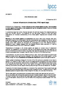


![AR5 Synthesis Report - Climate Change 2014 - IPCC [PDF]](https://m.moam.info/img/260x300/ar5-synthesis-report-climate-change-2014-ipcc-pdf_647dfa43098a9ef0458b461e.jpg)


