fluid with free boundaries have been receiving more ... moving boundaries, free surface) in which the mesh .... fixed), and for Subdomain 2 we impose free.
12th WSEAS Int. Conf. on APPLIED MATHEMATICS, Cairo, Egypt, December 29-31, 2007
31
Arbitrary Lagrangian-Eulerian method for coupled Navier-Stokes and convection-diffusion equations with moving boundaries LILIANA BRAESCU a and THOMAS F. GEORGE b a Department of Computer Science West University of Timisoara Blv. V. Parvan 4, Timisoara, 300223 ROMANIA b
Office of the Chancellor and Center for Nanoscience Departments of Chemistry & Biochemistry and Physics & Astronomy University of Missouri–St. Louis St. Louis, MO 63121 USA http://www.info.uvt.ro/~braescu/ Abstract: - Using the arbitrary Lagrangian-Eulerian method, an accurate description of the melt flow and impurity distribution in a time-dependent domain Ω(t), t ∈ [0, T], is performed. The procedure is developed for a crystal fiber grown from the melt by the edge-defined film-fed growth (EFG) technique, on the basis of the finite-element method using COMSOL Multiphysics software. For this, an EFG system without melt replenishment (the melt level in the crucible decreases in time) is considered. By coupling three application modes − incompressible Navier-Stokes, moving mesh arbitrary Lagrangian-Eulerian, and convection-diffusion − it is illustrated, in the time-dependent case, how the pull of the crystal, with a constant rate vin, generates the fluid flow, and it is shown how the resulting fluid flow and deformed geometry determine the impurity distribution in the melt and in the crystal. Key-Words: - Arbitrary Lagrangian-Eulerian method, Finite-element method, Free boundaries problems, Edge-defined film-fed growth technique, Single crystal fiber
1 Introduction Numerical simulations of viscous incompressible fluid with free boundaries have been receiving more attention over the past few decades. These types of problems arise frequently in several important industrial applications, such as melting and solidification, crystal growth, glass and metal forming processes, etc. A fundamentally important consideration in developing a computer code for simulating problems of these types is the choice of an appropriate kinematical description of the continuum, which determines the relationship between the deforming continuum and the finite grid or mesh of computing zones, and which provides an accurate resolution of material interfaces and mobile boundaries. Algorithms usually use two classical descriptions of motion: the Lagrangian description and the Eulerian description [1-2]. The Lagrangian is preferred for “contained fluids” in which there is only small motion or for solid mechanics where the displacements are relatively small, whereas the
Eulerian is preferred for any flow model (except moving boundaries, free surface) in which the mesh would be highly contorted if required to follow the motion. The main disadvantage of the Lagrangian algorithm is its inability to follow large distortions of the computational domain without recourse to frequent re-meshing operations. The disadvantages of the Eulerian algorithm are: (i) material interfaces lose their sharp definitions as the fluid moves through the mesh, and (ii) local regions of fine resolution are difficult to achieve. A hybrid approach which combines the best features of both the Lagrangian and Eulerian descriptions while minimizing their disadvantages is the arbitrary Lagrangian-Eulerian (ALE) technique [3-5]. This technique is associated with a moving imaginary mesh which follows the fluid domain. Denoting the velocity of the domain by w, in the Eulerian approach w is zero, and in the Lagrangian approach w is equal to the velocity of the fluid particles. In the ALE approach, w is equal to neither zero nor the velocity of the fluid particles, but varies
12th WSEAS Int. Conf. on APPLIED MATHEMATICS, Cairo, Egypt, December 29-31, 2007
smoothly and arbitrarily between both of them. This arbitrary mesh velocity keeps the movement of the meshes under control according to the physical problem, and it depends on the numerical simulation. More precisely, this method seems to be the Lagrangian description in zones and directions where “small” motion takes place, and the Eulerian description in zones and directions where it would be not be possible for the mesh to follow the motion of the fluid. In this paper, an accurate description of the melt flow and impurity distribution in a time-dependent domain Ω(t), t ∈ [0, T], on the basis of the finiteelement method, is performed using COMSOL Multiphysics software. Because the geometry (actually the mesh) changes shape, the ALE algorithm is involved. Thus, for determining the impurity distribution in the melt and in the crystal when the fluid domain changes in time, three application modes are coupled in the time-dependent case: incompressible Navier-Stokes (NS), moving mesh ALE, and convection-diffusion (CD). This coupling procedure is developed for a crystal fiber grown from the melt by edge-defined film-fed growth (EFG) technique without melt replenishment, and it demonstrates the ability of COMSOL to simulate flow and concentration evolutions with the help of the moving mesh. The mathematical model is formulated in two dimensions in a cylindrical-polar coordinate system attached to the center of the capillary channel (see Fig. 1). This is for an Al-doped Si fiber grown from the melt by the EFG method with a central capillary channel shaper (CCC) [6] and without replenishment.
32
viscosity, t is the time, and D is the impurity diffusion.
2 Mathematical description The fluid flow and the impurity distribution in the crucible, in the capillary channel and in the meniscus is described in a time-dependent domain Ω(t), t ∈ [0, T], by the incompressible Navier-Stokes and the conservative convection-diffusion equations, ⎧ ∂u T + ρl (u ⋅ ∇)u = ∇ ⋅ − pI + η ∇u + ∇u + F ⎪ρl ⎪ ∂t , (1) ⎨ ∇ ⋅u = 0 ⎪ ∂c ⎪ ∂t + ∇ ⋅ (−D∇c + cu) = 0 ⎩
[
(
( ) )]
for which axisymmetric solutions are searched in the cylindrical-polar coordinate system (rOz) (see Fig.1). In the system (1), u =(ur, uz) is the velocity vector, c is the impurity concentration, F =(0, - ρl ⋅ g ) is the volume force field due to the gravity, ρl is the melt density, p is the pressure, η is the dynamical
Fig. 1: Schematic diagram of the EFG system and boundary regions used in the numerical model.
12th WSEAS Int. Conf. on APPLIED MATHEMATICS, Cairo, Egypt, December 29-31, 2007
The evolution of Ω(t) = {(r(R, Z, t), z(R, Z, t))⏐(R,Z) ∈ Ω(0)} is described by the system of partial differential equations corresponding to the Laplace smoothing (Poisson equations): ⎧ ∂ 2 ⎛ ∂r ⎞ ∂ 2 ⎛ ∂r ⎞ ⎪⎪ ∂R 2 ⎜ ∂t ⎟ + ∂Z 2 ⎜ ∂t ⎟ = 0 ⎝ ⎠ ⎝ ⎠ . (2) ⎨ 2 2 ∂ ∂ ∂ ∂z ⎞ z ⎛ ⎞ ⎛ ⎪ ⎜ ⎟+ ⎜ ⎟=0 ⎪⎩ ∂R 2 ⎝ ∂t ⎠ ∂Z 2 ⎝ ∂t ⎠ Here R, Z represent the reference coordinates in the reference frame (ROZ), i.e., the fixed frame used for the description of Ω(t) and of the mesh velocity, as it is represented in Fig. 1(a-b). The solution (r(R, Z, t), z(R, Z, t)) satisfies the condition (r(R, Z, 0), z(R, Z, 0))=(R, Z). The coupled system (1-2) is considered in the two-dimensional domain Ω(t) with boundaries (Ω1) – (Ω12), and for solving it, the ALE technique is used. The moving mesh (ALE) application mode solves the system of partial differential equations (2) for the mesh displacement. This system smoothly deforms the mesh given by constraints on the boundaries. By the Laplace smoothing option (which has been chosen), the software introduces deformed mesh positions as degrees of freedom in the model. For solving the coupled system of PDE (1-2), boundary conditions on Ω1 to Ω12 are imposed, with the Oz-axis being considered as a line of symmetry for all field variables: (i) Flow (NS) conditions: On the melt/solid interface, the condition of outflow velocity is imposed,
i.e.,
u=
ρl ⋅v k , ρ s in
where
k
represents the unit vector of the Oz-axis. On the melt level in the crucible Ω9 and on the intern boundary Ω8, we set up the neutral condition,
( )
⎡ − pI + η ⎛⎜ ∇ u + ∇ u T ⎞⎟ ⎤ n = 0 , where n ⎢⎣ ⎝ ⎠ ⎥⎦
is the
normal vector. The other boundaries are set up by the non-slip condition u = 0 . (ii) Moving mesh (ALE) conditions: The domain Ω(t) is divided in two subdomains (labeled 1 and 2 − see Fig. 1(a-b)). For Subdomain 1, we impose no displacement (i.e., Subdomain 1 is fixed), and for Subdomain 2 we impose free displacement (is free to move). Hence, the mesh displacement takes place only in subdomain 2, and it is constrained by the boundary conditions on the surrounding boundaries Ω7, Ω8, Ω9 and Ω11. The displacement in Subdomain 2 is obtained by solving the system (2). The
33
boundary conditions involve variables from the NS application mode. To obtain convergence, it is important for the boundary conditions to be consistent. The usual point-wise constraints or ideal constraints for ALE cause unwanted modifications of the boundary condition for the other two application modes (NS and CD). For this reason, in the ALE application mode, we must use non-ideal weak constraints on the boundaries: - the mesh displacements in the r-direction and z-direction on Ω9 are dr = 0, dz = vn×t, where
R *2 ⋅ vin (according to [3-5] the vn = − 2 Rc − R02 mesh velocity should be equal to the fluid velocity); - the mesh displacement in the r-direction on Ω7UΩ11 is dr = 0; the mesh displacement dz in the z-direction is not specified, i.e., the mesh will follow the fluid movement; - the mesh displacements dr and dz in the rdirection and z-direction are not specified on Ω8 (the mesh follows the fluid flow). (iii) Concentration (CD) conditions: On the melt/solid interface, the flux condition is imposed, which expresses that impurities are rejected back into the melt according to v ∂c = − in (1− K 0 )c . On the inner boundary Ω8, D ∂n we set up the continuity condition (flux difference is zero), n ⋅ ( N1 − N 2 ) = 0, N i = − Di ∇ci + ci u i , where i = 1 for Subdomain 1 and i = 2 for Subdomain 2. The other boundaries are set up by the noimpurity flux condition, i.e., insulation:
∂c = n ⋅ ∇c = 0 . ∂n
Besides the above boundary conditions, we have to add the initial conditions: - for the fluid flow: u(t0) = 0, v(t0) = 0 in Subdomain 1 and u(t0) = 0, v(t0) = vn in Subdomain 2 (according to [3-5] the fluid velocity should be equal to the mesh velocity); - for the pressure: p(t0 ) = P0 = − ρ l ⋅ g ⋅ z in Subdomain 1 and p(t0) = 0 in Subdomain 2; - for the initial impurity distribution: c = C0 = c(t0 ) in both subdomains; - for the mesh displacement: r(t0)=R, z(t0)=Z. Details concerning the significance of these quantities and their values for the Al-doped Si rod are presented in Table 1 and Fig. 1(c).
12th WSEAS Int. Conf. on APPLIED MATHEMATICS, Cairo, Egypt, December 29-31, 2007
Table 1: Material parameters for silicon. Nomenclature c impurity concentration (mol/m3) C0 alloy concentration (mol/m3) D impurity diffusion (m2/s) Dl die length (m) g gravitational acceleration (m/s2) h meniscus height (m) K0 partition coefficient η dynamical viscosity (Kg/m×s) p pressure (Pa) R* crystal radius (m) Rcap capillary channel radius (m) Rc inner radius of the crucible (m) R0 die radius (m) ρl density of the melt (Kg/m3) ρs density of the crystal (Kg/m3) u velocity vector vin pulling rate (m/s) z coordinate in the pulling direction
Value
34
will be the one determined by the spatial coordinates r, z of the ALE frame in which the mesh is moving, i.e., (r, z) ∈ Ω(t).
0.01 5.3×10⁻⁸ 0.04 9.81 5×10⁻⁴ 0.002 7×10⁻⁴ 0 1.5×10⁻³ 1.5×10⁻³ 23×10-3 2×10⁻³ 2500 2300 10-6
3 Numerical results Numerical investigations are carried out for an Aldoped Si rod of radius R*=1.5 ×10⁻³ m, grown in terrestrial conditions with a pulling rate vin = 10-6 m/s. The boundaries presented in Fig.1 are determined from the particularities (characteristic elements) of the considered EFG growth system. Thus, a crucible with inner radius Rc = 23 ×10-3 m is considered in which a die of radius R0 = 2×10⁻³ m and length 40 ×10-3 m is introduced, such that 2/3 of the die is immersed in the melt. In the die, a capillary channel is manufactured with a radius Rcap= 1.5 ×10⁻³ m, through which the melt climbs up to the top of the die. A seed is placed in contact with the melt; due to the heat transfer, this seed melts, and a low meniscus with height h = 0.5×10⁻³ m is developed. These above values define the initial geometry Ω(0) in the fixed reference frame (ROZ), at t = 0. We then start the growth process of the Aldoped Si rod with a constant pulling rate vin. Because the EFG system is without melt replenishment (the melt level in the crucible decreases in time) and the crystal is pulled with a constant rate vin (at the boundary Ω3), a fluid flow in the crucible is induced. Hence, the melt height in the crucible decreases, i.e., the length of the boundaries Ω7, Ω11 decrease and the boundary Ω9 goes down. In this way, the initial geometry Ω(0) changes in time as Ω(t) = {(r(R, Z, t), z(R, Z, t))⏐(R,Z) ∈ Ω(0)} with respect to the reference frame (ROZ). The new reference frame
Fig. 2: Mesh deformation in the ALE application mode for vn = -4.65×10⁻⁸ m/s at three different moments of time, 0 < t1 < t2 < t3