Jan 19, 2006 - creasing need for computational power at an affordable cost. ..... need to be received from their hosting processor/partition. Again we would like ...
Architecture Aware Partitioning Algorithms
Technical Report
Department of Computer Science and Engineering University of Minnesota 4-192 EECS Building 200 Union Street SE Minneapolis, MN 55455-0159 USA
TR 06-001 Architecture Aware Partitioning Algorithms Irene Moulitsas and George Karypis
January 19, 2006
Architecture Aware Partitioning Algorithms
∗
Irene Moulitsas and George Karypis University of Minnesota, Department of Computer Science and Engineering and Digital Technology Center and Army HPC Research Center Minneapolis, MN 55455 {moulitsa, karypis}@cs.umn.edu
Abstract Existing partitioning algorithms provide limited support for load balancing simulations that are performed on heterogeneous parallel computing platforms. On such architectures, effective load balancing can only be achieved if the graph is distributed so that it properly takes into account the available resources (CPU speed, network bandwidth). With heterogeneous technologies becoming more popular, the need for suitable graph partitioning algorithms is critical. We developed such algorithms that can address the partitioning requirements of scientific computations, and can correctly model the architectural characteristics of emerging hardware platforms.
Keywords: graph partitioning, parallel algorithms, heterogeneous architectures, the Grid ∗
This work was supported in part by NSF EIA-9986042, ACI-0133464, ACI-0312828, and IIS-0431135; the Digital Technology Center at the University of Minnesota; and by the Army High Performance Computing Research Center (AHPCRC) under the auspices of the Department of the Army, Army Research Laboratory (ARL) under Cooperative Agreement number DAAD19-01-2-0014. The content of which does not necessarily reflect the position or the policy of the government, and no official endorsement should be inferred. Access to research and computing facilities was provided by the Digital Technology Center and the Minnesota Supercomputing Institute. Related papers are available via WWW at URL: http://www.cs.umn.edu/˜karypis.
1
1 Introduction Graph partitioning is a vital pre-processing step for many large-scale applications that are solved on parallel computing platforms. Over the years the graph partitioning problem has received a lot of attention [3, 12, 5, 1, 2, 7, 10, 11, 14, 15, 18, 19, 23, 20]. Despite the success of the existing algorithms, recent advances in science and technology demand that new issues be addressed in order for the partitioning algorithms to be effective. The Grid infrastructure [9, 4] seems to be a promising viable solution for satisfying the ever increasing need for computational power at an affordable cost. Metacomputing environments combine hosts from multiple administrative domains via transnational and world-wide networks into a single computational resource. Even though message passing is supported, with some implementation of MPI [8], there is no support for computational data partitioning and load balancing. Even on a smaller scale, clusters of PCs have become a popular alternative for running distributed applications. The cost effectiveness of adding new, and more powerful nodes to an existing cluster, and therefore increasing the cluster potential, is an appealing solution to a lot of institutions and researchers. We can clearly see that upcoming technologies have introduced a totally new class of architectural systems that are very heterogeneous in terms of computational power and network connectivity. Most of the graph partitioning algorithms mentioned above compute a data partitioning that is suitable for homogeneous environments only. Recently there has been some work on partitioning for heterogeneous architectures, namely PaGrid [16, 24], JOSTLE [22], MiniMax [21], and DRUM [6]. In [16] the multilevel paradigm is implemented, and a quadratic assignment problem is solved for the initial partitioning, followed by a refinement that aims at reducing the communication cost or the execution time of the application. Following a different direction, in [24] the initial partitioning is done arbitrarily, followed by a refinement that aims at reducing the sum of the execution times, over all the processors. JOSTLE does not take into account computational heterogeneity. It solves a quadratic assignment problem for the initial partitioning and minimizes some function of the total communication cost, without balancing communication costs between individual partitions though. MiniMax uses the multilevel approach, trying to minimize the execution time of the application. To account for communication, a modified function of the traditional edgecut metric is used. For the initial partitioning a graph growing algorithm is used. Finally, DRUM monitors the hardware resources and encapsulates all the information about a processor in a single scalar form. This scalar can be given as input to any of the traditional graph partitioning algorithms to guide load balancing. In the context of the widely used METIS [17] library we have developed graph partitioning algorithms for partitioning meshes/graphs onto heterogeneous architectures. Our algorithms allow full heterogeneity in both the computational and the communication resources. Unlike all the algorithms described in the previous paragraph, we do not use the notion of edgecut when estimating our communication. Instead, we use a more accurate model to describe the communication volume. We also avoid solving the expensive and unscalable quadratic assignment problem, and we do not enforce a dense processor-to-processor communication. 2
The remainder of this paper is organized as follows. Section 2.1 discusses the modeling of the computational/workload graph. In Section 2.2 we describe the heterogeneous architecture system model. In Section 3 we describe our proposed algorithms. Section 4 presents a set of experimental results and comparisons. Finally Section 5 provides some concluding remarks.
2 Problem Modeling The majority of multilevel graph partitioning problem formulations have primarily focused on edgecut based models and have tried to optimize edgecut based objectives. However, it is important to note that the edgecut metric is only an approximation of the total communication volume incurred by parallel processing [13]. This is because the actual communication volume may be lower than the edgecut. For example consider the case where two or more edges of a single vertex are connected to different vertices of another subdomain. In this case, the data associated with that vertex actually will be sent only once during the parallel application. However, with the edgecut model, this is not captured and all the edges account as multiple communication messages. In this case the correct measure of communication volume is the number of boundary vertices. However, this measure is harder to optimize than edgecut [13]. 2.1 Computational Graph Modeling The graph partitioning problem can be defined as follows: Given a graph G = (V, E), where V is the set of vertices, n = |V | is the number of vertices, and E is the set of edges in the graph, T S partition the vertices to p sets V1 , ..., Vp such that Vi Vj = ∅ for i 6= j and Vi = V , for i, j = 1, ..., p. This is called a p−way partitioning and is denoted by P . Every one of the subsets Vi , of the vertices of G, is called a partition or subdomain. P is represented by a partition vector of length n, such that for every vertex v ∈ V , P [v] is an integer between 1 and p, indicating the partition which a vertex v belongs to. The graph G is a weighted graph if every vertex v has two associated weights: w(v) and c(v). If no specific weights are provided, we can assume that all vertices, have uniform weights. Similarly to the traditional problem, the first vertex weight w is assigned depending on the amount of work/computations performed by a vertex. The second set of weights c is assigned to reflect the amount of data that needs to be sent between processors due to each vertex, i.e., communication. The Volume of a partitioning is the total communication volume required by the partition. For example, look at the two different partitionings presented in Figure 1 (a) and (b). Let’s assume vertex u and vertices u1 , u2 , u3 , u4 are assigned to partition P0 , while vertices v1 , v2 , v3 , v4 are assigned to partition P1 . For simplicity we have noted the communication weights of every vertex in the square brackets in the figure. So, we assume that c(u) = c(u 1 ) = . . . = c(u4 ) = c(v1 ) = . . . = c(v4 ) = 1. If the edgecut model were to be used, then each one of the cut edges would have an edge weight of 2, as each one of the incident vertices to the edge has communication size of 1. Both of the presented partitionings, in Figure 1(a) and Figure 1(b), would incur an edgecut of 8. However, in Figure 1(a) the actual communication volume is only 5. Indeed processor P0 will need to send a message of size 1 to P1 , and processor 1 will need to send four 3
P0
P0
P1 v1[1]
P1 u1[1]
2
u2[1]
2
u3[1]
2
2
v1[1]
v2[1]
v2[1]
2
u[1]
v3[1]
v3[1]
2 v4[1]
2
Edgecut = 4*2=8,
u4[1]
Volume = 1 + 4 = 5
Edgecut = 4*2=8,
Communication Volume = 5
v4[1]
2
Volume = 4 + 4 = 8
Communication Volume = 8
(a)
(b)
Figure 1: Comparison between the edgecut and volume models.
messages of size 1 to P0 . An estimate of the edgecut cannot distinguish between these two possible scenarios. On the other hand if the volume model is used, we will have an accurate estimate of the actual communication for both cases. 2.2 Architecture Graph Modeling Partitioning for a heterogeneous environment requires modeling the underlying computational architecture. The computational environment is modeled through a weighted undirected graph A = (P, L), that we call the Architecture Graph. P is the set of graph vertices, and they correspond to the processors in the system, P = {p1 , . . . , pp }, p = |P |. L is the set of edges in the graph, and they represent communication links between processors. The weights w ∗ (·) associated with the architecture graph vertices represent the processing cost per unit of computation. Each communication link l(pi , pj ) is associated with a graph edge weight e∗ (pi , pj ) that represents the communication cost per unit of communication between processors p i and pj . If two processors are not ”directly” connected, and the communication cost incurred between them needs to be computed, we can just sum the weights of the shortest path between them. For the algorithm presented in [22] it is shown that this linear path length (LPL) does not perform as well as the quadratic path length (QPL). Quadratic path length is the length where the squares of the individual path lengths are added up. The insight is that the LPL does not sufficiently penalize for cut edges across heavier links, i.e., links that suffer from slower communication capabilities. 1
4
8
12
16
20
24
28
32
Figure 2: 1D Array Processor Graph: Arch32_1.
In this section we present some typical architecture graphs that will also be used later for the evaluation of our algorithms. Figure 2 presents a one dimensional array. Even though such machines are not common in practice, the concept can be very useful with regards to machines that incur a high communication latency. Figure 3 is a two dimensional array. Figure 4 presents an 8– 4
1
2
3
4
8
7
6
5
9
10
11
12
16
15
14
13
17
18
19
20
24
23
22
21
25
26
27
28
32
31
30
29
Figure 3: 2D Array Processor Graph: Arch32_2.
node, 32–processor cluster. Each node has four tightly connected processors, and a fast interconnection network among its 4 processors. Communication between different nodes is slower, and we therefore use thicker lines to connect the nodes in the figure. Figure 5 shows a metacomputer that is made up from two supercomputers that each has 16 processors. Again the communication within the two compute nodes is faster than the one across the nodes. Finally, Figure 6 shows a typical grid architecture. The top and bottom part may each be physically located in the same geographical location and each is a metacomputer. These two metacomputers can then be combined to form a new metacomputer. The interconnection network between the two parts is slower than the one that is local for each one. For our model we assume that communication in either direction across a given link is the same, therefore e∗ (pi , pj ) = e∗ (pj , pi ), for i, j = 1, . . . , p. We also assume that e∗ (pi , pi ) = 0, as the cost for any given processor to retrieve information from itself is incorporated in its computational cost w∗ (pi ). For the case of the processor graph in Figure 7, that is a 1D array of 5 processors, if we assume that between neighboring processors the link weight is 1, then the communication cost, for a fully connected architecture graph will be:
0 1 2 3 4
1 0 1 2 3
2 1 0 1 2 5
3 2 1 0 1
4 3 2 1 0
11
10
8
7
12
9
14
13
5
4
15
18
16
6
17
3
19
1 32
2
31
22
29
21
25
30
20
28
23
24
26
27
Figure 4: Cluster of 8 compute nodes: Arch32_3.
Although the existing heterogeneous partitioning algorithms assume a complete weighted architecture graph, just as the one presented above for the 1D array, we find that this approach is not scalable and therefore avoid it. We provide more details in Section 3. 2.3 Metrics Definition Given the proposed models for the computational graph and the architecture graph, we now define several metrics that will be used in our partitioning algorithms. 2.3.1
Computational Cost
The first metric is the Computational Cost, i.e. the cost a processor p i will incur for processing a vertex v assigned to it by a given partitioning. This is given by CompCostvpi = w∗ (pi ) × w(v). To find the total time processor pi will need to perform computations, over all its assigned portion of vertices Vi of the computational graph: CompCostVpii = w∗ (pi ) ×
X
w(v)
v∈Vi
Again, the computational cost reflects the time needed by a certain processor to process the vertices assigned to it. 6
12
13
20
14
21
22
19
11
23
15
10
18
24
1
17
25
2
32
26
16
9 8 7
31
3 6
27
4
5
30
29
28
Figure 5: Metacomputer: Arch32_4. 2.3.2
Communication Cost
The second metric is the Communication Cost, i.e. the cost a processor p i will incur for communicating, sending and receiving, the necessary information in order to perform the parallel computation. As Figure 8 shows, each partition can distinguish between three types of vertices: 1. Interior (local) vertices, those being adjacent only with local vertices, 2. Local interface vertices, those being adjacent both with local and non–local vertices, and 3. External interface nodes, those vertices that belong to other partitions but are coupled with vertices that are assigned to the local partition. As a matter of fact, we do not need to worry about vertices that fall under category 1., as they do not account for any communication. On the other hand, vertices that belong to category 2. will need to be sent to the corresponding neighboring processors, and vertices belonging to category 3. will need to be received from their hosting processor/partition. Again we would like to emphasize the fact that we are talking about a vertex being sent to neighboring partitions, and not to neighboring vertices as the edgecut model would erroneously do. More complex data structures need to be maintained in order to achieve this, but thus we ensure the validity of the model. The cost that a processor pi will incur for communicating any information relevant to a vertex v assigned to it, is the cost to send any information plus the cost to receive any information: CommCostvpi =
X
e∗ (pi , P (w)) × c(v) +
P (w),w∈adj(v)
X
e∗ (pi , P (w)) × c(w),
w∈adj(v)
where adj(v) indicates the vertices adjacent to vertex v. To find the total time a processor p i will spend on performing communication, we sum over all its assigned portion of the vertices V i of the computational graph: CommCostVpii = 7
30
31
29
32 22
21
25
23
28
27
24
26
12
13
14
11
18 15 19
10 17
16 9
1
8
20
2 7
3 6
5
4
Figure 6: Metacomputer: Arch 32_5.
Figure 7: 1D Array Processor Graph.
X
v∈Vi
X
P (w),w∈adj(v)
e∗ (pi , P (w)) × c(v) +
X
v∈Vi
X
w∈adj(v)
e∗ (pi , P (w)) × c(w) .
In the above equation, please note that no communication links are double counted. For example look at Figure 9 and more specifically at vertex u2 . u2 will be sent to P1 as it is connected to v2 . Therefore it will not be sent again due to its connectivity with v 3 . Similarly vertex v1 will be received by processor P0 once for the connection with u1 . Therefore, it will not be received again due to its connection to vertex u2 . 2.3.3
Processor Elapse Time
For every processor pi , its elapse time (ElTime) is the time it spends on computations plus the time it spends on communications. Therefore, by using the above definitions, the elapse time of processor pi is given by: ElapseT imeVpii = CompCostVpii + CommCostVpii
8
P3
Local Interface nodes
External Interface nodes
P0
P1 P2
Figure 8: A view of a partition’s vertices. 2.3.4
Processor Overall Elapse Time
By summing up the elapse times of all individual processors, we have an estimate of the overall time (SumElTime) that all processors will be occupied. T otalElapseT ime =
X
ElapseT imeVpii
pi
2.3.5
Application Elapse Time
The actual run time of the parallel application (MaxElTime) will be determined by that processor that needs the most time to complete. Therefore, no matter how good the quality of a partitioning is, its overall performance is driven by its ”worst” partition. ElapseT ime = maxpi {ElapseT imeVpii }
3 Graph Partition Algorithm There are a variety of approaches that can be applied here. They are all based on extending the multilevel paradigm of METIS [17] to account for the heterogeneity of the architecture infrastructure. In particular, the classical coarsening/initial partitioning/refinement stages are augmented so that they take into account the different communication costs and computational capabilities. We try to solve the problem by decoupling the computational from the communication requirements. During the initial partitioning phase we compute a partitioning that balances the overall computation. The multilevel paradigm is used and during the last phase, which is the refinement phase, we balance the partitions based on the computational capabilitites of the undelying architecture algorithm. However, communication is still not addressed. After the multilevel partitioning algorithm has 9
P0
P1 v1[1] u1[1] u2[1]
v2[1]
u3[1]
v3[1]
Communication Volume = 4 Figure 9: Communication Volume.
completed, we augment the algorithm with an additional refinement step. During this new refinement phase a different metric is optimized so that the communication volume is minimized. Therefore at this stage, vertices are moved among partitions and the objective function taken into consideration is the volume of communication incurred. A general overview of the approach is shown in Figure 10.
Figure 10: Our two-phase approach.
The drawback of the above algorithm is that it is not easily scalable. Indeed as we move to a larger number of partitions the potential refinement moves between processors can get very costly to determine. A variation of this algorithm can be implemented. While refinement moves are performed among partitions, these moves are restricted so that no new communication links are created, between partitions/processors that were not connected through the initial partition. Therefore we also minimize the communications overhead. In this fashion we have kept a sparse form of the communication matrix and this does not limit our algorithms from scaling to larger number of processors. 10
A different approach we are considering is changing the objective function of the refinement stage. Given a partitioning of the computational graph we can estimate the execution time of the parallel application, see Section 2.3. Therefore, it would make more sense to perform vertex refinement moves so that the maximum time is minimized (and therefore the overall time of the application), and individual processor elapse times are balanced. Again a variation of this algorithm can be implemented so that the moves during the refinement phase, are considered and performed in a sparse fashion, while the objective function of the application elapse time is used.
4 Experimental Results We evaluated the performance of our algorithms using a wide variety of graphs and architecture topologies. The description and characteristics of the computation graphs are presented in Table 1. The size of these graphs ranged from 14K to 1.1M vertices. 1
Name 144
# Vertices 144, 649
# Edges 1, 074, 393
2
auto
448, 695
3, 314, 611
3
brack2
62, 631
366, 559
4 5
cylinder93 f16
45, 594 1, 124, 648
1, 786, 725 7, 625, 318
6
f22
428, 748
3, 055, 361
7
finan512
74, 752
261, 120
8
inpro1
46, 949
1, 117, 809
9
m6n
94, 493
666, 569
Description Graph corresponding to a 3D FEM mesh of a parafoil Graph corresponding to a 3D FEM mesh of GM’s Saturn Graph corresponding to a 3D FEM mesh of a bracket Graph of a 3D stiffness matrix Graph corresponding to a 3D FEM mesh of an F16 wing Graph corresponding to a 3D FEM mesh of an F22 wing Graph of a stochastic programming matrix for financial portofolio optimization Graph corresponding to a 3D stiffness matrix Graph corresponding to a 3D FEM mesh of an M6 wing
Table 1: Characteristics of the test data sets.
The architecture graphs we used were presented in Section 2.2. In particular, we used architectures Arch32 1 as in Figure 2, Arch32 2 as in Figure 3, Arch32 3 as in Figure 4, and finally Arch32 5 as in Figure 6. In order to explore full heterogeneity of our architecture model, the weights on the computational nodes, as well as the weights on the communication links were arbitrary. In the rest of this section we compare the results for all of our four proposed algorithms. Labels VolNS, VolS, ElTNS, ElTS, correspond to our partitioning algorithms as described in Section 3. Wherever used, Initial corresponds to the graph partitioning algorithm that only takes into consideration the computational capabilities of the underlying architecture. We use these names so that 11
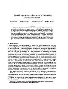
the following figures will be easily readable. 4.1 Quality of the Results For each one of our computation graphs and architectures mentioned above we have assessed five different qualities. These are shown respectively in graphs (a), (b), (c), (d), and (e) of Figure 11, Figure 12, Figure 13, and Figure 14 and discussed below. 4.1.1
Elapse Time Balance Assessment
We define the elapse time imbalance of a p-way partitioning P as ElapseT ime(Im)balance(P ) =
maxp {ElapseT imeVpii } ElapseT ime , = P i T otalElapseT ime/p ( pi ElapseT imeVpii )/p
which is the ratio of the time the application will need to complete over the average run time of all involved processors. Looking at the results in part (a) of the figures we can see that we are able to improve the balance of the resulting partitionings by performing a refinement strategy after the initial partition is computed that only takes into account the computational capabilities. 4.1.2
Elapse Time Assessment
As we have discussed earlier the overall quality of a partitioning depends on the quality of the worst partition, i.e. the partition/processor that will need the most time to complete. Therefore, for each one of our experiments we computed the estimated Application Elapse Time, as defined in Section 2.3.5. This time varies a lot, depending on the size and connectivity of the computational graph. Thus, in parts (b) of our figures we present the relative time compared to that of our Initial partitioning. From these figures we can easily see that our algorithms produce partitions of higher quality. Since the ratio is always smaller than one, the applications that use these new partitioning algorithms will run faster. We can also see that our algorithms that perform refinement using the elapse time objective function perform better than the ones that use the communication volume objective function. 4.1.3
Processor Overall Elapse Time Assessment
One more measure that we have evaluated is the processor overall elapse time, as it was defined in Section 2.3.4. Again we present the relative ratio between the refinement algorithms and our Initial partitioning algorithm. As we see in figures (c), of all the 36 experiments presented for each one of our algorithms, only very few, produced partitions of higher processor overall elapse time, i.e. very few times did we cross above the 1 ratio line. However, even in these few cases, the reason we allowed this to occur, was in order to minimize the application elapse time only. Indeed, if we look at Figure 11(c), we see that for our sixth dataset, the third algorithm produced slightly higher processor overall times. At the same time though, the same algorithm was able to reduce the application time by 40% as we see in Figure 11(b). 12
4.1.4
Edgecut .vs. Volume Assessment
In figures (d) and (e) we present the relative partition edgecut and volume compared to the one of the Initial algorithm. As we can see in figures (d), for most of our experiments the edgecut of our partitions is higher compared to the initial one. On the other hand though we can see that eventhough the edgecut is higher, the actual communication volume, as shown in figures (e), is lower. This is a proof towards the argument that eventhough the edgecut gives an indication of the communication volume, it is by no means an accurate measure of it. Indeed, by looking at figures (d) we would have been misled as to say the our algorithms would have higher communication needs. But when the actual communication volumes are estimated, we see in (e) that the actual communication is decreased.
13
Elapse Time Imbalnce Arch 32_1 Initial
Vol NS
Vol S
ElT NS
ElT S
9 8 7 6 5 4 3 2 1 0 1
2
3
4
5
6
7
8
9
Data Sets
(a) Sum El time New .vs. Initial, Arch 32_1
Max El Time New .vs. Initial, Arch 32_1 Vol NS
Vol S
ElT NS
ElT S
Vol NS
1,2
1,2
1
1
0,8
0,8
0,6
0,6
0,4
0,4
0,2
0,2
Vol S
ElT NS
ElT S
0
0 1
2
3
4
5 6 Data Sets
7
8
1
9
2
3
4
5
(b) Vol S
7
8
9
8
9
(c) Volume New .vs. Initial, Arch 32_1
Edgecut New .vs. Initial, Arch 32_1 Vol NS
6
Data Sets
ElT NS
Vol NS
ElT S
1,6
1,2
1,4
1
Vol S
ElT NS
ElT S
1,2
0,8
1 0,8
0,6
0,6
0,4
0,4
0,2
0,2
0
0 1
2
3
4
5 6 Data Sets
7
8
1
9
2
3
4
5 Data Sets
(d)
(e)
Figure 11: Characteristics of the induced 32-way partitioning for Arch32_1.
14
6
7
Elapse Time Imbalance Arch 32_2 Initial
Vol NS
Vol S
ElT NS
ElT S
4 3,5 3 2,5 2 1,5 1 0,5 0 1
2
3
4
5
6
7
8
9
Data Sets
(a) Sum El Time New .vs. Initial, Arch 32_2
Max El Time New .vs. Initial, Arch 32_2
Vol NS
Vol NS
Vol S
ElT NS
ElT S
Vol S
ElT NS
ElT S
1,2
1,2 1
1 0,8
0,8 0,6
0,6 0,4
0,4
0,2
0,2
0
0
1
2
3
4
5 6 Data Sets
7
8
9
1
2
3
4
(b) Vol S
6
7
8
9
8
9
(c) Volume New .vs. Initial, Arch 32_2
Edgecut New .vs. initial, Arch 32_2 Vol NS
5
Data Sets
ElT NS
ElT S
Vol NS
1,6
Vol S
ElT NS
ElT S
1,2
1,4 1
1,2 1
0,8
0,8
0,6
0,6 0,4
0,4 0,2
0,2 0
0
1
2
3
4
5
Data Sets
6
7
8
9
1
(d)
2
3
4
5
Data Sets
(e)
Figure 12: Characteristics of the induced 32-way partitioning for Arch32_2.
15
6
7
Elapse Time Imbalance Arch 32_3 Initial
Vol NS
Vol S
ElT NS
ElT S
3,5 3 2,5 2 1,5 1 0,5 0 1
2
3
4
5
6
7
8
9
Data Sets
(a) Sum El Time New .vs. Initial, Arch 32_3
Max El Time New .vs. Initial, Arch 32_3
Vol NS
Vol S
ElT NS
ElT S
Vol NS
1,2
Vol S
ElT NS
4
5
ElT S
1,2
1
1
0,8
0,8
0,6
0,6
0,4
0,4
0,2
0,2
0
0
1
2
3
4
5
Data Sets
6
7
8
9
1
2
3
(b) Vol S
6
7
8
9
8
9
(c)
Edgecut New .vs. Initial, Arch 32_3 Vol NS
Data Sets
ElT NS
Volume New .vs. Initial, Arch 32_3 Vol NS
ElT S
1,4
1,2
1,2
1
Vol S
ElT NS
ElT S
1
0,8 0,8
0,6 0,6
0,4
0,4
0,2
0,2 0
0 1
2
3
4
5
6
7
8
9
1
Data Sets
2
3
4
5
Data Sets
(d)
(e)
Figure 13: Characteristics of the induced 32-way partitioning for Arch32_3.
16
6
7
Elapse Time Imbalance Arch 32_5 initial
Vol NS
3
4
Vol S
ElT NS
ElT S
8 7 6 5 4 3 2 1 0 1
2
5 Data Sets
6
7
8
9
(a) Sum El Time New .vs. Initial, Arch 32_5
Max El Time New .vs. Initial, Arch 32_5 Vol NS
Vol S
ElT NS
Vol NS
ElT S
1,2
1,2
1
1
0,8
0,8
0,6
0,6
0,4
0,4
0,2
0,2
Vol S
ElT NS
ElT S
0
0 1
2
3
4
5 6 Data Sets
7
8
1
9
2
3
4
(b)
7
8
9
8
9
(c)
Edgecut New .vs. Initial, Arch 32_5
Vol NS
5 6 Data Sets
Vol S
ElT NS
Volune New .vs. Initial, Arch 32_5
ElT S
Vol NS
1,4
Vol S
ElT NS
ElT S
1,2
1,2
1
1
0,8 0,8
0,6 0,6
0,4 0,4
0,2
0,2
0
0 1
2
3
4
5
Data Sets
6
7
8
1
9
2
3
4
5
Data Sets
(d)
(e)
Figure 14: Characteristics of the induced 32-way partitioning for Arch32_5.
17
6
7
4.2 Comparison between sparse and non-sparse algorithms In this section we are showing the qualitative differences between the sparse and the non-sparse refinement approaches. As noted earlier, one of the main contributions of this work is that it also proposes sparse algorithms that are more scalable compared to the non-sparse refinement ones. Of course there lies a question regarding how much we have sacrificed in quality in order to achieve this scalability. In Figure 15 we want to compare the sparse volume refinement algorithm with its non-sparse counterpart, and the sparse elapse time refinement algorithm with the non-sparse one. To achieve this comparison we have taken the ratio of the application elapse times of the sparse algorithms, over the application elapse times of the non-sparse ones. We have a total of 72 comparisons. We can see that in only 5 of the cases, did the sparse scalable algorithms produce worse results. In the other 67 cases, the qualities were comparable, and therefore we did not see any degradation. Max El Time Sparse .vs. Non-sparse Arch 32_2
Max El Time Sparse .vs. Non-sparse Arch 32_1
Vol
Vol
ElT
ElT 1,6
1,4
1,4 1,2
1,2 1
1 0,8
0,8 0,6
0,6
0,4
0,4
0,2
0,2
0
0 1
2
3
4
5
6
7
8
9
1
2
3
4
Data Sets
(a)
5 Data Sets
6
7
8
9
(b) Max El Time Sparse .vs. Non-sparse Arch 32_5
Max El Time Sparse .vs. Non-sparse Arch 32_3 Vol
Vol
ElT
ElT
1,8
1,2
1,6
1 1,4
0,8
1,2 1
0,6
0,8
0,4
0,6
0,2
0,4 0,2
0 1
2
3
4
5
6
7
8
0
9
1
Data Sets
2
3
4
5
Data Sets
(c)
(d)
Figure 15: Comparison of the sparse and non sparse approaches.
18
6
7
8
9
5 Conclusions The field of heterogeneous graph partitioning is a very new field and there is a lot of room for improvement. However the approaches described above represent a scalable solution that merits further investigation and development. We were able to produce partitions of high quality that can correctly model architecture characteristics and address the requirements of upcoming technologies.
References [1] Stephen T. Barnard. Pmrsb: Parallel multilevel recursive spectral bisection. In Supercomputing 1995, 1995. [2] Stephen T. Barnard and Horst Simon. A parallel implementation of multilevel recursive spectral bisection for application to adaptive unstructured meshes. In Proceedings of the seventh SIAM conference on Parallel Processing for Scientific Computing, pages 627–632, 1995. [3] T. Bui and C. Jones. A heuristic for reducing fill in sparse matrix factorization. In 6th SIAM Conf. Parallel Processing for Scientific Computing, pages 445–452, 1993. [4] Steve J. Chapin, Dimitrios Katramatos, John Karpovich, and Andrew S. Grimshaw. The Legion resource management system. In Dror G. Feitelson and Larry Rudolph, editors, Job Scheduling Strategies for Parallel Processing, pages 162–178. Springer Verlag, 1999. [5] Pedro Diniz, Steve Plimpton, Bruce Hendrickson, and Robert Leland. Parallel algorithms for dynamically partitioning unstructured grids. In Proceedings of the seventh SIAM conference on Parallel Processing for Scientific Computing, pages 615–620, 1995. [6] Jamal Faik, Luis G. Gervasio, Joseph E. Flaherty, Jin Chang, James D. Teresco, Erik G. Boman, and Karen D. Devine. A model for resource-aware load balancing on heterogeneous clusters. Technical Report CS-03-03, Williams College Department of Computer Science, 2003. Submitted to HCW, IPDPS ’04. [7] C. M. Fiduccia and R. M. Mattheyses. A linear time heuristic for improving network partitions. In In Proc. 19th IEEE Design Automation Conference, pages 175–181, 1982. [8] Message Passing Interface Forum. MPI: A message-passing interface standard. Technical Report UT-CS-94-230, 1994. [9] I. Foster and C. Kesselman. Globus: A metacomputing infrastructure toolkit. The International Journal of Supercomputer Applications and High Performance Computing, 11(2):115–128, Summer 1997. [10] John R. Gilbert, Gary L. Miller, and Shang-Hua Teng. Geometric mesh partitioning: Implementation and experiments. In Proceedings of International Parallel Processing Symposium, 1995. [11] Todd Goehring and Yousef Saad. Heuristic algorithms for automatic graph partitioning. Technical report, Department of Computer Science, University of Minnesota, Minneapolis, 1994. [12] M. T. Heath and Padma Raghavan. A Cartesian parallel nested dissection algorithm. SIAM Journal of Matrix Analysis and Applications, 16(1):235–253, 1995.
19
[13] Bruce Hendrickson. Graph partitioning and parallel solvers: Has the emperor no clothes? (extended abstract). In Workshop on Parallel Algorithms for Irregularly Structured Problems, pages 218–225, 1998. [14] Bruce Hendrickson and Robert Leland. An improved spectral graph partitioning algorithm for mapping parallel computations. Technical Report SAND92-1460, Sandia National Laboratories, 1992. [15] Bruce Hendrickson and Robert Leland. A multilevel algorithm for partitioning graphs. Technical Report SAND93-1301, Sandia National Laboratories, 1993. [16] Sili Huang, Eric E. Aubanel, and Virendrakumar C. Bhavsar. Mesh partitioners for computational grids: A comparison. In Vipin Kumar, Marina L. Gavrilova, Chih Jeng Kenneth Tan, and Pierre L’Ecuyer, editors, ICCSA (3), volume 2669 of Lecture Notes in Computer Science, pages 60–68. Springer, 2003. [17] George Karypis and Vipin Kumar. METIS 4.0: Unstructured graph partitioning and sparse matrix ordering system. Technical report, Department of Computer Science, University of Minnesota, 1998. Available on the WWW at URL http://www.cs.umn.edu/˜metis. [18] George Karypis and Vipin Kumar. Multilevel k-way partitioning scheme for irregular graphs. Journal of Parallel and Distributed Computing, 48(1):96–129, 1998. Also available on WWW at URL http://www.cs.umn.edu/˜karypis. [19] George Karypis and Vipin Kumar. A fast and highly quality multilevel scheme for partitioning irregular graphs. SIAM Journal on Scientific Computing, 20(1), 1999. Also available on WWW at URL http://www.cs.umn.edu/˜karypis. A short version appears in Intl. Conf. on Parallel Processing 1995. [20] Kirk Schloegel, George Karypis, and Vipin Kumar. Graph partitioning for high performance scientific simulations. In J. Dongarra et al., editor, CRPC Parallel Computing Handbook. Morgan Kaufmann, 2000. [21] Rupak Biswas Shailendra Kumar, Sajal K. Das. Graph partitioning for parallel applications in heterogeneous grid environments. In Proceedings of the 2002 International Parallel and Distributed Processing Symposium, 2002. [22] C. Walshaw and M. Cross. Multilevel Mesh Partitioning for Heterogeneous Communication Networks. Future Generation Comput. Syst., 17(5):601–623, 2001. (originally published as Univ. Greenwich Tech. Rep. 00/IM/57). [23] Chris Walshaw and Mark Cross. Parallel optimisation algorithms for multilevel mesh partitioning. Parallel Computing, 26(12):1635–1660, 2000. [24] Renaud Wanschoor and Eric Aubanel. Partitioning and mapping of mesh-based applications onto computational grids. In GRID ’04: Proceedings of the Fifth IEEE/ACM International Workshop on Grid Computing (GRID’04), pages 156–162, Washington, DC, USA, 2004. IEEE Computer Society.
20