Multilevel Algorithms for Multi-Constraint Graph Partitioning

Multilevel Algorithms for Multi-Constraint Graph Partitioning∗ George Karypis and Vipin Kumar University of Minnesota, Department of Computer Science / Army HPC Research Center Minneapolis, MN 55455 Technical Report # 98-019 {karypis, kumar}@cs.umn.edu

Last updated on May 5, 1998 at 5:00pm

Abstract Traditional graph partitioning algorithms compute a k-way partitioning of a graph such that the number of edges that are cut by the partitioning is minimized and each partition has an equal number of vertices. The task of minimizing the edge-cut can be considered as the objective and the requirement that the partitions will be of the same size can be considered as the constraint. In this paper we extend the partitioning problem by incorporating an arbitrary number of balancing constraints. In our formulation, a vector of weights is assigned to each vertex, and the goal is to produce a k-way partitioning such that the partitioning satisfies a balancing constraint associated with each weight, while attempting to minimize the edge-cut. Applications of this multi-constraint graph partitioning problem include parallel solution of multi-physics and multi-phase computations, that underly many existing and emerging large-scale scientific simulations. We present new multi-constraint graph partitioning algorithms that are based on the multilevel graph partitioning paradigm. Our work focuses on developing new types of heuristics for coarsening, initial partitioning, and refinement that are capable of successfully handling multiple constraints. We experimentally evaluate the effectiveness of our multi-constraint partitioners on a a variety of synthetically generated problems.

∗ This work was supported by NSF CCR-9423082 and by Army Research Office contract DA/DAAH04-95-1-0538, and by Army High Performance Computing Research Center under the auspices of the Department of the Army, Army Research Laboratory cooperative agreement number DAAH04-95-2-0003/contract number DAAH04-95-C-0008, the content of which does not necessarily reflect the position or the policy of the government, and no official endorsement should be inferred. Access to computing facilities was provided by AHPCRC, Minnesota Supercomputer Institute, Cray Research Inc, and by the Pittsburgh Supercomputing Center. Related papers are available via WWW at URL: http://www.cs.umn.edu/˜karypis

1

1 Introduction The traditional graph partitioning problem focuses on computing a k-way partition of a graph such that the edge-cut is minimized and each partition has an equal number of vertices (or in the case of weighted graphs, the sum of the vertexweights in each partition are the same). The task of minimizing the edge-cut can be considered as the objective and the requirement that the partitions will be of the same size can be considered as the constraint. This single-objective single-constraint graph partitioning problem is widely used for static distribution of the mesh in parallel scientific simulations. Unfortunately, this single-objective single-constraint graph partitioning problem is not sufficient to model the underlying computational requirements of many large-scale scientific simulations. For example, in multi-phase mesh-based computations, single constraint is not sufficient to effectively balance the overall computations. Multi-phase computations consist of m distinct computational phases, each separated by an explicit synchronization step. In general, the amount of computations performed for each element of the mesh is different for different phases. In order to effectively solve such multi-phase computations in parallel, we must partition the mesh such that the computation in each phase is balanced, and the amount of interaction among the different processors in each phase is minimized. Note that the traditional single-constraint graph partitioning model is not effective in such computations. For example, if we assign to each node a weight that corresponds to the total amount of computations performed by all phases, we will get a partitioning that is not necessarily balanced during each computational phase (due to the explicit synchronization phases). An alternate solution to this problem is to obtain a different partitioning of the graph for each phase. This will balance the work and minimize interactions within each phase. However, transferring data among the different phases may incur high communication overhead, severely decreasing the overall performance of the computations. Ideally, we would like to treat the balancing of computations performed in each phase as separate constraints. Now the objective is to obtain a partitioning such that the communication is minimized subject to the constraints that the computations performed within each phase is balanced. As another example, consider the multi-physics simulation in which the amount of computation as well as the memory requirements are not uniform across the mesh. Existing single-constraint graph partitioning algorithms allow us to easily partition the mesh among the processors such that either the amount of computations is balanced or the amount of memory required by each partition is balanced; however, they do not allow to compute a partitioning that simultaneously balances both of these quantities. Our inability to compute such partitioning can either lead to significant computational imbalances, limiting the overall efficiency, or significant memory imbalances, limiting the size of the problems that we can solve using parallel computers. In many emerging applications there is also a need to produce partitionings that try to achieve multiple objectives. For example, a number of preconditioners have been developed that are focused on the subdomains assigned to each processor and ignore any intra-subdomain interactions (e.g., block diagonal preconditioners and local ILU preconditioners). In these preconditioners, a block diagonal matrix is constructed by ignoring any intra-domain interactions, a preconditioner of each block is constructed independently, and they are used to precondition the global linear system. The use of a graph partitioning algorithm to obtain the initial domain decomposition ensures that the number of non-zeros that are ignored in the preconditioning matrix is relatively small. However, existing graph models do not allow us to control both the number as well as the magnitude of these ignored non-zeros. Ideally, we would like to obtain a decomposition such that not only the number of intra-domain interactions is minimized (reducing the communication overhead) but also the numerical magnitude of these interactions is minimized (potentially leading to a better preconditioner). The key characteristic of these problems is that they require the partitioning algorithm to handle an arbitrary number of balancing constraints as well as an arbitrary number of minimization (or maximization) objectives. In this paper we focus on developing graph partitioning algorithms for effectively computing a k-way partitioning of a graph in the presence of an arbitrary number of balancing constraints. The problem of computing a partitioning when multiple objectives are present is discussed in [12]. We first present a generalized problem in which a vector of weights is assigned to each vertex. The goal is to produce a k-way partitioning such that the partitioning satisfies a balancing constraint associated with each weight,

2

while attempting to minimize the edge-cut (i.e., the objective function). We refer to it as a multi-constraint graph partitioning problem. This multi-constraint framework can be easily used to balance multi-phase computations, and balance memory and computational requirements. In the case of multi-phase computations, we can use as many balancing constraints as the number of phases. Balancing both computational as well as memory requirements can be achieved by using two constraints, one for the computational requirements and the other for the memory requirements. We present new multi-constraint graph partitioning algorithms that are based on the multilevel graph partitioning paradigm. Our work focuses on developing new types of heuristics for coarsening, initial partitioning, and refinement that are capable of successfully handling multiple constraints. We experimentally evaluate the effectiveness of our multi-constraint partitioners on a a variety of synthetically generated problems. Our experimental results show that our algorithms are able to effectively partition graphs with up to five different balancing constraints. Comparing the quality of these multi-constraint partitionings to those of the (much easier) single-constraint partitionings, we see that our algorithms lead to only a moderate increase in the number of edges that are cut by the partitioning. The rest of this paper is organized as follows. Section 2 introduces the multi-constraint graph partitioning problem and presents two formulations; the horizontal and the vertical formulation. Section 3 presents a theoretical analysis which shows that (a) problems for which a high-quality single-weight partitioning algorithm exists it can be used to compute a multi-constraint partitioning that has certain quality and balance guarantees; (b) there are algorithms that can compute highly-balanced partitionings for certain classes of multi-constraint problems. Section 4 describes the multilevel partitioning paradigm. Section 5 describes the multi-constraint formulation of the multilevel recursive bisection algorithm. Section 6 describes the multi-constraint formulation of the multilevel k-way partitioning algorithm. Section 7 presents an experimental evaluation of the multilevel multi-constraint algorithms. Finally, Section 8 presents some concluding remarks.

2 Problem Definition Consider a graph G = (V, E), such that each vertex v ∈ V has a weight vector wv of size m associated with it, and each edge e ∈ E has a scalar weight we . We place no restrictions on the weights of the edges but we will P assume, without loss of generality, that the weight vectors of the vertices satisfy the property that ∀v∈V wiv = 1.0 P for i = 1, 2, . . . , m. If the vertex weights do not satisfy the above property, we can divide each wiv by ∀v∈V wiv to ensure that the property is satisfied. Note that this normalization does not in any way limit our modeling ability. Let P be the partitioning vector of size |V |, such that for each vertex v, P[v] stores the partition number that v belongs to. For any such k-way partitioning vector, the load imbalance li with respect to the i th weight of the k-way partitioning is defined as follows: ! X li = k max wiv (1) j

∀v:P[v]= j

P If the i th weight is perfectly balanced in the k-way partitioning, then ∀v:P[v]= j wiv for all j is 1/k, and li = 1. A load imbalance of li = x indicates that a computation of size W performed on k processors during the i th phase takes x W/k time instead of W/ p time needed in the case of perfect load balance, under the assumption of zero communication overhead. A load imbalance of 1 + α indicates that the partitioning is load imbalanced by α%. We now define two distinct formulations of the multi-constraint graph partitioning problem: Horizontal Multi-constraint Partitioning Problem Find a k-way partitioning P of G such that the sum of the weights of the edges that are cut by the partitioning is minimized subject to the constraint ∀i, li ≤ ci . (2) Where c is a vector of size m such that ∀i, ci ≥ 1.0. Vertical Multi-constraint Partitioning Problem Find a k-way partitioning P of G such that the sum of the weights of the edges that are cut by the partitioning

3

is minimized subject to the constraint

m X

ri li ≤ c.

(3)

i=1

Where c is a scalar such that c ≥ 1.0, and r is a vector of size m such that ∀i, ri ≤ 1.0, and

P

i ri

= 1.0.

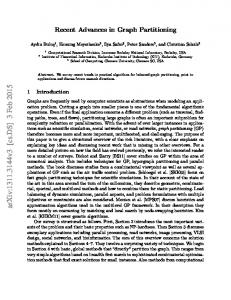
The horizontal multi-constraint partitioning problem tries to find a k-way partitioning such that each weight i is individually balanced within the tolerance specified by the i th entry of vector c. For example, if m = 2, (i.e., we have two weights), then the vector c = (1.05, 1.5) indicates that we are looking for a partitioning such that the load imbalance with respect to the first weight will be less than or equal to 5%, and that the load imbalance with respect to the second weight will be less than or equal to 50%. The horizontal formulation of the multi-constraint partitioning problem can be used, for example, to compute a partitioning that balances both computational and memory requirements. In particular, the ability of the model to handle a different tolerance for each individual weight is particularly useful in such a situation. In this example, the object is to get as tight a balance as possible with respect to the computational load (i.e., the corresponding entry of c is close to 1.0), whereas a somewhat higher load imbalance with respect to memory is allowable if it improves the quality of the partitioning (i.e., reduces the edge-cut). The horizontal formulation can also be used to balance multiphase-computations by setting the tolerance for each of the weights to the desired upper bound on load imbalance. For example, if we want to achieve a maximum of 5% load imbalance, we can set ci = 1.05 for i = 1, 2, . . . , m. However, this formulation limits our ability to find good partitionings. For example, consider the case of a three phase computation such that the overall work performed in each phase is the same. For this computation, a partitioning with a load imbalance vector of (1.02, 1.04, 1.09) will still satisfy the global load imbalance of 1.05, and should be preferred if it leads to a smaller edge-cut over a partitioning with a load imbalance of (1.05, 1.05, 1.05). This limitation becomes even more serious when the amount of computation performed in each phase is significantly different. For example, consider the multiphase computation with three phases as shown in Figure 1. For the first two phases, computation is performed over large portions of the domain whereas in the third phase, only a small region of the domain is involved in the computations. Further assume that in each of the three phases, the amount of computation performed for each element is the same. A partitioning algorithm that tries to balance each weight separately, will be forced to compute a partitioning of the region that is active in the third phase. However, since we know that the first two phases perform significantly more computations than the third phase, we can relax the balancing tolerance of the third phase by slightly tightening the tolerance of the first two phases. For instance, if each of the first two phases accounts for 45% of the computation, and the third phase accounts for the remaining 10%, then we can ensure an overall load imbalance of 5% by setting the tolerance for the first two phases to be 1.03, and the tolerance of the third phase to be 1.23. Phase I

Phase II

Phase III

Figure 1: Equally balancing the computations of each phase will lead to the active part of the third phase (shaded region) to be split into k parts. In general, if ri is the fraction of the overall computation performed in phase i and li is the load imbalance for P phase i , then the overall load imbalance of performing this multi-phase computation is m i=1 ri li . This is exactly what the vertical formulation of the multi-constraint graph partitioning tries to achieve. This formulation takes as input a vector r, that provides the relative weighting of each one of the constraints, and it computes a partitioning that minimizes the cut while the global load imbalance is constrained by c. In general, the vertical formulation is useful when the different constraints are of the same nature (for example, they all represent computation time), as is the case 4

of multiphase computations. Note that this formulation allows (and encourages) the use of different upper bound on load imbalance for each phase. If ci is the maximum load imbalance tolerated for phase i , then the overall load imbalance for performing P Pm this multiphase computation is bounded by m i=1 ri ci . A vector c is acceptable if i=1 ri ci ≤ c. Given a vector r, many different values for c are acceptable. For example, for a three-phase problem, if r = (1/3, 1/3, 1/3) and desired load imbalance is c = 1.05, then c1 = (1.05, 1.05, 1.05) and c2 = (1.02, 1.04, 1.09) are both acceptable. Relative merit of different possible values of c depends upon many factors including the actual distribution of computations across different phases. Hence, it is not desirable to pre-assign the values of c. It appears better to let the partitioning algorithm select these relaxed bounds on the load imbalance dynamically.

2.1 Definition and Notation Given a set of objects A such that each object x ∈ A has a weight-vector w x of size m associated with it, we define P wiA to be the sum of the i th weights of the objects in the set; i.e., wiA = ∀x∈A wix . Consider a graph G = (V, E), and its partitioning vector P. A vertex v that is adjacent to a vertex that belongs to a different partition is said to be in the partition boundary and it is called a boundary vertex. For each vertex v ∈ V , in the partition boundary we define the neighborhood N(v) of v to be the union of the partitions other than P[v], that vertices adjacent to v (i.e., Ad j (v)) belong to. That is, N(v) = ∪u∈Ad j (v)∧P[u]6= P[v] P[u]. For each vertex v we compute the gains of moving v to one of its neighbor partitions. In particular, for every b ∈ N(v) we compute E D[v]b as the sum of the weights of the edges (v, u) such that P[u] = b. Also we compute I D[v] as the sum of the weights of the edges (v, u) such that P[u] = P[v]. The quantity E D[v]b is called the external degree of v to partition b, while the quantity I D[v] is called the internal degree of v. Given these definitions, the gain of moving vertex v to partition b ∈ N(v) is g[v]b = E D[v]b − I D[v]. In the case of a two-way partitioning, the neighborhood of each boundary vertex v contains a single partition, and the subscripts for the gain and the external degree are usually dropped.

3 Feasibility Analysis The problem of computing a 2-way partitioning of a graph under one constraint has been studied extensively. Even though the general problem is at least NP-hard, a number of algorithms exist that produce partitionings that satisfy certain quality properties for special but important classes of graphs. The most notable of these results is the work of √ Lipton and Tarjan [10] that showed that a planar graph with n vertices has a O( n) vertex separator1 that partitions the graph into two sets whose size is at least n/3. Similarly, Miller et al[11], have shown that a graph with n vertices corresponding to a d-dimensional well shaped finite element mesh, has a vertex separator of size O(n (d−1/d) ) that partitions the graph into two sets whose size is at least (d − 1)n/(2d − 1). A natural question to ask is whether or not such quality and balance guarantees exist for the multi-constraint partitioning problem. Especially, it is interesting to see if we can use a high-quality single-weight bisection algorithm to compute such a bisection for the multi-constraint partitioning problem. That is, assuming that there exists a singleweight bisection algorithm Aλ, f , that for any graph G = (V, E), it can bisect G into two parts such that: (i) each part contains at least a λw V fraction of the total weight of G (where 0 < λ ≤ .5), and (ii) the size of the separator is no more than f (w V ). Can we use Aλ, f to compute a high-quality bisection for the multi-constraint problem? The following theorem shows that for graphs for which such an algorithm Aλ, f exists, it is possible to use it to compute bounds on the quality and balance of the multi-constraint partitioning problem.

1 Our discussion in this section focuses on vertex separators. However, the algorithms that are developed in the rest of this paper focus on edge separators.

5

Theorem 1 Consider a graph G = (V, E) with vector-weights of size m, for which there exists a single-weight bisection algorithm Aλ, f , as described above. Then, there exists a bisection of the m-weight partitioning problem such that each partition contains at least λm wiV weight for each i , and the size of the separator is less than (2m − 1) f (w1V ). Proof. Our proof consists of two steps. First we show by induction that by using the single-weight bisection algorithm Aλ, f , we can compute a bisection of the m-weight problem that satisfies the balance requirements on the weights, and second we show that the size of the edge-cut of the bisection satisfies the given bounds. In proving the balance requirements we selectively bisect the original graph in a recursive fashion so that we end up with m pairs of subgraphs, such that each subgraph in the i th pair is guaranteed to have at least a λm fraction of i th weight of the original graph. Given these m pairs, we can then assign one subgraph from each pair to each of the two partitions. This ensures that each partition has at least a λm fraction of the i th weight of the original graph. We use induction on m to show the existence of such pairs of subgraphs: 1. For m = 1, we can use the single-weight bisection algorithm to partition the graph into two parts such that each part has λ fraction of the first weight of the graph. 2. Assume that the hypothesis holds for m − 1. That is, there exist m − 1 pairs of subgraphs, such that each one the subgraphs in the i th pair has at least λm−1 fraction of the i th weight of the original graph. 3. We need to prove that it holds for m. We do this by bisecting two (properly chosen) subgraphs of the 2(m − 1) subgraphs that are the solution to the problem in the case of m − 1 weights. Since we have a total of 2(m − 1) subgraphs, we know that one of these graphs contains at least a 1/(2(m − 1)) fraction of the mth weight. Since 1/(2(m − 1)) ≥ 1/2m−1 ≥ λm−1 (because λ ≤ 1/2), we know that this subgraph contains at least λm−1 fraction of the mth weight. Let G 1 be this graph, and let G 2 be the other subgraph of the pair containing G 1 . Furthermore, let i be the weight for which G 1 and G 2 contain at least a λm−1 fraction of it (from the induction assumption). We can use the single-weight bisection algorithm Aλ, f to bisect G 1 with respect to the mth weight to obtain a pair of graphs that contain at least λm of the mth weight, and to bisect G 2 with respect to the i th weight to obtain a pair of graphs that contains at least λm of the i th weight. We now have m pairs of subgraphs (m − 2 that were there originally and the two that we just created) each pair containing at least λm fraction of a different weight; thus, proving the induction step. In computing the total of 2m subgraphs we perform exactly 2m − 1 bisections. Because, for all m weights i , wiV = 1, and each of these bisections is performed on successively smaller graphs, the cost of each bisection is bounded by f (w1V ). Thus, the overall cost of computing the m-weight bisection is at most (2m − 1) f (w1V ). Theorem 1 provides some interesting insight on the difficulty of the partitioning problem in the presence of multiple vertex weights. First, the cost of the bisection is linear with respect to the number of weights, which is not necessarily bad, given the increased complexity of the problem. Second, the balance guarantees decrease exponentially with respect to the number of constraints, indicating that high quality bisections can be obtained only at the expense of looser balance bounds. Because of the loose balance guarantees provided by Theorem 1, it is not very useful for computing a k-way partitioning. The next question that needs to be answered is whether or not there are any tighter bounds on the relative balance of the bisections in the absence of our desire to minimize the edge-cut. In the case of the single-weight problem we know that given a set of objects V , each having a weight wv , we can use a greedy algorithm to split them among two buckets such that the weight difference between the two buckets is upper bounded by the maximum weight of any given object [3]. As the following lemma shows, such a tight bound also exists in the case in which there are two weights. Lemma 1 Consider a set S of n objects. Let (w1i , w2i ) be two weights associated with each object i , such that w1S = 1 and w2S = 1. We can partition these objects into two buckets (i.e., subsets) A and B such that |w1A − w1B | ≤ 2µ and |w2A − w2B | ≤ 2µ 6

(4)

where µ = max(wij |i = 1, 2, . . . , m, and j = 1, 2). Proof. In proving this lemma we will construct an algorithm to compute the buckets A and B and show that upon completion the buckets satisfy Equation 4. Our algorithm initially puts all the objects into A and sets B to be empty. It then repeatedly selects a certain object from A and moves it to B until one of w1A or w2A becomes smaller than .5, in which case the algorithm terminates. The object in A that is selected for movement depends on the relative size of w1A and w2A . In particular we have the following two cases: w1A > w2A

In this case we select an object x such that w1x > w2x . Because w1A > w2A we know that there exists at least one such object satisfying this property.

w1A ≤ w2A

In this case we select an object x such that w1x ≤ w2x . Again, because w1A ≤ w2A we know that there exists at least one such object satisfying this property.

The key observation is that throughout the execution of the above algorithm |w1A − w2A | ≤ µ

(5)

is maintained as an invariant. This observation can be shown by induction on the number of moves as follows: 1. Let x be the first object that is moved. After this move we have |(w1A − w1x ) − (w2A − w2x )| = |w2x − w1x | ≤ µ, because the difference between the weights of an object cannot be greater than µ. 2. Assume that after the i th move, Equation 5 is satisfied. 3. We need to show that the invariant is true after the (i + 1)st move. Let x be the object that we select from A and move it to B according to the criteria described above. After the move we need to show that: |(w1A − w1x ) − (w2A − w2x )| ≤ µ or, equivalently |(w1A − w2A ) − (w1x − w2x )| ≤ µ. Note that both (w1A − w2A ) and (w1x − w2x ) are positive or both are negative because of the method used for selecting object x. Let’s consider both cases: Case I

If both (w1A − w2A ) and (w1x − w2x ) are positive, then we have that: 0 ≤ w1A − w2A ≤ µ 0≤

w1x

−

w2x

≤µ

from the induction hypothesis and from the fact that each weight is less than or equal to µ.

Hence, |(w1A − w2A ) − (w1x − w2x )| ≤ µ. Case II If both (w1A − w2A ) and (w1x − w2x ) are negative, then we have that: −µ ≤ w1A − w2A ≤ 0 −µ ≤

w1x

− w2x

≤0

from the induction hypothesis and from the fact that each weight is less than or equal to µ.

Hence, |(w1A − w2A ) − (w1x − w2x )| ≤ µ. This completes the proof that Equation 5 remains invariant throughout the execution of the algorithm. The algorithm terminates as soon as one of the weights w1A and w2A becomes less than .5. Hence, at the termination both weights of bucket A will be greater than .5 − µ. Because of the invariant (Equation 5), the other weight can be 7

no higher than .5 + µ. Hence, .5 − µ ≤ w1A ≤ .5 + µ and .5 − µ ≤ w2A ≤ .5 + µ.

(6)

Because w1A + w1B = 1.0 and w2A + w2B = 1.0 it follows that .5 − µ ≤ w1B ≤ .5 + µ and .5 − µ ≤ w2B ≤ .5 + µ.

(7)

Equation 4 follows directly from inequalities 6 and 7, completing the proof. The constructive proof of Lemma 1 provides an algorithm for partitioning 2-weight objects into two buckets such that the partitioning satisfies a tight balancing constraint. If the number of weights is more than two, then the algorithm can be modified as follows. We initially put all the objects in A and leave B empty. We then repeatedly select certain objects from A and move them to B. At every step, an object is selected to satisfy certain properties depending on the relative order of the weights of A. Consider the case of three weights. If wiA ≥ w Aj ≥ wkA for i , j , and k taking distinct values from the set {1, 2, 3}, then we will select an object x from A that satisfies wix ≥ w xj ≥ wkx , and move it to B. By a reasoning similar to that used in the proof of Lemma 1, it can be shown that if we always can find such objects, we can maintain an invariant similar to Equation 5. More precisely, for m weights, we can show that the difference between each of the weights is also bounded by (m − 1)µ. However, unlike the case of m = 2 for which it is always possible to find an object whose relative weights satisfy the desired property, this cannot be ensured when the number of weights m is greater than two. Nevertheless, if the distribution of the weights among the objects is such that it contains a sufficiently large number of objects of all possible relative-weight permutations, then the above algorithm can be used to split these objects into two buckets and achieve a balanced partitioning.

4 Multilevel Graph Partitioning for the Multi-constraint Formulations A number of graph partitioning algorithms have been developed that provide different cost/quality trade-offs in computing a k-way partitioning of a graph. Recently, graph partitioning algorithms that are based on the multilevel paradigm have gained wide-spread acceptance as they provide extremely high quality partitionings, they are very fast, and they can scale to graphs containing several millions of vertices [1, 5, 7]. Multilevel graph partitioning algorithms consist of three phases: (i) coarsening phase, (ii) initial partitioning phase, and (iii) uncoarsening (or refinement) phase. During the coarsening phase, a sequence of successively coarser graphs G 1 , G 2 , . . . , G n is constructed from the original graph G such that the number of vertices in successive coarser graphs is smaller. These coarser graphs are commonly constructed by computing a maximal independent set of edges (i.e., a matching of the vertices), and then collapsing the vertices that are matched together. In the initial partitioning phase, a partitioning of the coarsest graph G n is computed, using a conventional partitioning algorithm. Finally, during the uncoarsening phase, starting with the coarsest graph, the partitioning of the graph at level i is successively projected to the next level finer graph i − 1, and refined using a local partitioning refinement heuristic. Partitioning refinement heuristics move vertices among the different partitions to improve the quality of the partitioning (i.e., reduce the edgecut). Two commonly used classes of such algorithms are those based on the greedy heuristic or the FM algorithm [7]. Two approaches have been developed for computing a k-way partitioning using the multilevel paradigm. The first approach, called multilevel recursive bisection, computes a k-way partitioning by using the multilevel paradigm to perform recursive bisection [5, 7]. That is, a k-way partitioning is computed by performing log k levels of recursive bisection. Because of the recursive nature of this algorithm, its complexity for computing a k-way partitioning is O(|V | log k). The second approach, called multilevel k-way partitioning, performs coarsening and (and uncoarsening only once). The resulting coarsest graphs is directly partitioned in k parts during the initial partitioning phase, and a k-way partitioning refinement algorithm is used to improve the quality of the induced partitionings during the uncoarsening phase. In principle, any partitioning algorithm can be used to compute the initial k-way partitioning

8

of the coarsest graph. The multilevel recursive bisection algorithm has been shown to produce high quality initial partitionings of this much smaller graph. Because this approach coarsens and uncoarsens the graph only once, and it uses a recursive bisection algorithm on the coarsest graph (whose size is O(k)), its complexity for computing a k-way partitioning is O(|V | + k log k). Extensive experiments on a variety of graphs have shown that multilevel k-way partitioning produces partitionings whose quality is comparable and sometimes better than the partitionings produced by multilevel recursive bisection, while requiring substantially less time [6]. The complexity expressions for both multilevel recursive bisection and multilevel k-way partitioning assume that during the coarsening phase, the size of the successive coarse graphs decreases by a constant factor. In the context of the horizontal and vertical formulations of the multi-constraint partitioning problem described in Section 2, the multilevel k-way partitioning algorithm has some additional advantages for the following reason. The constraints of both of these formulations are global in nature as they are evaluated over all k partitions. A partitioning algorithm based on recursive bisection cannot be used to fully optimize the quality of the partitioning subject to these global constraints. This does not mean that multilevel recursive bisection cannot be used to compute a k-way partitioning that satisfies the constraints, but because its view is limited to computing a bisection of a subgraph at a time, it may actually enforce tighter constraints. This may limit its ability to find a high quality partitioning. For example, consider the horizontal formulation of a 4-way partitioning of a graph with two constraints subject to the tolerances c = (1.10, 1.50). It will require two levels of recursive bisection and a total of three bisections to compute the 4-way partitioning. If we use the tolerance vector c for each one of the three bisections, we will not be able to guarantee that the global constraint of Equation 2 will be satisfied. The reason is that if in each of these bisections, the balance with respect to the second weight is 1.50, then we may end up having a domain that contains a (1/1.5)2 = .5625 fraction of the second weight leading to a load imbalance of 2.25. One way of ensuring that the balancing constraint will be satisfied at the end of the recursive bisection is to uniformly distribute the tolerance specified c among the two levels of recursive bisection. That is, for each bisection, we will use a tolerance of √ by √ 0 c = ( 1.1, 1.5) = (1.05, 1.22). However, this effectively tightens the tolerances, potentially limiting the ability of the algorithm to improve the quality of the partitioning. An alternate way of ensuring that the constraints are satisfied at the end is to tighten the tolerances from level to level according to the load-imbalance that exists in the previous level, so that the element-wise products of the load-imbalances from the leaf nodes to the root, will be guaranteed to be within the specified tolerances. Even though this approach allows somewhat more flexibility, there will be cases for which the top levels of the recursion tree will consume most of the allowed load imbalance; limiting the ability to better optimize the partitioning at the lower levels. Note that these difficulties do not arise if the multilevel recursive bisection algorithm is used to compute a k-way partitioning such that each of the weights is perfectly balanced among the k partitions. On the other hand, the multilevel k-way partitioning algorithm can easily enforce both the horizontal and vertical constraints while at the same time operating within the entire solution space allowed by the constraints; thus, it can freely optimize the quality of the partitioning. Nevertheless, due to the robustness of the multilevel recursive bisection algorithms, they are well suited for computing the initial partitioning of the multilevel k-way partitioning algorithm [6].

5 Multi-constraint Multilevel Recursive Bisection In this section, we present a multilevel recursive bisection algorithm for solving the multi-constraint partitioning problem. We develop algorithms for the three phases of the multilevel bisection algorithm, namely coarsening, initial bisection, and bisection refinement during the uncoarsening phase. Due to the difficulties associated with the enforcement of different load imbalances for different weights (discussed in Section 4), our main focus in this section will be to develop a multilevel recursive bisection algorithm that tries to perfectly balance the individual weights among the k partitions; i.e., it tries to solve the horizontal formulation of the multi-constraint problem with a tolerance vector c such that ∀i, ci = 1.0. The issues involved in the presence of arbitrarily relaxed balancing constraints is discussed in Section 5.4.

9

5.1 Coarsening for Multi-constraint Partitioning In the coarsening phase of multilevel algorithms, a maximal independent set of edges is computed and is used to collapse the pair of vertices incident on these edges to form the next level coarse graph. A number of ways have been proposed for computing this maximal independent set of edges [8]. The heavy-edge heuristic is a highly robust method that gives preference to edges with high weights2 (i.e., heavy edges) while computing a maximal independent set. The heavy-edge heuristic tends to remove a large amount of the exposed edge-weight in successive coarse graphs, and thus makes it easy to find high quality initial bisections that require little refinement during the uncoarsening phase. In the context of multi-constraint partitioning, this feature of the heavy edge heuristic is equally applicable, and is useful for constructing successive coarse graphs. One can also use the coarsening process to try to reduce the inherently difficulty of the load balancing problem due to the presence of multiple weights. In general, it is easier to compute a balanced partitioning if the values of the different elements of every weight vector are not significantly v , then the m-weight balancing problem different. In the simplest case, if for every vertex v, w1v = w2v = · · · = wm becomes identical to that of balancing a single weight. So during coarsening, one should try (whenever possible) to collapse pairs of vertices so as to minimize the differences among the weights of the collapsed vertex. One such simple algorithm for computing a maximal independent set will randomly visit the vertices. If a vertex has not yet been matched, it will match it with one of its adjacent unmatched vertices that minimizes the weight difference of the collapsed vertex. There are many possible ways to determine the uniformity of a weight vector. One possibility is to use difference between the maximum and the minimum weight in the vector to represent the lack of uniformity in weights. In this case, weight vectors whose difference (normalized with respect to the sum of the weights of the vector) are smaller will be preferred. An alternate approach is to look at the difference with respect to the average weight of the vector. That is, for vertex v we can look at the quantity m m X 1 X v v wj , (8) wi − m j =1

i=1

and prefer vertices for which Equation 8 is smaller. Our experiments has showed that this later scheme quite often performs better than the former scheme that tries to minimize the difference between the smallest and largest weight. We will refer to this scheme for computing a maximal independent set of edges as the balanced-edge heuristic because it prefers edges that lead to better balanced weight vectors. Essentially we have two heuristics that we can use to compute the maximal independent sets. The first, (i.e., heavyedge) is geared towards producing successive coarse graphs that minimize the exposed edge-weight; and thus leading to better quality partitionings. Whereas the second, (i.e., balanced-edge) is geared towards producing successive coarse graphs that minimize the difference in the weights within each weight vector; and thus making it easier to compute an initial partitioning that satisfies the balancing constraints. One can also combine these two schemes by using one of them as the primary objective and the other as the secondary objective. Our experiments with these two matching scheme have shown that the balanced-edge heuristic significantly increases the exposed edge-weight at successive coarse graphs compared to that of the heavy-edge heuristic. This usually leads to poor quality partitionings. We also found that by using the balanced-edge scheme as a tie-breaker for the heavy-edge scheme, the partitioning can be balanced easier (especially for large values of m and k), leading to improved partitioning quality. Finally, a scheme that uses the balanced-edge as the primary and the heavy-edge as the tie breaker heuristic, has been found to be more robust in balancing some particularly hard problems, especially for large number of constraints and large number of partitions [12]. 2 Note that even if initially the graph does not have weights on the edges, each edge (v, u) of the coarse graphs will have weights reflecting the number (or the sum of the weight) of the edges that connect the vertices of the original graph collapsed in v to the vertices of the original graph collapsed to u.

10

5.2 Bisecting for Multi-constraint Partitioning The initial partitioning phase is the first place in the multilevel paradigm where we have to explicitly compute a balanced bisection with respect to each one of the weights. Finding an initial balanced bisection with respect to multiple weights is much harder than the same problem with respect to one weight. In particular, computation of the initial bisection along the lines of Theorem 1 is not desirable because the balance guarantees provided by this approach are not sufficiently strong and quickly deteriorate with the number of weights. Here we present a partitioning algorithm that tries to compute a balanced bisection in the presence of multiple weights. This algorithm combines some of the ideas used by the single-weight bisection algorithms with the insight provided by Lemma 1. A simple scheme for computing a bisection of a graph when there is a single weight is to use a greedy region growing algorithm [7]. Let G = (V, E) be the graph that we want to bisect into two subgraphs G A = (V A , E A ) and G B = (V B , E B ). In this scheme, we initially select a vertex v ∈ V randomly, and set V A = {v} and V B = V /V A , and then insert all the vertices u ∈ V B into a max-priority queue according to their gain function (Section 2.1). Then, we repeatedly select the top vertex u from the priority queue, move it to G A , and update the priority queue to reflect the new gains of the vertices adjacent to u. The algorithm terminates as soon as the weight of the vertices in G A become more than half of the weight of the vertices in G. It can be shown that the maximum difference in the weights of the two parts is bounded by twice the weight of the heaviest vertex. Furthermore, the quality of the partitioning is quite good (even though no bounds can be proven) as it often leads to well shaped contiguous subgraphs. Our algorithm for computing a bisection in the presence of multiple weights is similar in spirit to this region growing algorithm with the following differences. Instead of using a single priority queue we use m separate queues, where m is the number of weights. A vertex belongs to only a single priority queue depending on the relative order v ), and belongs to of the weights in its weight vector. In particular, a vertex v with weight vector (w1v , w2v , . . . , wm the j th queue if wvj = maxi (wiv ). The existence of these multiple priority queues also changes how the vertices are selected and moved from G B to G A . At any given time, depending on the relative order of the weights of graph G B , the algorithm moves the vertex from the top of a specific priority queue. In particular, if w Vj B = maxi (wiVB ), then the j th queue is selected. If this queue is empty, then the non-empty queue corresponding to the next heavier weight is selected. The algorithm terminates as soon as one of the weights of G A become more than half of the corresponding weight of G. From this description it can be seen that this algorithm shares some of the characteristics of the algorithm developed in the proof of Lemma 1. For the case of two weights, the above algorithm is different only because it selects vertices according to their gain value, but the selected vertices satisfy the same conditions as those required by Lemma 1. In fact, our bisection algorithm ensures exactly the same balance properties as those specified by Lemma 1. In addition, our algorithm tries to minimize the edge-cut in a greedy fashion, by preferring the highest gain vertices. a precise implementation of the generalized version of the weight selection algorithm discussed in Section 3 is quite complex, as it requires maintaining m! priority queues. Hence, our initial bisection algorithm is only a loose approximation of this generalized algorithm. More precisely, our algorithm tries to achieve balance using a local greedy scheme that selects a vertex from the queue that decreases the heaviest weight the most. As the experiments in Section 7 show, this works quite well in practice. Nevertheless, there are cases in which this greedy scheme will fail to achieve reasonably tight balance. For this reason, after we compute the bisection, we perform an explicit balancing step (described in Section 5.3) followed by a bisection refinement step (also described in Section 5.3) to obtain both better balance and also further improve the quality of the bisection. In our implementation of the initial partitioning phase, we perform a small number of such bisections, seeding G A with different vertices and select the partitioning that leads to the smallest edge-cut.

5.3 Refining for Multi-constraint Partitioning During the uncoarsening phase of the multilevel bisection algorithm, the initial partitioning is successively projected to the next level finer graph and is further refined using local vertex migration heuristics. A class of local refinement algorithms that tend to produce very good results when the vertices have a single weight, are those that are based on the Kernighan-Lin (KL) partitioning refinement algorithm [9] and their variants

11

[2, 5, 7]. The KL algorithm incrementally swaps vertices among partitions of a bisection to reduce the edge-cut of the partitioning, until the partitioning reaches a local minima. One commonly used variation of the KL algorithm for bisection refinement is due to Fiduccia-Mattheyses (FM) [2]. In particular, for each vertex v, the FM algorithm computes the gain (as defined in Section 2.1) achieved by moving v to the other partition. These vertices are inserted according to their gains into two max-priority queues, one for each partition. Initially all vertices are unlocked, i.e., they are free to move to the other partition. The algorithm iteratively selects an unlocked vertex v with the largest gain from the heavier partition, and moves it to the other partition. When a vertex v is moved, it is locked and the gain of the vertices adjacent to v are updated. After each vertex movement, the algorithm also records the size of the cut achieved at this point. Note that the algorithm does not allow locked vertices to be moved since this may result in thrashing (i.e., repeated movement of the same vertex). A single pass of the algorithm ends when there are no more unlocked vertices (i.e., all the vertices have been moved). Then, the recorded cut-sizes are checked, the point where the minimum cut was achieved is selected, and all vertices that were moved after that point are moved back to their original partition. Now, this becomes the initial partitioning for the next pass of the algorithm. In the case of multilevel recursive bisection algorithms [1, 5, 7], KL refinement becomes very powerful, as the initial partitioning available at each successive uncoarsening level is already a good partition. Furthermore, in the context of multilevel bisection algorithms, two optimizations are often performed on the above algorithm [7] that together greatly reduce its runtime. First, instead of inserting all the vertices in the priority queues, only vertices that are on the partition boundary are inserted. Note that this does not affect the semantics of the algorithm, because as non-boundary vertices move to the partition boundary (due to the movement of some of their adjacent vertices), they are inserted into the appropriate priority queue. Second, instead of moving all the vertices, the FM iteration is terminated as soon as a small number of moves does not lead to an improvement in the edge-cut. For refining a bisection in the presence of multiple vertex weights, we have extended the above single-weight refinement algorithm in the following way. First, instead of maintaining one priority queue we maintain m queues for each one of the two partitions, where m is the number of weights. As in the initial partitioning algorithm (Section 5.2), each vertex v belongs to queue i if wiv is the largest weight among its m weights. Given these 2m queues, the algorithm starts by initially inserting all the boundary vertices to the appropriate queues according to their gains. Then, the algorithm proceeds by selecting one of these 2m queues, picking the highest gain vertex from this queue, and moving it to the other partition. The queue is selected depending on the relative weights of the two partitions. Specifically, if A and B are the two partitions, then the algorithm selects the queue corresponding to the largest wix with x ∈ {A, B} and i = 1, 2, . . . , m. If it happens that the selected queue is empty, then the algorithm selects a vertex from the non-empty queue corresponding to the next heaviest weight of the same partition. For example, if m = 3 and (w1A , w2A , w3A ) = (.55, .60, .48) and (w1B , w2B , w3B ) = (.45, .4, .52), then the algorithm will select the second queue of partition A. If this queue is empty, it will then try the first queue of A, followed by the third queue of A. Note that we give preference to the third queue of A as opposed to the third queue of B, even though B has more of the third weight than A. This is because our goal is to reduce the second weight of A. If the second queue of A is non-empty, we will select the highest gain vertex from that queue and move it to B. However, if this queue is empty, we still will like to decrease the second weight of A, and the only way to do that is to move a node from A to B. This is why when our first-choice queue is empty, we then select the most promising node from the same partition that this first-queue belongs to. Throughout the sequence of vertex moves, the algorithm keeps track of the point at which the smallest edge-cut occurred while the balance (in the horizontal sense) was better than the one at the beginning of the iteration. Note that the above description applies to the case in which we try to perfectly balance each weight individually. If we are interested in a bisection in which the balance constraints are looser, then the algorithm selects the queue with the highest gain vertex as long as the balance constraints are already satisfied. From the above description we see that our extension of the FM algorithm to multiple vertex weights retains the spirit of the single-weight algorithm, in the sense that it tries to move the highest gain vertex from the heaviest partition. The main difference is that instead of just focusing on the partition that is the heaviest overall, it focuses on selecting

12

a vertex that will tend to reduce the heaviest individual weight. As discussed in Section 5.2, sometimes the initial bisection algorithm is unable to provide a bisection that is adequately balanced. Even though the multilevel bisection refinement algorithm tries to improve the balance of the bisection, it is not guaranteed to do so. For this reason, during the uncoarsening phase, after inducing a partitioning for the next level finer graph, and prior to calling the above bisection refinement algorithm, we invoke an iterative balancing algorithm that focuses on improving the balance while minimizing its impact on the bisection quality. This iterative balancing algorithms is called only if the bisection at the current level is not adequately balanced. Our iterative balancing algorithm is similar to the multi-constraint FM refinement algorithm, but its primary focus is to improve the balance even if that will lead to an increase in the edge-cut. During each iteration of the balancing algorithm, vertices are selected for movement in a fashion identical to that of the FM algorithm (described earlier) but the balancing algorithm is different in the following two ways. First, all the vertices are inserted in their corresponding priority queues (as opposed to only the vertices along the boundary). This allows the algorithm to select vertices that quickly decrease the heavy weight of a particular domain, even if that means that a non-boundary vertex is allowed to be moved. In fact, in the presence of multiple weights, it may either be impossible to find a bisection of the original graph such that the two partitions are contiguous, or if such a contiguous bisection exists, its quality will be significantly worse than one in that allows non-contiguous domains. This is illustrated in Figure 2 in the case when there are two weights. In this example, the vertices have two weights. With respect to the first weight, all the vertices in the domain are similar, but with respect to the second weight, only the vertices in the dark shaded portion of the domain have weight whereas the other vertices have zero. Note that a balanced contiguous bisection will cut the domain horizontally. However, a non-contiguous bisection can cut these two regions vertically, leading to a smaller edge-cut. Contiguous

Partitions

Partition B

1111111111111111 0000000000000000 0000000000000000 1111111111111111 0000000000000000 1111111111111111 0000 1111 0000000000000000 1111111111111111 0000 1111 0000000000000000 1111111111111111 0000 1111 0000000000000000 1111111111111111 0000000000000000 1111111111111111 0000000000000000 1111111111111111 Non-Con

Partition A

tiguous Pa

rtitions

Partition A

Partition B

Figure 2: Computing a bisection such that the two parts are contiguous in the presence of multiple weights does not necessarily minimizes the edge-cut. The second difference is that at the end of the iteration, instead of selecting the point in the sequence of moves that obtained the best edge-cut, the balancing algorithm selects the point that achieved the best balance. Our experience has shown that this algorithm is able to quickly balance the bisection for a wide range of problems. Note that during the uncoarsening phase, if graph G i becomes balanced, then it remains balanced for the remaining finer graphs as the refinement algorithm will never worsen the balance.

5.4 Recursive Bisection For Arbitrarily Relaxed Balancing Constraints As discussed in Section 4, the recursive bisection algorithm is not well suited to handle arbitrarily relaxed balancing constraints. The key problem is to determine the point during the recursive bisection at which the relaxation is allowed to take place. For example, consider the recursive bisection tree for an 8-way partitioning shown in Figure 3, and assume that we want to partition a graph with two constraints (i.e., m = 2) subject to the horizontal constraint vector c = (1.0, 1.5). As Figures 3(a)–(c) illustrate, there are many distinct schemes in applying this relaxation. One possibility is to perform the relaxation gradually at each level of the recursive bisection. Since there are three recursive bisection levels, we can guarantee the bound on c by using the horizontal constraint vector (1.0, 1.14) at each bisection (Figure 3(a)). 13

Another possibility is to allow the entire relaxation to take place at the root of the recursive bisection tree (as shown in Figure 3(b)) and use a constraint vector of (1.0, 1.0) for each subsequent bisection. An alternate scheme applies the relaxation at the leaf levels of the recursive bisection tree, as shown in Figure 3(c). That is, use a constraint vector of (1.0, 1.5) for all the bisections at the last level, and a constraint vector of (1.0, 1.0) for all prior bisections. Recursive Bisection Tree

We need to compute an 8-way partitioning of a 2-weight graph subject to the constraint vector

c= Leaf nodes of the tree

1.0 1.5

Final Partitions

(a) Gradual relaxation

(b) Relaxation at the root node

1.0 1.14

1.0 1.5

1.0 1.14 1.0 1.14

1.0 1.14 1.0 1.14

1.0 1.14

1.0 1.0 1.0 1.14

1.0 1.0

1.0 1.0 1.0 1.0

1.0 1.0

1.0 1.0

(c) Relaxation at the lead nodes

1.0 1.0

1.0 1.0

1.0 1.5

1.0 1.0

1.0 1.5

1.0 1.5

1.0 1.5

Figure 3: The recursive bisection tree for an 8-way partitioning. A number of schemes can be used in relaxing the constraints. (a) The constraints are gradually relaxed through-out the three levels of recursive bisection. (b) The constraints are relaxed at the top level of the recursive bisection. (c) The constraints are relaxed at the leaf nodes of the recursive bisection tree. In the case of the first two schemes, we can monitor the amount of relaxation (if any) that was not used in the prior levels and propagate it downwards in the tree. For instance, in the case of the second scheme in our example, if the bisection at the top node of the tree resulted in two partitions such that the left one contains (50%, 60%) of the two weights, and the right one contains (50%, 40%) of the two weights, then we can relax the constraint vectors for the subsequent bisections as follows. From the requirement that the overall 8-way partitioning should satisfy the c = (1.0, 1.5) horizontal constraint, we know that in each partition, the upper bound with respect to the first weight is 12.5% (i.e., 1/8 of the total weight), and with respect to the second weight is 18.75% (i.e., .1875 ∗ 8 = 1.5). In order to maintain the same upper bounds on the left subtree we must use a constraint vector c L such that c1L = .125∗4/.5 = 1.0, and c2L = .1875 ∗ 4/.6 = 1.25. Similarly, for the right subtree we have that the constraint vector c R is such that c1R = .125 ∗ 4/.5 = 1.0, c2R = .1875 ∗ 4/.4 = 1.875. In our implementation we selected to implement the third choice. That is, wait until the leaf nodes of the recursive bisection tree prior to relaxing the balancing constraints. The motivation behind this choice is that we are able to take advantage of maximum degree of relaxation in as many bisections as possible. Nevertheless, a better evaluation and comparison of the various relaxation schemes is needed to identify the one that leads to the better overall partitionings. Furthermore, our current implementation can only handle relaxations in the horizontal formulation of the multi-constraint partitioning problem. Relaxation in the context of the vertical formulation is currently under investigation.

14

6 Multi-constraint Multilevel k-way Partitioning Our multi-constraint formulation of the multilevel k-way partitioning algorithm follows closely its single-constraint counterpart. During the coarsening phase, a sequence of successively coarser graphs is constructed using the coarsening schemes described in Section 5.1 for the multilevel recursive bisection. The coarsening proceeds until the number of vertices in the graph becomes a small multiple of the number of partitions. In our implementation, we stop the coarsening as soon as we obtain a graph with fewer than 50k vertices. The initial partitioning phase of this coarsest graph is computed using the multi-constraint multilevel recursive bisection algorithm described in Section 5. As discussed in Section 4, the recursive bisection algorithm is not ideally suited for dealing with arbitrarily relaxed horizontal and vertical constraints. In the case of the horizontal multiconstraint partitioning we use the relaxation scheme described in Section 5.4, which to a limited extend, takes into account the relaxed load imbalances (if any). In the case of the vertical multi-constraint partitioning, regardless of values of vector r, we use the multilevel recursive bisection algorithm to compute a k-way partitioning that is as balanced as possible, and rely on the k-way refinement algorithm to optimize the partitioning subject to the constraints. As the experiments in Section 7 will show, this approach usually results in very good overall partitionings when constraints are not overly relaxed. However, for many problems, an initial partitioning that applies the relaxation at the leaf levels (as it is the case with the horizontal formulation) or equally balances each weight (as it is the case with the vertical formulation), may have reduced the ability of the k-way refinement algorithm to effectively search the entire feasible solution space.

6.1 Multi-Constraint k-way Refinement Undoubtedly, the key step in the multilevel k-way partitioning algorithm is the scheme used to perform the k-way refinement. Research in the context of partitioning graphs with a single weight has shown that relatively simple greedy k-way refinement heuristics are sufficient for producing high quality partitionings [6]. This is primarily because (i) the initial partitioning is of very high quality, and (ii) the multilevel paradigm, by applying these simple heuristics at different coarsening levels, is able to sufficiently explore the space of feasible solutions and find a high quality solution. This greedy k-way refinement algorithm operates as follows. The vertices that are along the boundary of the partitioning are visited in a random order and they are moved to one of their adjacent partitions if this movement: (a) improves the quality of the partitioning subject to the balance constraints, (b) improves the balance without worsening the quality. Specifically, consider a graph G = (V, E), and its partitioning vector P. For each vertex v ∈ V on the partitioning boundary, let N(v) be its neighborhood as defined in Section 2.1. Now during the greedy k-way refinement, the partition b ∈ N(v) to which vertex v is moved to is determined as follows. First we compute a subset N 0 ⊆ N(v) of the neighboring domains of v such that the movement of v to any of these domains does not increase the edge-cut; that is, for all b ∈ N 0 , g[v]b ≥ 0. Next, we remove from N 0 all the domains for which the movement of v into them will violate the balancing constraints. Let N 00 ⊆ N 0 be this subset of N 0 . Now, we move v to one of the subdomains b in N 00 for which we achieve the largest reduction in the edge-cut; that is, g[v]b = maxi∈N 00 (g[v]i ), and breaking ties in favor of the domains for which we achieve the best balance. If for all domains in N 00 , the gain achieved in moving to them is zero and the balance is no better than it was originally, then v does not move. Whenever a vertex is moved, the neighboring and gain information of the existing and currently emerging boundary vertices is updated to reflect the current state of the partitioning. The above k-way partitioning refinement algorithm for single constraint partitioning can be extended for multiconstraint partitioning as follows. The computation of N(v) and n 0 is performed exactly as in the original algorithm, by simply keeping track of I D[v] and E D[v]b for every node v and for every partition b ∈ N(v). Determining N 00 from N 0 requires the following function: IsBalanceOK(v, a, b) This function determines if the movement of a vertex v from domain a into domain b satisfies the balancing 15

constraints. This function is essential in constructing the set N 00 from the set N 0 of moves that do not increase the edge-cut. Determining the domain in N 00 to which v may be moved requires the following two additional functions: IsBalanceBetterFT(v, a, b) This function determines if the movement of a vertex v from domain a to domain b will lead to a better balance compared to not moving v. This function is used to determine if v will be moved to b when the gain associated with that move is zero. IsBalanceBetterTT(v, a, b1 , b2 ) This function determines if the movement of a vertex v from domain a to domain b2 will lead to a better balance compared to a move to domain b1 . This function is used to select among the domains in N 00 with the highest gain, the one that leads the best balance. Given the above functions, the algorithm that determines the domain (if any) in which a vertex v will move is shown in Algorithm 6.1.

SelectMoveTarget(v, N(v)) { N 0 = {b | b ∈ N(v) and ED[v]b − ID[v] ≥ 0} N 00 = {b | b ∈ N 0 and IsBalanceOK(v, P[v], b)} if (|N 00 | = 0) then return -1 b = N 00 [1]; for (i = 2; i ≤ |N 00 |; i = i + 1) { j = N 00 [i ] if (ED[v] j > EDb [v]) then b = j elif (ED[v] j = EDb [v] and IsBalanceBetterTT(v, P[v], b, j )) then b = j } if (ED[v]b -ID[v] > 0 or (ED[v]b -ID[v] = 0 and IsBalanceBetterFT(v, P[v], b))) then return b else return -1; } Algorithm 6.1: The above routine returns the domain in which v should be moved, or -1 if no such domain was found. In the next sections we describe the implementation of the above function in the case of the horizontal and vertical formulations of the multi-constraint partitioning problem. 6.1.1

Horizontal Formulation

In the case of the horizontal formulation of the multi-constraint partitioning problem (described in Section 2) given a constraint vector c, we can easily implement the IsBalanceOK function because the constraint vector c puts an upper bound on the size of each weight for each domain. Specifically, for a k-way partition, from Equations 1 and 2 the upper bound of the i th weight for each domain is ci /k. We can implement the IsBalanceBetterFT function by using the load imbalance formula (Equation 1) as follows. We can compute the load imbalance vector l a when v stays in a and the load imbalance vector l b when it moves to b, and use these two vectors to determine whether the balance improved or not. In comparing these vectors one should also take into account the allowed tolerances provided by vector c. This can be done by computing two vectors d a and

16

d b as follows: dia =

lia − 1 lb − 1 and dib = i . ci − 1 ci − 1

(9)

That is, vectors d a and d b are points in the m-dimensional unit cube of the allowed load imbalances. We can now compare these two vectors by using a norm. In particular, we can use the infinity-norm to compare their largest element or the one-norm to compare their sum. In our implementation we prefer the vectors that have the smaller infinity-norm and use the one-norm as a tie-breaker. Unfortunately, quite often the movement of a single vertex does not change the overall load imbalance; that is, d a and d b are identical. This is because the load imbalance vector given by Equation 1 does not easily change due to the movement of a particular vertex. In particular, each entry li of the vector is determined by a single subdomain that contains the most of the i th weight. So we can think of l as being determined by m weight values out of a total of km. The movement of a single vertex will change only 2m weight values. So for reasonably large values of k, the likelihood of these 2m weight values affecting the m weights used in determining the load imbalance vector is quite small. For this reason we also need to use a scheme for determining whether or not a move will lead to a better balanced partitioning that is based on local balancing considerations which should be used as a tie-breaker when the global load imbalance does not change. We can do that by computing the load imbalance with respect to a pair of partitions a and b using the following formula: ! X v max wi ∀ j ∈{a,b}

li(a,b) = 2

X

∀v:P[v]=a

∀P[v]= j

wiv +

X

∀v:P[v]=b

wiv

.

(10)

Now, using this formula we can compute the local load imbalance between l (a,b),a when v stays in a and the local load imbalance l (a,b),b when v moves to b and compare them by comparing the norms of the vectors d (a,b),a and d (a,b),a that are computed as follows: (a,b),a

di

(a,b),a

=

li

(a,b),b

−1 l −1 (a,b),b and di = i . ci − 1 ci − 1

(11)

The above framework is also used to implement the IsBalanceBetterTT function. In particular, we can compute the global load imbalance vectors l b1 and l b2 and compare the norms of the vectors d b1 and d b2 computed as follows: dib1 =

lib1 − 1 l b2 − 1 and dib2 = i . ci − 1 ci − 1

If these global load imbalance vectors are not sufficient in differentiating the moves, we can then use the local load imbalance vectors of Equation 10, and compare the norms of their corresponding d (a,b1),b1 and d (a,b2),b2 vectors. 6.1.2

Vertical Formulation

In the case of the vertical formulation of the multi-constraint k-way partitioning problem, we can implement the IsBalanceOK function by computing the load imbalance l b after moving v from domain a to domain b and see if l b P b satisfies Equation 3, i.e., if m i=1 ri li ≤ c. If Equation 3 is satisfied, then the movement will satisfy the balancing constraints. Equations 1 and 3 are also used to implement the IsBalanceBetterFT function. We can compute the load imbalance vector l a when v stays in a and the load imbalance vector l b when it moves to b, and use Equation 3 to compare them. P Pm Pm Pm a b a b In particular, if m i=1 ri li < i=1 ri li , then the balance before the move is better, and if i=1 ri li > i=1 ri li , then the balance after the move is better. Unfortunately, as in the case of the horizontal formulation, moving v from a to b may not change the overall load imbalance even though it does improve the load imbalance in a local sense between domains a and b. In this case, we use a local scheme to determine whether or not the move will lead to a

17

better balance. We do that by using Equation 10 to compute the local load imbalance l (a,b),a when v stays in a, and P P (a,b),a (a,b),b ≤ m , then the balance before the local load imbalance l (a,b),b when v moves to b. Then, if m i=1 ri li i=1 ri li Pm P (a,b),a (a,b),b m the move is better, and if i=1 ri li > i=1 ri li , then the balance after the move is better. A similar scheme is used to implement the IsBalanceBetterTT function. This first uses the global load imbalance formula to determine whether the move to b2 leads to a more balanced partitioning than the move to b1 , and uses the local load imbalance formula whenever the global balance does not change. 6.1.3

Computational Complexity

Our description of the horizontal and vertical implementation of the three functions required by the k-way refinement algorithm may suggest that the cost of the SelectMoveTarget function is O(mk). This is because for each vertex v that we want to potentially move, we need to compute the load imbalance vector (Equation 1) for a subset of the partitions in N(v). However, if we know for each of the m weights the two domains that contain the two largest fractions of that weight, then we can quickly compute the new load imbalance vector resulting from moving v to any of the domains in N(v). In this case, the cost of calling SelectMoveTarget becomes O(m), i.e., linear on the number of constraints. Note that if the SelectMoveTarget function selects a domain to which vertex v is moved to, then we may need to recompute the domains that contain the two largest fractions of each of the m weight. The cost of this operation is O(mk). However, in k-way refinement only a small fraction of the boundary vertices actually moves; thus, the above optimization results in a dramatic reduction in the overall refinement time.

6.2 Multi-constraint Iterative k-way Balancing The primary focus of the k-way refinement algorithm described in the previous section is to improve the quality of a k-way partitioning subject to multiple constraints. However, if the partitioning does not initially satisfy the balancing constraints, then the k-way refinement algorithm may not be able to balance the partitioning. Since the k-way refinement algorithm moves only vertices that do not decrease the edge-cut, it may not be able to balance an unbalanced partitioning if such a balancing requires the movement of vertices with negative gains. For this reason, after projecting a partitioning to the next level finer graph and prior to calling the k-way refinement algorithm, we use a k-way balancing algorithm to improve the load imbalance whenever such a load imbalance exists. Our multi-constraint k-way balancing algorithm is similar in nature to the k-way refinement algorithm but instead of focusing on improving the edge-cut it focuses on improving the balance. In particular, as it randomly visits the vertices, it determines whether or not the domain that v belongs to violates the balancing constraints. In that case, v is moved to an adjacent domain if the post-movement balance improves. If multiple such destination domains exist, then the one that leads to the least decrease in the edge-cut is selected. An iteration of the balancing algorithm terminates as soon as the balancing constraints are satisfied.

7 Experimental Results We used two sets of problems to test the effectiveness of our multilevel k-way partitioning algorithm to solve the horizontal and vertical formulations of the multi-constraint partitioning problem. Both sets of problems were generated synthetically from two graphs BRACK2 and MDUAL. BRACK2 is a graph corresponding to a 3D finite element mesh with 62631 vertices and 366559 edges. MDUAL is a graph corresponding to the dual of a 3D finite element mesh with tetrahedra elements that has 258569 vertices and 513132 edges. All experiments were performed on a Intel-based workstation equipped with a Pentium II at 300Mhz and 256MBytes of memory. The purpose of the first set of problems was to test the ability of the multi-constraint partitioner to compute a balanced k-way partitioning for some relatively hard problems. For each of the two graphs we generated three different graphs with two, three, and four weights, respectively. For each graph the weights of the vertices were generated as follows. First, we computed a 16-way partitioning of the graph and then we assigned the same weight vector to all the vertices of each one of these 16 domains. The weight vectors for each domain was generated randomly, such that each vector contains m (for m = 2, 3, 4) random numbers ranging from 0 to 19.

18

The purpose of the second set of problems was to test the performance of the multi-constraint partitioner in the context of multiphase computations in which different (possibly overlapping) subsets of nodes participate in different phases. For each of the two graphs, we generated a graph with three weights and a graph with five weights corresponding to a three- and to a five-phase computation, respectively. In the case of the three-phase graph, the portion of the graph that is active (i.e., performing computations) is 100%, 75%, and 50% for each one of the three phases, whereas in the case of the five-phase graph, the active portion corresponds to 100%, 75%, 50%, 50%, and 25% of the domain. The portions of the graph that are active was determined as follows. First, we computed a 32-way partitioning of the graph and then we randomly selected a subset of these domains according to the overall active percentage. For instance, to determine the portion of the domain that is active during the second phase of both the three- and five-phase computation, we randomly selected 24 out of these 32 domains (i.e., 75%). The weight vectors associated with each vertex depends on the phases in which it is active. For instance, in the case of the five-phase computation if a vertex is active only during the first, second, and fifth phase, its weight vector will be (1, 1, 0, 0, 1). In generating these test problems we also assigned weight on the edges to better reflect the overall communication volume of the underlying multiphase computation. In particular, the weight of an edge (v, u) was set to the number of phases that both vertices v and u are active at the same time. This is an accurate model of the overall information exchange between vertices since during each phase, vertices access each other’s data only if both are active.

7.1 First Problem Set In our first set of experiments, we used the horizontal formulation of multi-constraint partitioning problem to partition the first set of graphs in 16, 32, 64, and 128 partitions. For all of these partitioning we set the tolerance for each constraint to be 1.05. That is, for the two, three, and four constraints we set c to be equal to (1.05, 1.05), (1.05, 1.05, 1.05), and (1.05, 1.05, 1.05, 1.05), respectively. In all cases, the multi-constraint partitioning algorithm was able to produce partitionings that satisfied the horizontal constraints. Figure 4 compares the quality of the partitionings produced by the multi-constraint algorithm relative to the quality produced by using the traditional single constraint multilevel k-way partitioning algorithm KMETIS that is available in the METIS 3.0 partitioning package. KMETIS was used to partition the graphs with respect to the first weight. Consequently, the produced partitionings were balanced with respect to the first weight but they were highly unbalanced with respect to the remaining weights. In fact, the load imbalance with respect to the other constraints was particularly bad and it ranged between 300% and 2000%. A number of observations can be made by looking at Figure 4. First, the quality of the partitionings produced by the multi-constraint algorithm are in general 20% to 70% worse than the corresponding partitionings of the singleconstraint algorithm. Considering the added constraints that the multi-constraint algorithm needs to satisfy, we can see that the degradation in quality is not very significant. The second thing to notice is that as the number of constraints increases, the quality of the multi-constraint partitioning decreases. Again, this was expected because when we go from two to four constraints, the multi-constraint algorithm is more restricted in trying to minimize the edge-cut. Fortunately, as the experiments show, this degradation in quality is quite gradual. The third thing to notice is that in general, the relative quality of the partitionings decreases as we increase the number of partitions. For example, in the case of MDUAL with two constraints, the 16-way partitioning is 18% worse than the single constraint partitioning, whereas the 128-way partitioning is about 22% worse. This indicates that the multi-constraint partitioning problem becomes harder as we increase the number of partitions. This can be explained if we consider the characteristics of these synthetically generated graphs. Recall that these problems were generated by partitioning the original graph into 16 domains and assigning a weight vector to all the vertices of each domain which is different for each domain. Given the above structure of the graphs, one can argue that for small k, there exists a k-way partitioning of the graph such that each one of these k partitions are contiguous. However, as k increases, it becomes harder for the final partitioning to consist of partitions that are contiguous. This is primarily due to the fact that the size of each final subdomain is small (i.e., small region of the graph) and because of that there will not be sufficiently many nodes of different weight classes to lead to a balanced partitioning. Consequently, the multiconstraint partitioning algorithm will be forced to select portions from different regions in the graph thus leading to

19

16 parts

32 parts

64 parts

128 parts

Single Constraint-KMETIS (baseline)

2 1.8 1.6 1.4 1.2 1 0.8 0.6 0.4 0.2

m =4 M D

U

AL

m =3 U M D

U M D

AC BR

AL

m =2 AL

m =4 K2

m =3 K2 AC BR

BR

AC

K2

m =2

0

Figure 4: Quality of the partitionings produced by the multilevel k-way partitioning algorithm for solving the horizontal multiconstraint problem. The tolerance for each weight was set to 1.05. For each graph, the ratio of the edge-cut of the multi-constraint to that of the single-constraint partitioning is plotted for 16-, 32-, 64-, and 128-way partitionings. Bars above the baseline indicate that the multi-constraint partitioning cuts more edges than the single constraint partitioning. non-contiguous partitions. Note that the single-constraint partitioning problem does not suffer from this problem as long as the weights of the vertices are not significantly different. Due to the scheme used in generating the graphs in our first problem set, we can use the single constraint partitioning algorithm to naively compute a k-way partitioning that will satisfy the multiple balancing constraints. We can do that by taking each one of the 16 domains and further partitioning it into k parts. From these 16 × k subdomains we can compute a balanced k-way partitioning by assigning to each partition one subdomain from each one of the 16 groups. Since all the vertices of each one of the 16 domains have identical weight vectors and each of the final k partitions has 1/k of each of these 16 domains, the resulting partitioning will be balanced with respect to each one of the constraints. We will refer to this approach as the 16 ∗ k-KMETIS partitioning since we essentially partition the graph into 16k domains3. Figure 5 compares the partitioning quality achieved by our multi-constraint partitioning algorithm relative to this naive algorithm for computing a balance partitioning for this class of problems. From this graph we can see that our multi-constraint algorithm cuts in general, 50% to 70% fewer edges than the naive approach. It is interesting to note that as the number of partitions increases, the gap in quality decreases. For example, for BRACK2 with four constraints, in the case of the 16-way partitioning our multi-constraint algorithm cuts 63% fewer edges than the naive algorithm but in the case of the 128-way partitioning it cuts only 50% fewer edges. Again, as discussed earlier, this is because as the number of partitions increases, the only way to compute a balanced partitioning is to assign portions of each one of the 16 domains to each one of the partitionings; thus, both algorithm will tend to produce similar partitionings. Finally, Figure 6 compares the amount of time required by the multi-constraint partitioning algorithm relative to the time required by the single-constraint partitioner KMETIS. From this figure we can see that the multi-constraint algorithm is in general 1.5 to 3 times slower than the single constraint algorithm. There are two factors that contribute to the increase in the runtime of the multi-constraint algorithm. First, the initial partitioning algorithm used for the multi-constraint problem is slower than the corresponding algorithm used for the single constraint problem. This is because (i) the initial graph is larger because we stop the coarsening at an earlier point, (ii) the refinement phase of the multilevel recursive bisection algorithm for multiple weights is slower as it employs multiple queues, and (iii) the algorithm spends substantially more time performing the explicit balancing step. Second, the multi-constraint k-way 3 It is possible to further improve the partitioning produced by this naive method by using an intelligent assignment of the 16k domains to k parts such that connected subdomains stay together. However, for sufficiently large value of k, the gains achieved by this approach will be relatively small.

20

16 parts

32 parts

64 parts

128 parts

16*k KMETIS Partitioning (baseline)

1 0.9 0.8 0.7 0.6 0.5 0.4 0.3 0.2 0.1

m =4 M D

U

AL

m =3 U M D

BR

M D

AC

U

AL

m =2 AL

m =4 K2

m =3 K2 AC BR

BR

AC

K2

m =2

0

Figure 5: Quality of the partitionings produced by the multilevel k-way partitioning algorithm for solving the horizontal multiconstraint problem. The tolerance for each weight was set to 1.05. For each graph, the ratio of the edge-cut of the multi-constraint to that of the naive multi-constraint partitioning is plotted for 16-, 32-, 64-, and 128-way partitionings. Bars bellow the baseline indicate that the multi-constraint partitioning cuts fewer edges than the naive multi-constraint partitioning. refinement algorithm is slower due to a more expensive movement evaluation function and because of the explicit balancing step. Fortunately, the increase in the runtime is relatively small as long as k is not very large compared to the number of vertices in the graph. 16 parts

32 parts

64 parts

128 parts

Single Constraint-KMETIS (baseline)

4.5 4 3.5 3 2.5 2 1.5 1 0.5

=4 M

D

U AL

m

=3 U AL D

D M

M

U AL

K2 AC BR

m

=2 m

=4 m

=3 m K2 AC BR

BR

AC

K2

m

=2

0

Figure 6: Amount of time required by the multilevel k-way partitioning algorithm for solving the horizontal multi-constraint problem. The tolerance for each weight was set to 1.05. For each graph, the ratio of the run-time of the multi-constraint to that of the single-constraint partitioning is plotted for 16-, 32-, 64-, and 128-way partitionings. Bars above the baseline indicate that the multi-constraint partitioning requires more time than the single constraint partitioning.

Unequal Balancing Constraints All of our experiments so far tried to balance each one of the constraints within 5%. However the horizontal formulation of the multi-constraint problem allow us to use different balancing constraints for each individual weight; thus, relaxing or tightening each constraint according to the underlying requirements. We used the first set of problems to perform this type of multi-constraint partitionings. In particular, we used the constraints of (1.05, 1.5), (1.05, 1.5, 1.5), and (1.05, 1.05, 1.5, 1.5) for the two, three, and four weight problems, respectively. Figure 7 compares the performance achieved by this relaxed multi-constraint partitioning over that achieved by the

21

16 parts

32 parts

64 parts

128 parts

Un-relaxed Partitioning (baseline)

1 0.9 0.8 0.7 0.6 0.5 0.4 0.3 0.2 0.1

m =4 M D

U

AL

m =3 U M D

U M D

AC BR

AL

m =2 AL

m =4 K2

m =3 K2 AC BR

BR

AC

K2

m =2

0

Figure 7: Quality of the partitionings produced by the multilevel k-way partitioning algorithm for solving the horizontal multiconstraint problem. For each graph, the ratio of the edge-cut of the relaxed multi-constraint to that of the strict multi-constraint partitioning is plotted for 16-, 32-, 64-, and 128-way partitionings. Bars bellow the baseline indicate that the multi-constraint partitioning cuts fewer edges than the strict multi-constraint partitioning. The constraints for the relaxed partitioning are (1.05, 1.5), (1.05, 1.5, 1.5), and (1.05, 1.05, 1.5, 1.5) for two, three, and four weights, respectively. earlier (and tighter) partitioning. From this figure we can see, as expected, that as we relax the balancing constraints the quality of the partitionings improves. In general, we achieve a reduction in the edge-cut ranging from 10% to 20%. Comparing the performance of this relaxed multi-constraint partitioner with that of the single-weight partitioner Figure 8 we see that the quality is worse only by 10% to 40%, a considerable improvement over that of the strict horizontal formulation.

7.2 Second Problem Set Figure 9 compares the quality of the partitionings produced by the horizontal formulation of the multi-constraint partitioning problem with that of the single-constraint partitioner KMETIS. The balancing constraints for each one of the weights was set to 1.05. Looking at this figure we see that the relative quality of the produced partitionings is quite similar to that obtained on the first set of problems (Figure 4). The degradation in the quality of the partitionings ranges between 22% and 100% and increases as the balancing problem becomes harder by either increasing the number of constraints or increasing the number of partitions. For example, for MDUAL with three constraints, the 16-way partitioning cuts 22% more edges and the 128-way partitioning cuts 39% more edges. Even though the increase in the edge-cut (and the associated communication cost in the context of parallel solution of multi-phase computations) may seem significant, one must consider the two alternatives. One alternative is to just balance with respect to a single constraint, in which case the overhead due to load imbalance will significantly decrease the overall performance. For example, in the problems of Figure 4, partitioning with respect to a single weight yields load imbalances with respect to the other constraints in the range of 300% to 1100%! The second alternative is to partition each phase separately, and move information between the different decompositions from phase to phase. Depending on the amount of information that needs to be moved, the communication overhead of this approach can be prohibitively high. As discussed in Section 2, an alternate approach for partitioning graphs that correspond to multi-phase computations is to use the vertical formulation of the multi-constraint problem by choosing an appropriate values of the vector r to reflect the relative amount of computation performed in each phase. In the case of our three- and five-phase problems, the values of the vector r are (.45, .33, .22) and (.33, .25, .165, .165, .09) respectively. Figure 10 compares the quality of the partitionings produced by the vertical formulation over that achieved by the horizontal formulation for the same allowed load imbalance of 5%. Looking at this figure we see that in general the quality of the vertical formulation is slightly better than that of the horizontal. For most problems the improvement ranges from 1% to 7%. In general, 22

16 parts

32 parts

64 parts

128 parts

Single Constraint-KMETIS (baseline)

1.6 1.4 1.2 1 0.8 0.6 0.4 0.2

m =4 M D

U

AL

m =3 U M D

U M D

AC BR

AL

m =2 AL

m =4 K2

m =3 K2 AC BR

BR

AC

K2

m =2

0

Figure 8: Quality of the partitionings produced by the multilevel k-way partitioning algorithm for solving the horizontal multiconstraint problem. For each graph, the ratio of the edge-cut of the relaxed multi-constraint to that of the single-constraint partitioning is plotted for 16-, 32-, 64-, and 128-way partitionings. Bars above the baseline indicate that the multi-constraint partitioning cuts more edges than the single-constraint partitioning. The constraints for the relaxed partitioning are (1.05, 1.5), (1.05, 1.5, 1.5), and (1.05, 1.05, 1.5, 1.5) for two, three, and four weights, respectively. the achieved improvement is not very significant. This is due, in part, to the fact that our recursive bisection based initial partitioning algorithms computes a k-way partitioning for the horizontal formulation (in which each phase is individually balanced). Since the k-way refinement algorithm has only limited capability to climb out of local minima, it is not able to find solutions that are substantially better (according to the vertical formulation) but are far removed from the initial partitioning of the coarsest graph.

8 Conclusions and Future Work In this paper we introduced the problem of computing a k-way partitioning of a graph in which the vertices have multiple weights and the partitioning is required to balance each weight individually. We introduced two different formulations of this problem, the horizontal and vertical formulations. The horizontal multi-constraint formulation is applicable when different weights represent different type of entities, and the vertical formulation is relevant when different weights represent the same type of quantity. We have shown that the multilevel graph partitioning paradigm is capable of finding satisfactory solution to at least some type of problems. However a number of issues need to be investigated further. What are the best methods for coarsening for multi-constraint partitioning? For the single weight graph partitioning problem, the sole focus on edge weight, as in the heavy-edge heuristic, appears adequate. But for multi-constraint partitioning problems, it appears important to emphasize the degree of balance of the different weights of the collapsed vertices. In particular, as the problem becomes harder (due to larger number of weights), the balanced-edge heuristic becomes more and more crucial in obtaining good coarsening. The right mix of these two heuristics needs to be determined for different problems. The method for finding the initial k-way partitioning of the coarsest graph plays a major role in the overall partitioning paradigm, as the follow-up refinement has only limited capabilities to improve the quality of the initial partitioning. For reasons of simplicity, we choose to use a recursive bisection method to compute the k-way initial partitioning. But recursive bisection scheme has a number of limitations. First, it is appropriate only for the horizontal formulation in which all weights are almost fully balanced. This scheme has difficulty handling cases in which some degree of imbalance is allowed. It is unclear if substantially better and/or different initial partitioning algorithms can be derived. One possibility is to just keep using the coarsening paradigm until the number of vertices in the coarsest graph is only k. This scheme works quite well for single constraint graph partitioning problems [4], but needs to be tested for

23

16 parts

32 parts

64 parts

128 parts

Single Constraint-KMETIS (baseline)

2.2 2 1.8 1.6 1.4 1.2 1 0.8 0.6 0.4 0.2

m =5 U M D

U M D

AL

m =3 AL

m =5 K2 AC BR

BR

AC

K2

m =3

0

Figure 9: Quality of the partitionings produced by the multilevel k-way partitioning algorithm for solving the horizontal multiconstraint problem. The tolerance for each weight was set to 1.05. For each graph, the ratio of the edge-cut of the multi-constraint to that of the single-constraint partitioning is plotted for 16-, 32-, 64-, and 128-way partitionings. Bars above the baseline indicate that the multi-constraint partitioning cuts more edges than the single constraint partitioning. multi-constraint problems. In coarsening, initial partitioning, and in refinement, there are a number of possibilities for determining the quality or degree of balance of the coarsened graph or the partitioning. We have only investigated few possibilities. Others need greater investigation. Our scheme has been tested on a set of synthetic benchmarks. It will be useful to test the performance on real data sets. It will also be useful to find out what multi-constraint problems are intrinsically hard, and in particular, what problems cannot be handled satisfactory, using the heuristics studied in this paper. The experimental success of our scheme is at least partly due to the fact that the tested graphs were 3D finite element meshes. Such meshes have been proven to have many good bisections for the single constraint problem [11]. All test graphs used in our experiments can be considered as superposition of many graphs, each with a different weight (that needed to be balanced individually, possibly to different degrees). Even-though Theorem 1 shows that this structure by itself is not very useful in proving tight bounds for load balance and edge-cut, the possibility of many satisfactory partitionings for each individual weight may be responsible for good overall solutions obtains by our algorithm.

Acknowledgments The formulation of the multi-objective multi-constraint graph partitioning problem was motivated by discussion with Raju Namburu, Carol Hoover, and David Keys. Theorem 1 was motivated by a discussion with Alex Pothen. We also like to thank Bruce Hendrickson for his valuable comments on an early draft of this paper.

References [1] T. Bui and C. Jones. A heuristic for reducing fill in sparse matrix factorization. In 6th SIAM Conf. Parallel Processing for Scientific Computing, pages 445–452, 1993. [2] C. M. Fiduccia and R. M. Mattheyses. A linear time heuristic for improving network partitions. In In Proc. 19th IEEE Design Automation Conference, pages 175–181, 1982. [3] Michael R. Garey and David S. Johnson. Computers and Instractability: A Guide to the Theory of NP–Completeness. W.H Freeman, San Francisco, CA, 1979. [4] Anshul Gupta. Fast and effective algorithms for graph partitioning and sparse matrix reordering. Technical Report RC 20496 (90799), IBM T. J. Watson Research Center, Yorktown Heights, NY, July 10, 1996.

24

16 parts

32 parts

64 parts

128 parts

Horizontal Partitioning (baseline)

1 0.9 0.8 0.7 0.6 0.5 0.4 0.3 0.2 0.1

m =5 U M D

U M D

AL

m =3 AL

m =5 K2 AC BR

BR

AC

K2

m =3

0

Figure 10: Quality of the partitionings produced by the multilevel k-way partitioning algorithm for solving the vertical multi-constraint problem. For each graph, the ratio of the edge-cut of the vertical formulation to that of the horizontal formulation of the multiconstraint partitioning problem is plotted for 16-, 32-, 64-, and 128-way partitionings. Bars bellow the baseline indicate that the vertical formulation cuts fewer edges than the horizontal formulation. The relative vector of the vertical formulation was set to reflect the relative weight for each phase. [5] Bruce Hendrickson and Robert Leland. A multilevel algorithm for partitioning graphs. Technical Report SAND93-1301, Sandia National Laboratories, 1993. [6] G. Karypis and V. Kumar. Multilevel k-way partitioning scheme for irregular graphs. Journal of Parallel and Distributed Computing, 48(1):96–129, 1998. Also available on WWW at URL http://www.cs.umn.edu/˜karypis. [7] G. Karypis and V. Kumar. A fast and highly quality multilevel scheme for partitioning irregular graphs. SIAM Journal on Scientific Computing, 1998 (to appear). Also available on WWW at URL http://www.cs.umn.edu/˜karypis. A short version appears in Intl. Conf. on Parallel Processing 1995. [8] George Karypis and Vipin Kumar. A coarse-grain parallel multilevel k-way partitioning algorithm. In Proceedings of the eighth SIAM conference on Parallel Processing for Scientific Computing, 1997. [9] B. W. Kernighan and S. Lin. An efficient heuristic procedure for partitioning graphs. The Bell System Technical Journal, 49(2):291–307, 1970. [10] R. J. Lipton and R. E. Tarjan. A separator theorem for planar graphs. SIAM Journal on Applied Mathematics, 36:177–189, 1979. [11] Gary L. Miller, Shang-Hua Teng, and Stephen A. Vavasis. A unified geometric approach to graph separators. In Proceedings of 31st Annual Symposium on Foundations of Computer Science, pages 538–547, 1991. [12] Kirk Schloegel. Dissertation in progress. PhD thesis.

25