3302
IEEE TRANSACTIONS ON GEOSCIENCE AND REMOTE SENSING, VOL. 49, NO. 9, SEPTEMBER 2011
Arctic Polar Low Detection and Monitoring Using Atmospheric Water Vapor Retrievals from Satellite Passive Microwave Data Leonid P. Bobylev, Associate Member, IEEE, Elizaveta V. Zabolotskikh, Leonid M. Mitnik, and Maia L. Mitnik
Abstract—An approach for detecting and tracking polar lows (PLs) is developed based on satellite passive microwave data from two sensors: Special Sensor Microwave Imager (SSM/I) on board the Defense Meteorological Satellite Program satellite and Advanced Microwave Scanning Radiometer–Earth Observing System (AMSR-E) on board the Aqua satellite. This approach consists of two stages. During the first stage, the total atmospheric water vapor fields are retrieved from SSM/I and AMSR-E measurement data using precise Arctic polar algorithms, applicable over open water and having high retrieval accuracies under a wide range of environmental conditions previously developed. During the second stage, the vortex structures are detected by visual analysis in these fields, and PLs are identified and tracked. A few case studies are comprehensively conducted based on multisensor data usage. SSM/I and AMSR-E measurements and other satellite data, including visible, infrared, and synthetic aperture radar images, scatterometer wind fields, surface analysis maps, and reanalysis data, have been used for PL study. It has been shown that multisensor data provide the most complete information about these weather events. Through this, advantages of satellite passive microwave data are demonstrated. Index Terms—Multisensor data, polar lows (PLs), satellite passive microwave data, total atmospheric water vapor content.
I. I NTRODUCTION
P
OLAR lows (PLs) represent short-lived (1–2 d) intense mesoscale atmospheric low-pressure weather systems, developing poleward of the main baroclinic zone and associated
Manuscript received July 14, 2010; revised December 17, 2010 and February 15, 2011; accepted March 30, 2011. Date of publication June 7, 2011; date of current version August 26, 2011. This work was supported in part by the European Union Research Project “Developing Arctic Modelling and Observing Capabilities for Long-term Environment Studies” (DAMOCLES) under Grant 018509, by the Research Agreement for the Global Change Observation Mission-Water (GCOM-W1) between the Japan Aerospace Exploration Agency and the V. I. Il’ichev Pacific Oceanological Institute, Far Eastern Branch of Russian Academy of Sciences (for the first research announcement, project 111), by the Norwegian Research Council through the Young Guest and Doctoral Researchers’ Annual Scholarships for Investigation and Learning (YGGDRASIL) mobility program under Grant 195697/V11, and by a Russian Fund of Basic Research under Grant 09-05-13569-ophi_ts. L. P. Bobylev is with the Scientific Foundation “Nansen International Environmental and Remote Sensing Centre,” 199034 Saint Petersburg, Russia, and also with the Nansen Environmental and Remote Sensing Centre, 5006 Bergen, Norway (e-mail:
[email protected]). E. V. Zabolotskikh is with the Scientific Foundation “Nansen International Environmental and Remote Sensing Centre,” 199034 Saint Petersburg, Russia (e-mail: elizaveta.zabolotskikh @niersc.spb.ru). L. M. Mitnik and M. L. Mitnik are with the V.I. Il’ichev Pacific Oceanological Institute, Far Eastern Branch of Russian Academy of Sciences, 690041 Vladivostok, Russia (e-mail:
[email protected];
[email protected]). Digital Object Identifier 10.1109/TGRS.2011.2143720
with high surface wind speeds. They can be observed in both hemispheres, but the Arctic PLs are significantly more intense than Antarctic ones [1]. Although it has been known for many years that strong small storms in high latitudes could appear with almost no precursor, it was only with the general availability of the imagery from polar orbiting weather satellites in the 1960s that it was realized that these phenomena were quite common. This imagery indicated that the storms developed over the high-latitude ocean areas mostly during winter and tended to decline rapidly over land or ice. The most intense PLs develop over those ocean areas where the sea surface temperatures remain relatively high during the outbreaks of the cold air. Such conditions ensure strong deep convection, and the satellite imagery almost always shows cumulonimbus clouds associated with the most active PL systems. Also, until recently, mostly visible and infrared images, showing a wide range of cloud signatures associated with PL development, have been used for their detection and study [1], [2]. Small size and short lifetime of PLs hinder their detection and tracking. Sparse synoptic observations in areas where PLs frequently occur provide insufficient data for modeling and forecasting. The resolution of most existing numerical weather models is not sufficient, and most of the mesoscale lows are not revealed in surface analysis maps. Therefore, the comprehensive study of PLs, their timely detection, tracking, and forecasting are a challenge for today science. Several approaches can be distinguished among methods of the PL study. The first approach is associated with deep insight into the mechanisms responsible for PL genesis and elaboration of the theory of PL generation and evolution [1], [3]. The second is PL modeling. While the first modeling results were unsuccessful since the first models did not have high enough resolution to resolve such small systems, the latest generation of models having resolution of 50 km and higher and good representations of physical processes has had more success in simulating some polar mesoscale weather systems [4], [5]. Nevertheless, forecasting PLs still presents many challenges [5], [6]. Lastly, there are observational studies, based mostly on the analysis of satellite data. The most informative studies include the comprehensive joint analysis of satellite data from various instruments, providing the most complete information about PL development [7]. The availability of imagery from polar orbiting satellites starting in the 1960s provided a major advance in the study of PLs. In the early years of meteorological satellites, the only
0196-2892/$26.00 © 2011 IEEE
BOBYLEV et al.: ARCTIC PL DETECTION AND MONITORING USING ATMOSPHERIC WATER VAPOR RETRIEVALS
data available were infrared and, sometimes, visible hard copy images. Although these observations are widely available for PL study, they can capture only the structure of storm tops, and some mesocyclones can be masked by higher clouds [8]. In addition to visible and infrared images, a variety of satellite data has become available, including satellite sounder measurements, scatterometer data for estimation of surface winds over the sea, and microwave data—passive and active. Starting with Seasat in 1978 and with Kosmos-1500 in 1983, spaceborne synthetic aperture radar (SAR) and real aperture radar systems have provided the scientific community with high- and medium-resolution images of the ocean surface. The high spatial resolution of radar systems, combined with their ability to “see” through clouds independently of the time of day and their ability to retrieve wind fields, allows them to register the high wind speeds accompanying PLs [9], [10]. These instruments enable deep insight into the internal properties of PLs since they can provide high-resolution near-surface wind fields, mark the accurate location of the atmospheric fronts and PL centers near the sea surface, and indicate the presence of smallscale organized variations of surface wind of various scales. The most serious limitation of radar imagery is its scarcity and long repeat times which hamper using this instrument in PL studies, particularly considering how rapidly they are developing. Satellite passive microwave data are an invaluable source of regularly available remotely sensed data, as opposed to occasional SAR images, starting with Special Sensor Microwave Imager (SSM/I) on board the Defense Meteorological Satellite Program (DMSP) satellite and continued by Advanced Microwave Scanning Radiometer–Earth Observing System (AMSR-E) on board the Aqua satellite [11]. These data provide a set of quantitative parameters inside PLs. Sounding in this spectral range has several advantages in comparison with observations in visible and infrared bands. They are independent of the time of day and clouds. The regularity and high temporal resolution in the polar region make them generally appropriate for study of the most intense PLs developing right over these areas. Satellite passive microwave data make possible retrievals of several important parameters of PLs, including sea surface wind speed, water vapor content in the atmosphere, total cloud liquid water content, and precipitation rate. Thus, satellite passive microwave remote sensing is a promising tool for study and monitoring of PLs. II. M ETHODOLOGY A. Approach Based on Satellite Passive Microwave Data A new approach for detection and tracking of PLs is developed, based on satellite passive microwave data. It consists of two stages. During the first stage the atmospheric total water vapor content fields are retrieved from passive microwave measurements of SSM/I or Special Sensor Microwave Imager/Sounder (SSMIS) and AMSR-E. During the second stage, the vortex structures are detected by visual analysis in these fields, and PLs are identified. The application of such an approach is most attractive in the polar regions characterized by low water vapor and cloud liquid water values, allowing
3303
accurate parameter estimation as opposed to tropical areas. Polar regions are also featured by high temporal resolution of SSM/I and AMSR-E images. Over these areas of most frequent PL occurrence, three to four images per day from each instrument can be used for the studies. In the first stage, neural network (NN) Arctic polar algorithms were developed for retrieval of atmospheric water vapor content from SSM/I and AMSR-E data [12]. These algorithms are applicable over open water. They have high retrieval accuracies under a wide range of environmental conditions, including heavy clouds and hurricane winds. These algorithms are based on numerical simulation of brightness temperatures and their inversion by means of NNs. During the second stage, developed algorithms are applied for PL detection and tracking. Several case studies (described in Section IV) were conducted which demonstrated the application of such an approach. B. Multisensor Approach Present-day meteorological observational networks have severe limitations in the detection of small mesoscale cyclones, so there is a strong need for improved methods to detect and monitor PLs. Satellite data can provide a great deal of information about the form and composition of the clouds associated with mesoscale cyclones/PLs from which information can be inferred about the air masses and physical processes involved in the formation of the systems. Visible and infrared imagery shows the locations of the lows and provides data on the cloudtop temperatures. If a nearby radiosonde profile is available or an estimate of the atmospheric profile is obtained from a numerical model, then the actual height of the cloud tops can be estimated. The usage of satellite passive microwave data and identification of PLs from water vapor content fields, described before, proved to be very effective. The total atmospheric water vapor content (Q) and the total cloud liquid water content (W ), retrieved from passive microwave data from satellites, are particularly valuable since they provide information on the whole atmospheric column and not just for the top of the cloud. For example, W data can provide information on the frontal structure not always apparent in conventional imagery and on rain cells and bands embedded in the cloud field. Scatterometer data provide regular estimation of the sea surface winds. SAR data, although being quite occasional, when available, can add invaluable information about the high-resolution near-surface wind field, precise locations, and structure of the atmospheric fronts and PL centers. All these types of data allow an estimation of the size of the lows, although these cannot easily be related to the surface pressure pattern without other data being available. Moreover, the most comprehensive study of PLs–from their appearance to destruction—requires a multisensor approach with combined use of data from various sensors taking advantage of the unique features provided by each of the different sensors. Although all the aforementioned remote sensing sensors are capable of detecting a PL, each of them suffers from various deficiencies. Taken together, they provide the most complete knowledge about a mesoscale low: the highest temporal resolution and all available parameter estimation.
3304
IEEE TRANSACTIONS ON GEOSCIENCE AND REMOTE SENSING, VOL. 49, NO. 9, SEPTEMBER 2011
A multisensor detection approach is accordingly considered, with the strongest emphasis on satellite passive microwave measurement data. This approach uses data from the following instruments: 1) Envisat Advanced Synthetic Aperture Radar (ASAR) for high-resolution wind speed retrievals using existing geophysical models for wind retrieval; 2) QuikSCAT/SeaWinds Scatterometer (before November 2009) and Metop ASCAT low-resolution additional wind speed data; 3) Terra and Aqua Moderate Resolution Imaging Spectroradiometer (MODIS) and National Oceanic and Atmospheric Administration (NOAA) Advanced Very High Resolution Radiometer (AVHRR) data for the study of the PL cloud structure; 4) DMSP SSM/I, Aqua AMSR-E, and NOAA Advanced Microwave Sounding Unit (AMSU)-B for various geophysical parameter estimations; 5) radiosonde reports and surface analysis maps as supplementary data; 6) National Centers for Environmental Prediction/National Center for Atmospheric Research (NCEP/NCAR) reanalysis data for construction of pressure fields and searching for correlation between mesoscale lows found using satellite remote sensing data and low-pressure areas in reanalysis data. III. A LGORITHMS FOR ATMOSPHERIC WATER VAPOR C ONTENT AND C LOUD L IQUID WATER C ONTENT R ETRIEVALS F ROM SSM/I AND AMSR-E DATA Despite a relatively long history of satellite passive microwave observations and their advantages, the retrievals of geophysical products from microwave radiometer data have always had large errors under significantly changing environmental conditions. Also, the total atmospheric water vapor content (Q) and the total liquid water content (W ) retrievals from SSM/I and AMSR-E data have always been limited to the ice-free ocean regions. However, so far, none of the SSM/I or AMSR-E algorithms were developed specifically for the Arctic conditions. Great potential in obtaining water vapor fields over the Arctic belongs to microwave sounders such as the AMSU. The methods using AMSU data allow water vapor retrievals over ice, but unfortunately, so far, they have been successfully applied only in dry atmospheres (Q < 15 kg/m2 ): with high accuracies under conditions characterized by Q lower than 7 kg/m2 and with greatly reduced accuracy for 7 kg/m2 < Q < 15 kg/m2 [13]. Specific high-latitude algorithms not only for the atmospheric water vapor content Q but also for cloud liquid water content W retrievals from satellite radiometer measurements over the open ocean have been developed. The algorithms are physically based on the radiative transfer equation solution for the atmosphere–ocean system using NNs as an inversion operator [14]. The use of the geophysical model was restricted to nonprecipitating conditions using absorption–emission approximation and neglecting microwave radiation scattering from large rain drops and ice particles. Such an approximation is
valid for frequencies less than 37 GHz for clear and cloudy atmospheres and for light rain up to about 2 mm/h. The following models of microwave radiation— environmental medium interaction (atmospheric gases, absorption coefficients, and sea water emissivity)—were used: oxygen and water vapor absorption model [15], for 20–24-GHz water vapor absorption [16], ocean water dielectric permittivity [17], and ocean emissivity dependence on surface wind speed [18]. Computer simulations of the brightness temperatures (TB ) were carried out for the input data set of the oceanic and atmospheric parameters. This data set was composed of radiosonde, meteorological—wind speed, forms, and amount of cloud (percentage of cloud cover)—and hydrophysical (T s and salinity) simultaneous measurements. These measurements were taken by research vessels of the Far Eastern Regional Hydrometeorological Research Institute (Union of Soviet Socialist Republics/Russia) during the period of 1966–1993. The brightness temperature simulations were done for frequencies, polarization, radiometric resolution, and sensing geometry of SSM/I and AMSR-E instruments. For the development of the specific regional polar algorithms, only part of the data set for the latitudes north of 45◦ N with T s < 15 ◦ C, consisting of about 800 data, was used. A standard NN of multilayer perceptron (MLP) type with feedforward backpropagation of errors was used to retrieve the Q and W parameters from simulated brightness temperatures. In retrieval algorithms, a single output parameter configuration was used, e.g., for water vapor and liquid water, separate NNs were trained. An MLP configuration with a single hidden layer of five neurons was used. These algorithms were applied to SSM/I and AMSR-E measurement data. Validation of Q retrieval algorithms was carried out through comparisons with radiosonde data from small polar island stations. The total retrieval errors σQ are proved to be 1.1 and 0.9 kg/m2 for SSM/I and AMSR-E Q retrievals, respectively. Indirect validation of W retrieval algorithms was done by means of the comparison of the cloud liquid water fields, derived from passive microwave measurements, with infrared and visible images for various polar areas and seasons. The comparison of the NN-based polar regional algorithm for SSM/I Q retrieval with Wentz’s global algorithm [19] was carried out for Torshavn (62.01◦ N, 6.76◦ N) radiosonde data for 269 collocated SSM/I measurements. The results demonstrated a 40% smaller root-mean-square error (1.34 kg/m2 ) for the NN algorithm than for Wentz’s algorithm (1.90 kg/m2 ). The systematical bias between Wentz’s algorithm and the NN-based algorithm amounted to 0.7 kg/m2 . IV. C ASE S TUDIES Several PLs in the Arctic region have been considered using the suggested approach, the use of multisensor data with an emphasis on satellite passive microwave data. The first considered PL arose in the evening of January 30, 2008, and dissipated the next day. This PL occurred in the Norwegian Sea. It was investigated mostly by means of application of developed algorithms to SSM/I and AMSR-E measurement data, NOAA AVHRR, Terra and Aqua MODIS
BOBYLEV et al.: ARCTIC PL DETECTION AND MONITORING USING ATMOSPHERIC WATER VAPOR RETRIEVALS
3305
Fig. 1. Envisat ASAR images acquired (a) on January 30, 2008, at 20:26 UTC and (b) on January 31, 2008, at 19:44 UTC in wide swath mode.
Fig. 3. Seven successive SSM/I and AMSR-E atmospheric total water fields, corresponding to the PL development on January 31, 2010, built using developed NN algorithm.
Fig. 2. Surface analysis maps (a) at 18:00 UTC on January 30, 2008, and (b) at 12:00 UTC on January 31, 2008, provided by the German National Meteorological Service, Hamburg Branch Office (http://www2.wetter3.de). Stars mark the location of the PL center.
images, QuikSCAT-retrieved wind fields, and Envisat ASAR images. Surface analysis maps issued by the German National Meteorological Service, Hamburg Branch Office, were used as ancillary data. The trajectory of this PL was constructed using SSM/I and AMSR-E microwave imagery. Adjacent Envisat ASAR images, showing the surface wind field structure in Fig. 1, refer to the very beginning of the PL rise and to its final dissipation. The sea ice is present in the upper part of Fig. 1(a) and to the east of Svalbard in Fig. 1(b). The formation of the low started in the evening when the cold air outbreak, manifesting itself in Fig. 1 as the bands with alternating brightness, was observed to the south of the marginal ice zone. [Convective cloud rolls and cells are clearly seen in the cloud field (see Fig. 5)]. An Arctic air outbreak caused by the passage of a synoptic-scale cyclone [its center is located in the Barents Sea east of Spitsbergen (see the surface analysis map in Fig. 2)] flowing over warm water sets up a shallow baroclinic zone. An upper level cold trough at the 500-hPa level organizes clouds into more circular patterns. Cyclonic circulation is evident in the brightness distribution of the SAR image. Fig. 1(b), in turn, bounds the time of the disappearance of the low. Imprints of the atmospheric fronts in the form of chains of small-scale eddies are distinguished on the image [Fig. 1(b)], particularly at its bottom. This PL cannot be found on the surface analysis chart issued by the German Meteorological Service (Fig. 2), since the horizontal resolution of available meteorological and relevant satellite data was insufficient for the detection of such a small-scale feature.
Fig. 4. PL trajectory built basing on analysis of AMSR-E and SSM/I measurement data for the period of January 30–31, 2008.
Retrieval of the total atmospheric water vapor content fields from both SSM/I and AMSR-E measurements by means of application of the developed algorithms to satellite data made it possible to detect vortex structures in the fields associated with this PL. Seven successive SSM/I and AMSR-E Q fields are shown in Fig. 3. Comparison of the Q value of 2.9 kg/m2 retrieved from the SSM/I overpass at 12:47 Coordinated Universal Time (UTC) on January 31 with the Q value of 3.2 kg/m2 measured by the nearest radiosonde at 12:00 UTC from Bjornoya station (74.51◦ N, 19.01◦ E) indicates high accuracy of Q estimation. Following the movement of the cyclone center characterized by the lowest Q value of 3 kg/m2 as compared to the surrounding area with Q ∼ 6–7 kg/m2 allowed tracking this PL. The low humidity in the troposphere (low Q values) in the PL centers was measured during airborne measurements [20], follows also from results of modeling (see, for example, [23, Figs. 8 and 9]), and was due to air subsidence or other mechanisms (e.g., an intrusion, formed by descending dry air from upper levels, was detected during high-resolution airborne measurements and also follows from numerical modeling [22]). The trajectory is shown in Fig. 4.
3306
IEEE TRANSACTIONS ON GEOSCIENCE AND REMOTE SENSING, VOL. 49, NO. 9, SEPTEMBER 2011
Fig. 5. Synergistic use of satellite passive microwave (AMSR-E) and MODIS infrared (channel 31; 10.78–11.28 μm) data for study of the PL on January 31, 2008.
Fig. 7. Process of PL development on January 7–8, 2009, as imaged by SSM/I- and AMSR-E-retrieved atmospheric water vapor content fields.
Fig. 6. Synergistic use of satellite passive microwave (AMSR-E) and QuikSCAT WindSat scatterometer data for study of the PL on January 31, 2008.
Fig. 5 shows the comparison of AMSR-E-retrieved water vapor fields with the best space-and-time matched MODIS infrared image. Satellite visible and infrared observations remain one of the general sources of information about PL development. The cloud structure of a mature PL is often a clearly seen vortex with a cloud-free eye. This vortex consists of vertically developed cumulonimbus clouds. The deepest clouds with the brightest cloud tops in the infrared images (more brightness corresponds to colder infrared temperatures) are located around the eye and also in a spiral band adjoining the center. Clouds further away from the center tend to be less bright which means lower cloud tops, caused by descending air motion. The maximum time difference (between the AMSR-E Q field at 9:35 UTC and the MODIS image at 11:21 UTC) is about 1 h 45 min. Good correspondence between the AMSR-E-detected vortex in the water vapor field and the cloud vortex seen in the MODIS image can be observed. However, the vortex structure of the clouds or water vapor is not enough evidence of the PL occurrence. The main confirmation of a PL case is the presence of high (> 15 m/s) surface wind speeds. To obtain such a confirmation, the AMSR-E water vapor field, derived on January 31, 2008, at 03:50 UTC, was compared with the QuikSCAT SeaWinds derived wind field (Fig. 6). The QuikSCAT winds were obtained from the Physical Oceanography Distributed Active Archive Center, Jet Propulsion Laboratory (ftp://podaac.jpl. nasa.gov/pub/ocean_wind/quikscat/L2B12/data/). The scatterometer shows the zone of high wind speeds (zone A), from 15 to 20 m/s, in the same area where the vortex of water vapor field is located. This additional confirmation of the PL case demonstrated the applicability of the suggested methodology,
based on atmospheric water vapor fields retrieved from satellite passive microwave data. The second PL developed in the Barents Sea on January 7–8, 2009. The process of its development can be imaged by SSM/I- and AMSR-E-retrieved atmospheric water vapor fields, as shown in Fig. 7. The AMSR-E data provided a much more detailed structure of the PL than the SSM/I data did due to its higher spatial resolution. To improve SSM/I Q field resolution, advanced techniques can be developed using higher frequency channel measurements. The atmospheric fronts are clearly shown in Fig. 7 as dark narrow lines of low Q values at AMSR-Eretrieved water vapor fields, having higher resolution than SSM/I-retrieved water vapor fields shown in the same figure. Low Q values in atmospheric fronts are associated with cloud formation due to cooling of the atmospheric mass of higher temperature by the atmospheric mass of lower temperature and subsequent transfer of water from gaseous to liquid phase. For this specific case of the PL, fortunately, two Envisat ASAR images, taken at the time of cyclone formation and during its full development, were available showing the detailed wind field structure, associated with the low development. The images are shown in Fig. 8. The synergistic use of the data from various sensors for this PL study is shown in Fig. 9. The collocated-in-time AMSR-E-retrieved atmospheric water vapor vortex structure (a), MODIS-imaged (channel 31; 10.78–11.28 μm) cloud vortex structure (b), and Envisat ASAR-retrieved wind field (c) clearly indicate the existence and characteristics of a PL (wind speeds are greater than 20 m/s). The MODIS image also shows atmospheric masses with different temperatures and the boundary line between them corresponding to the dark line of water vapor content in the AMSR-E Q field.
BOBYLEV et al.: ARCTIC PL DETECTION AND MONITORING USING ATMOSPHERIC WATER VAPOR RETRIEVALS
3307
Fig. 10. MODIS infrared (channel 31; 10.78–11.28 μm) images of a PL west of Novaya Zemlya, taken on March 5, 2010. (a) 08:40 UTC. (b) 16:25 UTC.
Fig. 8. Envisat ASAR images acquired (a) on January 7, 2009, at 18:54 UTC and (b) on January 8, 2009, at 08:31 UTC.
Fig. 11. PL that developed on March 4–5 in the Barents Sea, manifesting itself in total atmospheric water vapor content vortex structure, derived with NN algorithm from Aqua AMSR-E measurement data.
Fig. 9. (a) Collocated-in-time AMSR-E-retrieved atmospheric water vapor. (b) MODIS (channel 31; 10.78–11.28 μm)-imaged cloud structure. (c) Envisat ASAR-retrieved wind field associated with the PL event.
The next PL, developed in the Barents Sea west of Novaya Zemlya near the ice edge, can serve as one more example of the so-called spiraliform mesoscale cyclone. The spiraliform system shown in Fig. 10 on two MODIS images initially formed north of the ice edge near Novaya Zemlya in the evening of March 4, 2010, as a result of the cold air outbreak from the northern ice and, from there, moved southward, where it dissipated over the ice edge in the morning of March 6, 2010. No indication of the system exists afterward. Spiraliform systems are characterized by one or more spiral bands of convective clouds around the circulation center. Spiraliform mesoscale cyclones occasionally have an eye-like cloud-free or nearly cloud-free area at the center of the low [1]. The form of the low shown in Fig. 10 is typical of many
spiral structured PLs at high latitudes. Since the air in polar regions where the spiral PLs generally develop is conditionally unstable, the clouds along the frontal zones are predominantly of a convective nature. As for previous cases, NCEP/NCAR geopotential fields do not catch the low. Exploring Aqua AMSR-E data, after application of NN-based algorithms, the total atmospheric water vapor content, total cloud liquid water content, and sea surface wind fields have been built. The PL development as imaged by total atmospheric water vapor content fields is shown in Fig. 11. The water vapor field associated with the PL clearly shows the atmospheric front entering the central part of the low from the northeast. Characteristics of the fronts which are formed within the boundary layer of the atmosphere play an important role in the development of many mesoscale cyclones and PLs in the Arctic region [23], [24]. Scatterometer wind fields available for the area confirmed high wind speed values (Fig. 12). The high resolution of SAR imagery reveals an additional cyclone of about 100-km diameter, clearly seen on the Envisat ASAR image at 8:00 UTC west of the stronger one (Fig. 13).
3308
IEEE TRANSACTIONS ON GEOSCIENCE AND REMOTE SENSING, VOL. 49, NO. 9, SEPTEMBER 2011
Fig. 12. Metop ASCAT wind speed associated with the PL that developed on March 5 in the Barents Sea.
Fig. 14. (a) Envisat ASAR image, taken over the Barents Sea on January 27, 2010, at 17:15 UTC and (b) Terra MODIS infrared (channel 31; 10.78– 11.28 μm) image of the same area, taken at 16:10.
Fig. 15. PL that developed on January 27, 2010, in the Barents Sea: (a)Total atmospheric water vapor content field and (b) total cloud liquid water content field at 8:00 UTC, derived with NN polar algorithms from Aqua AMSR-E measurement data.
measurements from AMSR-E. There is a water vapor minimum, indicating the center of this PL, which existed for less than a day, starting its formation in the morning of January 27, 2010, and ultimately dissipating by the next morning. V. C ONCLUSION Fig. 13. Envisat ASAR image, taken over the Barents Sea on March 5, 2010, at 08:00 UTC.
No other instrument can capture this information due to insufficient spatial resolution. In connection with this case, it is necessary to emphasize the importance of registration of smallscale (100–200 km) intense mesocyclones for the calculation of air–sea fluxes of heat, moisture, and momentum. The present operational weather maps usually do not reveal small mesocyclones, and reanalysis surface parameter fields are likely to significantly underrepresent these fluxes [25]. The mesoscale cyclone that developed on January 27, 2010, in the Barents Sea west of Novaya Zemlya presents an example of a PL that cannot be identified using traditional infrared and visible imagery. A Terra MODIS image taken at 09:25 UTC shows upper cloud cover, and no cloud vortex structure can be identified under a dense upper cloud layer [Fig. 14(b)], whereas an Envisat ASAR image [Fig. 14(a)] taken over the same area at the same time shows the existence of the high-wind-speed vortex structure typical for a PL. Also, the formation of the vortex structure (zone A in Fig. 15) can be identified 9 h earlier also in the water vapor field retrieved from passive microwave
PLs, particularly developing in the Arctic, are associated with high surface wind speeds and have high destructive power. Arctic storms are a threat to businesses, such as oil and gas exploration, fisheries, and shipping. They could worsen because of the global warming: Sea ice around the North Pole reached its record minimum in the summer of 2007 [26], releasing large areas of open water, over which more PLs are anticipated to develop. A great diversity of initial conditions and forcing mechanisms, interacting with each other, can be responsible for PL rise and development. These mechanisms and conditions are not well defined due to the lack of conventional observations in the region. Taking into account the fact that PLs are frequently missed in surface analysis maps and that most of the current models have insufficient temporal and spatial resolution for PL detection, observational studies, including usage of various remote sensing data, remain the only reliable source of regular and more complete information about these dangerous phenomena. Comprehensive study of PLs needs to include multisensor data analysis using the data of different remote sensing instruments, taking advantage of the unique features provided by each
BOBYLEV et al.: ARCTIC PL DETECTION AND MONITORING USING ATMOSPHERIC WATER VAPOR RETRIEVALS
of them. Such analysis provides the highest temporal resolution and maximum information about a mesoscale low, revealing the possibilities for deep insight into the reasons and factors influencing these events. Using satellite passive microwave radiometer measurements as a basic source of data in a multisensor approach has a number of advantages: independence of the time of day and clouds, regularity, and high temporal resolution in the polar region, combined with the ability to provide quantitative information about some geophysical parameters that are very important for PL study—total atmospheric water vapor content and total cloud liquid water content. Relatively low values of these parameters in the Arctic and the development of special algorithms for their retrievals make it possible to build quite accurate parameter fields, in which PLs manifest themselves even more definitely than in infrared and visible images, which sometimes can miss PLs covered by the cloud shield. Moreover, microwave radiometers of the last generation— ongoing AMSR-E and planned-to-be-launched AMSR2—have lower frequency channels, allowing wind speed retrievals. Such a possibility is the most important since the surface wind speed is one of the main PL characteristics. The greater progress in using this possibility is anticipated in connection with higher spatial resolution of future radiometers. It can also be concluded that low spatial resolution is today the only factor limiting the usage of satellite passive microwave radiometers in the studies of relatively small diameter (∼100 km and less) PLs. Water vapor fields retrieved from AMSR-E measurement data have 10-km resolution based on the resolution of resampled pixels for those channels which are used in the retrievals. This is a great advance compared to the 25-km resolution of water vapor fields retrieved from SSM/I data. Otherwise, satellite passive microwave data, such as SSM/I and AMSR-E, present an excellent tool for detection, tracking, and study of these weather phenomena by means of retrieval of atmospheric columnar water vapor fields, followed by their analysis. So far, vortex structures in water vapor fields are detected by visual analysis, but further advances are associated with the development of the automated procedure for such detection. R EFERENCES [1] E. Rasmussen and J. Turner, Polar Lows. Mesoscale Weather Systems in the Polar Regions. Cambridge, U.K.: Cambridge Univ. Press, 2003, p. 612. [2] M. J. Bader, G. S. Forbes, J. R. Grant, R. B. E. Lilley, and A. J. Waters, Images in Weather Forecasting. Cambridge, U.K.: Cambridge Univ. Press, 1995, p. 523. [3] E. A. Rasmussen, “The polar low as an extratropical CISK disturbance,” Q. J. R. Meteorol. Soc., vol. 105, no. 445, pp. 531–549, Jul. 1979, DOI: 10.1002/qj.49710544504. [4] H. Kusaka, S. Kataniwa, and H. L. Tanaka, “Numerical simulation of polar low development over the Japan Sea using the WRF model,” in Proc. Joint WRF/MM5 User’s Workshop, Boulder, CO, Jun. 19–22, 2006. [5] J. Guo, G. Fu, Z. Li, L. Shao, Y. Duan, and J. Wang, “Analyses and numerical modeling of a polar low over the Japan Sea on 19 December 2003,” Atmos. Res., vol. 85, no. 3/4, pp. 395–412, Sep. 2007. doi:10.1016/j.atmosres.2007.02.007. [6] G. Noer and M. Ovhed, “Forecasting of polar lows in the Norwegian and the Barents Sea,” in Proc. 9th Meeting EGS Polar Lows Working Group, Cambridge, U.K., 2003.
3309
[7] L. M. Mitnik, “Mesoscale atmospheric vortices in the Okhotsk and Bering Seas: Results of satellite multisensor study,” in Influence of Climate Change on the Changing Arctic and Sub-Arctic Conditions (NATO Science for Peace and Security Series C: Environmental Security), J. C. J. Nihoul and A. G. Kostianoy, Eds. New York: Springer-Verlag, 2009, pp. 37–56, DOI: 10.1007/978-1-4020-9460-6_5. [8] K. S. Friedman, W. G. Pichel, P. Clemente-Colon, and X. Li, “A study of polar lows with synthetic aperture radar and GOES imagery,” in Proc. IEEE IGARSS, 1999, vol. 4, pp. 1978–1980, DOI: 10.1109/ IGARSS.1999.775005. [9] L. M. Mitnik, M.-K. Hsu, and M. L. Mitnik, “Sharp gradients and mesoscale organized structures in sea surface wind field in the regions of polar low formation,” Global Atmos. Ocean Syst., vol. 4, no. 4, pp. 335– 361, 1996. [10] T. D. Sikora, K. S. Friedman, W. G. Pichel, and P. Clemente-Colón, “Synthetic aperture radar as a tool for investigating polar mesoscale cyclones,” Wea. Forecast., vol. 15, no. 6, pp. 745–758, Dec. 2000. [11] L. M. Mitnik, M. L. Mitnik, and I. A. Gurvich, “Severe weather study in middle and high oceanic latitudes using Aqua AMSR-E,” in Proc. IGARSS, Boston, MA, Jul. 6–11, 2008, pp. V-330–V-333. [12] L. P. Bobylev, E. V. Zabolotskikh, L. M. Mitnik, and M. L. Mitnik, “Atmospheric water vapor and cloud liquid water retrieval over the Arctic Ocean using satellite passive microwave sensing,” IEEE Trans. Geosci. Remote Sens., vol. 48, no. 1, pp. 283–294, Jan. 2010, DOI: 10.1109/TGRS.2009.2028018. [13] C. Melsheimer and G. Heygster, “Improved retrieval of total water vapor over polar regions from AMSU-B microwave radiometer data,” IEEE Trans. Geosci. Remote Sens., vol. 46, no. 8, pp. 2307–2322, Aug. 2008, DOI: 10.1109/TGRS.2008.918013. [14] K. Hornik, “Approximation capabilities of multilayer feedforward network,” Neural Netw., vol. 4, no. 2, pp. 251–257, 1991. [15] H. J. Liebe, G. A. Hufford, and M. G. Cotton, “Propagation modeling of moist air and suspended water/ice particle at frequencies below 1000 GHz,” in Proc. AGARD Conf. 542 “Atmospheric Propagation Effects Through Natural and Man-Made Obscurants for Visible Through MM-Wave Radiation,” 1993, pp. 3.1–3.10. [16] S. L. Cruz Pol, C. S. Ruf, and S. J. Keihm, “Improved 20- to 32-GHz atmospheric absorption model,” Radio Sci., vol. 33, no. 5, pp. 1319–1333, 1998, DOI: 10.1029/98RS01941. [17] T. Meissner and F. J. Wentz, “The complex dielectric constant of pure and sea water from microwave satellite observations,” IEEE Trans. Geosci. Remote Sens., vol. 42, no. 9, pp. 1836–1849, Sep. 2004, DOI: 10.1109/TGRS.2004.831888. [18] M. A. Aziz, S. C. Reising, W. E. Asher, L. A. Rose, P. W. Gaiser, and K. A. Horgan, “Effects of air-sea interaction parameters on ocean surface microwave emission at 10 and 37 GHz,” IEEE Trans. Geosci. Remote Sens., vol. 43, no. 8, pp. 1763–1774, Aug. 2005, DOI: 10.1109/TGRS.2005.848413. [19] F. J. Wentz, “A well-calibrated ocean algorithm for Special Sensor Microwave/Imager,” J. Geophys. Res., vol. 102, no. C4, pp. 8703–8718, 1997, DOI: 10.1029/96JC01751. [20] B. Brummer, G. Muller, and G. Noer, “Polar low pair over the Norwegian sea,” Mon. Wea. Rev., vol. 137, no. 8, pp. 2559–2575, Aug. 2009, DOI: 10.1175/2009MWR2864.1. [21] W. Yanase and H. Niino, “Dependence of polar low development on baroclinicity and physical processes: An idealized high-resolution numerical experiment,” J. Atmos. Sci., vol. 64, no. 9, pp. 3044–3067, Sep. 2007, DOI: 10.1175/JAS4001.1. [22] A. Wagner, A. Gohm, A. Dornbrack, and A. Schafler, “The mesoscale structure of a mature polar low: Simulations and airborne measurements,” Q. J. R. Meteorol. Soc., 2011, to be published. [23] R. W. Fett, “Polar low development associated with boundary layer fronts in the Greenland, Norwegian, and Barents seas,” in Polar and Arctic Lows, P. F. Twitchell, E. A. Rasmussen, and K. L. Davidson, Eds. Hampton, VA: A. Deepak Publishing, 1989, pp. 312–322. [24] C. Drüe and G. Heinemann, “Airborne investigation of Arctic boundarylayer fronts over the marginal ice zone of the Davis Strait,” Boundary-Layer Meteorol., vol. 101, no. 2, pp. 261–292, 2001, DOI: 10.1023/A:1019223513815. [25] A. Condron, G. R. Bigg, and I. A. Renfrew, “Polar mesoscale cyclones in the Northeast Atlantic: Comparing climatologies from ERA-40 and satellite imagery,” Mon. Wea. Rev., vol. 134, no. 5, pp. 1518–1533, 2006, DOI: 10.1175/MWR3136.1. [26] J. C. Comiso, C. L. Parkinson, R. Gersten, and L. Stock, “Accelerated decline in the Arctic sea ice cover,” Geophys. Res. Lett., vol. 35, p. L01 703, 2008, DOI: 10.1029/2007GL03197.
3310
IEEE TRANSACTIONS ON GEOSCIENCE AND REMOTE SENSING, VOL. 49, NO. 9, SEPTEMBER 2011
Leonid P. Bobylev (A’95) received the M.Sc. degree in atmospheric physics from Leningrad (now Saint Petersburg) State University, Saint Petersburg, Russia, in 1971 and the Ph.D. degree in physics (remote sensing of the atmosphere) from Voeikov Main Geophysical Observatory, Saint Petersburg, in 1980. From 1971 to 1973, he was a Junior Scientist with the Arctic and Antarctic Research Institute, Saint Petersburg. From 1973 to 1990, he was a Research Scientist and, then, the Head of the Laboratory of Microwave Remote Sensing of the Atmosphere with Voeikov Main Geophysical Observatory. From 1990 to 1992, he was the Head of the Laboratory of Remote Sensing, Lake Research Institute, Russian Academy of Sciences, Saint Petersburg. Since 1992, he has been the Director and the Leader of the Climate Group with the Scientific Foundation “Nansen International Environmental and Remote Sensing Centre,” Saint Petersburg. He is also an Adjunct Professor with the Department of Climatology and Environmental Monitoring, Faculty of Geography and Geoecology, Saint Petersburg State University. He is also currently the Research Director with the Nansen Environmental and Remote Sensing Centre, Bergen, Norway. His primary research interests include global climate change in the Arctic and satellite remote sensing of the sea ice and the atmosphere. Dr. Bobylev is a member of the Norwegian Scientific Academy for Polar Research. He was a recipient, together with Prof. Johannessen and Prof. Bengtsson, of the European Union Descartes Prize in the Earth Science in 2005 for the project “Climate and Environmental Change in the Arctic.”
Elizaveta V. Zabolotskikh was born in Saint Petersburg, Russia, in 1967. She received the Engineer Diploma degree in semiconductor physics from Leningrad Polytechnic Institute (named after Kalinin), Saint Petersburg, and the Ph.D. degree in physics and mathematics from Saint Petersburg State University, Saint Petersburg. She is currently a Senior Scientist with the Scientific Foundation “Nansen International Environmental and Remote Sensing Centre,” Saint Petersburg. Since 1997, she has worked mainly in the areas of simulation of the radiation transfer in the atmosphere–ocean system, inverse problem modeling, and the development of the algorithms for atmospheric and oceanic parameter retrievals from satellite passive microwave measurement data using neural-network-based approach.
Leonid M. Mitnik was born in Saint Petersburg, Russia, in 1938. He received the Engineer Diploma degree in electrical engineering from Leningrad Electric Engineering Institute, Saint Petersburg, in 1961, the Ph.D. degree in geophysics from the State Hydrometeorological Center, Moscow, Russia, in 1970, and the D.Sc. degree in remote aerospace research from the Space Research Institute, Russian Academy of Sciences, Moscow, in 1996. In 1965, he was with the Institute Radio Engineering and Electronics, Union of Soviet Socialist Republics Academy of Sciences, Moscow, where he was involved in the microwave remote sensing of the Earth. In 1993–2004, he was a Visiting Professor with several universities in Taiwan, Germany, Japan, and China, where he used satellite synthetic aperture radar and passive microwave observations to study both the oceanic and atmospheric phenomena and processes. He is currently the Head of the Satellite Oceanography Department, V.I. Il’ichev Pacific Oceanological Institute (POI), Far Eastern Branch of Russian Academy of Sciences, Vladivostok, Russia. Since joining the POI in 1977, he has worked mainly in the area of passive microwave and radar remote sensing of the atmosphere–ocean system and conducted measurements from research vessels, aircraft, and satellites. He has published book chapters and more than 100 papers in refereed journals and also had more than 100 papers and presentations in national and international conferences and symposia. Dr. Mitnik was the recipient of the Pacific Ocean Remote Sensing Congress Distinguished Science Award in 2004, the National Aeronautics and Space Administration (NASA) Group Achievement Award, Aqua Mission Team, in 2003, and the NASA Goddard Space Flight Center Group Achievement Award, Outstanding Teamwork Earth Observing System Aqua Mission Team, in 2003.
Maia L. Mitnik was born in Saint Petersburg, Russia, in 1939. She received the Engineer Diploma degree in electronic engineering from Leningrad Electric Engineering Institute, Saint Petersburg, in 1961 and the Ph.D. degree in oceanography from V.I. Il’ichev Pacific Oceanological Institute (POI), Far Eastern Branch of Russian Academy of Sciences, Vladivostok, Russia, in 2000. In 1964–1978, she was as a Lector with the College of Aviation Device Construction, Saint Petersburg. She is currently a Senior Scientist with the Satellite Oceanography Department, POI. Since joining the POI in 1978, she has worked mainly in the area of passive microwave remote sensing, microwave radiative transfer modeling, development of retrieval algorithms, and their application to marine weather system study. She has also conducted microwave measurements from research vessels and from the seacoast.