JAMES R. BEEBE ...... For a critique of BonJour's approach to skepticism, see Beebe ... This objection was raised by Richard Fumerton and Sandy Goldberg.
ABSTRACT. I reconstruct and critique two arguments Laurence BonJour has recently offered against skepticism about the a priori. While the argu- ments may ...
N Engl J Med 1999;341:556-6. 3. Satcher DA. Letter to ... Serfaty L, Chazouilleres O, Poujol-Robert A, et al. Risk factors for cirrhosis in patients with chronic ...
some actual psycholinguistic data on the argument/adjunct distinction. .... âperformance factorsâ such as working memory constraints and garden path recovery ..... teenager or toddler in the dative example than the bed/bus or stick/hat from the .
Kierkegaard's Arguments Against. Objective Reasoning in Religion. Robert
Adams. Versions of this paper have been read to philosophical colloquia at ...
the standards for admission is like an increase in strength, with a ... Shafer, Glenn: 1976, A Mathematical Theory of Ev
It is sometimes held that there is something in the nature of religious faith ... based on objective historical reasoning, then Christian faith cannot be based on.
but only where the law is underdetermined; that ... legislation and case law do not resolve the issue, ...... Assistant Professor, Schulich School of Law, Dal-.
Mannheim, Karl, Man and Society in an Age of Reconstruction. Studies in ... and country planning" and in America "city and regional planning. ... that satisfy the following conditions: (1) a large number of buyers and sellers trade identical goods an
Searle, Zhuangzi (莊子), Dôgen (道元), and a few others; and considering the im- mense differences between (the interpretations of) the apparent relativisms of ...
This description reminds us the state of things depicted with irony by Umberto
Eco in Il pendolo de Foucault (1988). Without a clear connection with the past,
our ...
the main opposition parties continue to look benignly upon the government's attempt ... The Changing Management of Government', Parliamentary Affairs,. Vo1.43. ... vote (STY), which is used in Ireland and several Commonwealth countries.
based on objective historical reasoning, then Christian faith cannot be based on ..... monasticism attempts to do, as Kierkegaard sees it; and (in the Postscript, at.
Michigan State University and Death Penalty Information Center, 2000.
Arguments for and Against the Death Penalty from http://deathpenaltyinfo.msu.
edu/.
In 'Pro-life arguments against infanticide and why they are not convincing' Joona Räsänen argues that Christopher Kaczor's objections to Giubilini and Minerva's ...
Lists of basic arguments for preserving language diversity .... ing new loanwords by contact with other languages, reacting to new challenges and thus adapting ...
Wittgensteinian theory, and Wang follows a suggestion by McDowell, but even .... It is, therefore, Davidson's critique of this latter dualism that (applied) conceptual .... We are thus introduced to a new principle of relativity, which holds that all
Approximation Argument, the Postponement Argument, and the Passion Argument; and. I suggest they can all be found in the Postscript. I shall try to show that ...
Using Effect Sizeâor Why the P Value Is. Not Enough. Gail M. Sullivan, MD, MPH. Richard Feinn, PhD. Statistical significance is the least interesting thing about ...
we avoid the need for separate methods to perform quality control on training data, pre- dict rankings and perform pairwise classifica- tion. Bayesian approaches ...
Sep 30, 2010 - This quote mistakenly notes that fair value accounting changes the .... FASB suggests there are many commentators on the single issue of fair.
Jones K, Chaloner C (2007) Ethics of abortion: the arguments for and against.
Nursing ... process of procuring an abortion to the point at which, in 2007, it.
Arguments against trace decay and consolidation failure ... (2007) can account for forgetting data that have previously been assumed to implicate ..... between any two items in memory is a declining function of the distance separating .... clearly pr
would argue that the TTCT lacks a substantial track recordâand one can only conclude that, although all of these authors endorse and encourage the use of ...
Nov 9, 2015 - the probabilities of male and female children are each 1/2. ...... two-sided test is 0.0478 and the P-level for a one-sided test is 0.0239.
Arguments against using P-values Geoff ROBINSON Commonwealth Scientific and Industrial Research Organisation, Data61 Flagship, Private Bag 33, Clayton South, Victoria 3169, Australia Email: [email protected] Guide version 13 November 9, 2015
Using P-levels is the most common way of indicating the reliability of statistical inferences, but there are many reasons for being dissatisfied with it. This paper gives some arguments against using P-values and illustrates those opinions using several examples. These opinions include that there is no ultimately correct answer to the question of how to do statistical inference, that P-values should only be used for pure significance testing, that the Neyman–Pearson lemma is inappropriately formulated, that avoiding hypothesis testing does not avoid the problems associated with P-values, that selective reporting is a major issue and that P = 0.05 is much too low a barrier to be associated with the term “statistically significant”.
Introduction Suppose that we observe X = x and believe that large values of a statistic S(X) will be rare if a null hypothesis H0 is true. The probability Pr[S(X) > S(x) | H0 ] of getting the observed or more extreme results is called a P-value. If the P-value is very small, say 0.01, then Fisher (1970) argues that either a rare event has occurred or H0 is false, and so the hypothesis H0 may be rejected. I will refer to this as the P-value argument. P-values are a prominent feature of what is called the Frequentist approach to statistical inference. Within the statistical research community, the Bayesian, Frequentist and Likelihood approaches to statistical inference all have supporters and critics. Within the research communities that use applied statistics, such as psychology, medicine, epidemiology, pharmacology, agriculture and environmental science, the Frequentist approach is dominant. Papers published in these areas often use P-values as the basis for claims about “statistical significance”, but seldom include the measures of reliability advocated by the Bayesian and Likelihood approaches. Hoenig & Heisey (2001, page 5) wrote “the real world of data analysis is for the most part solidly frequentist and will remain so into the forseeable future”. This paper argues that most of the use of P-values is inappropriate, based on reviews of known arguments and a few new arguments.
1
Why do people use P-values?
The first reason why P-values are commonly used is that people are familiar with them. Armitage (1963, page 305) wrote: 1
“There is some doubt about whether inferences in terms of likelihood ratios are as easily apprehended as those in terms of frequency probabilities or ‘chance’. One’s hesitation may well be due to inexperience with unfamiliar methods, but doubts remain. As regards the use of subjective probability, I am not convinced that the interests of scientific experimentation would be served by encouraging the research worker to express his vague prior beliefs in quantitative terms.” Many of us have been taught to use P-values, so we use them out of habit and a feeling that we understand them. And by the word “we” I include both people trained primarily in statistics and people whose primary training is in other fields. In particular, I include editors of scientific journals and the referees they rely on because, as Johnson (1999, page 771) remarked, they are the de facto arbiters of scientific practice.
1.1
Regarding objectivity as more important than relevance
The second reason for using P-values is that they are widely regarded as being objective, largely because they are ordinary probabilities, in contrast with the subjective degrees of belief associated with Bayesian methods. This use of the word “objective” downplays the fact that there are subjective choices to be made about the statistic on which a Pvalue is based, about the definition of the null hypothesis, about the frame of reference for calculating the probability, and about whether results in one or two tails of the distribution of possible results are to be included. It also ignores the dependence of the P-value on the stopping rule. Goodman (2001) calls the desire for an objective way of doing statistical inference “na¨ıve inductivism” and suggests that “the root cause of our problem is . . . a belief that all scientists seeing the same data should come to the same conclusions”. The use of P-values seems to implicitly value objectivity as being more important than answering the most relevant question. P-values do not claim to answer questions such as “How strong is the evidence that the null hypothesis is true/false?” or “What should we believe having seen the data?” This failure seems unsatisfactory, or at least disappointing, because these questions are much clearly relevant to research investigations than are convoluted questions like “What was the probability which applied before X was observed to be x that S(X) > S(x) given H0 ?” Yet such convoluted questions are the ones to which P-values provide answers. We are reminded from time to time that P-values should not be misinterpreted as providing answers to questions other than the convoluted ones implicit in the definition of a P-value. See Goodman (2008), Klein (2004, pages 63–70) and Lambdin (2012) for lists of common misconceptions and explanations as to why P-values should not be interpreted as providing answers to questions other than the convoluted ones. Yet we continue to use P-values as if they were a reliable measure of strength of evidence. Many people have criticized P-values in ways which can be regarded as saying that P-values are not answering an appropriate question. Cornfield (1966) suggests that the P-value is not a suitable answer to the question “What is the weight of evidence?” by highlighting and then denigrating what he called the α-postulate: “All hypotheses rejected at the same critical level have equal amounts of evidence against them.” Dempster (1964) introduced the terms “predictive” and “postdictive” to distinguish between probability statements made before data is observed and statements made after the data is observed. He argued that P-value statements are valid and objective as predictive statements; but have no validity as postdictive probability statements about the values of parameters or whether hypotheses are true, although they might perhaps be interpreted as indicating a measure of surprise,. Berkson (1942, page 327) suggested that assessment of strength of evidence should not be based solely on the probability of an event under the null hypothesis 2
because “the definitive question is not ‘Is this an event which would be rare if H0 is true?’ but ‘Is there an alternative hypothesis under which the event would be relatively frequent?’ ”
2
Comments on the history of P-values
2.1
Use of P-values for pure significance tests
Cox & Hinkley (1974, chapter 3) describes situations where null hypotheses are considered without considering explicit alternatives as being pure significance tests.1 The earliest examples of use of P-values are for pure significance tests. The following three examples seem to me to have been the most influential. Example 2.1.1. Arbuthnott (1711) is often cited as the earliest example of the P-value approach to statistical inference. It showed that data for the numbers of male and female children christened in London from 1629 to 1710 is not consistent with the hypothesis that the probabilities of male and female children are each 1/2. The aspect of the data which is highlighted as being extremely unlikely under the null hypothesis is that the number of males exceeds the number of females for each of the 82 years. The probability of this event is calculated as 12 82 = 1/(4.836 × 1024 ). Example 2.1.2. Another early example of the P-value approach was highlighted by Todhunter (1949, paragraphs 394–397). In a treatise about planetary orbits in 1734, Daniel Bernoulli considered available data on the orbits of the six then-known planets. For each of three measures of the range of the orientations of the orbits, he found that the event of the measure being as small or smaller than the value actually observed had very small probability under the hypothesis of uniform distribution of orbits. He concluded that the hypothesis of uniform distribution of orbits was untenable, but did not specify an alternative hypothesis. Todhunter (1949) suggested that the calculations should have been based on the locations of orbital poles. A modern version of a calculation like that of Daniel Bernoulli is as follows. For a sphere of unit radius, the area of a spherical cap of angular radius θ is 2π(1 − cos θ) = 4π sin2 ( 12 θ) which is a fraction sin2 ( 12 θ) of the surface of the sphere. Relative to the celestial pole of the sun’s rotation, the largest angle to the orbital poles for the six planets is 7◦ 30’. Hence the orbital poles are all within a spherical cap which has area 0.004278 of the surface of the sphere. The probability of this for six orbital poles assuming that they are independently randomly distributed over the sphere is 0.0042786 = 6.1 × 10⁻¹⁵ . This number can be regarded as a P-value for testing the null hypothesis that orbital poles are uniformly distributed. Note that Bernouilli used three different measures and found that P-values for all three measures were much smaller than 0.05 (which is nowadays commonly used as a cut-off for statistical significance), so his use of P-values was very conservative compared to modern usage. Example 2.1.3. Another historically influential use of the P-value approach was by Pearson (1900) for the now-commonly-used χ2 test. One of the examples in that paper concerned 26306 tosses of twelve dice. The number of dice showing “5 or 6” can be from 0 to 12. The observed frequencies of the 13 possible outcomes were compared to the theoretical frequencies, m, calculated assuming that the probability of 5 or 6 was 1/3. Deviations, e, of the observed frequencies from the theoretical frequencies were also computed. 1
Cox (2006) uses the term simple significance test. I prefer the term pure significance test because I see the difference from tests where alternative hypotheses are specified as being a qualitative difference, not merely a difference in complexity.
3
Number of dice with 5 or 6 0 1 2 3 4 5 6 7 8 9 10 11 12
Table 1: Frequencies of results from 26306 throws of 12 dice; and calculations associated with a χ2 goodness-of-fit test A χ2 goodness-of-fit statistic was calculated as the sum of e2 /m. The numerical value of 43.87. Pearson (1900) argued that if the null hypothesis were true then the distribution of this number would have approximately a χ2 distribution with 13 degrees of freedom; and computed the probability of a value of 43.87 or larger as 0.000016; so he concluded that the data were not consistent with the null hypothesis.2 His argument that a small P-value justifies rejection of a null hypothesis is in essentially the same form as it is commonly used today.
2.2
Extension from pure significance tests to situations where alternative hypotheses are specified
The most substantial step in making the P-value argument widely-used was that the many editions of Fisher (1970) advocated use of P-values in a large number of situations that commonly occur when experiments are conducted. These situations are mainly ones where alternative hypotheses are known, not pure significance tests. I wish to draw attention to the logical jump of extending use of P-values beyond pure significance tests to situations where alternative hypotheses are known. In my opinion, this jump has never been logically justified. It is an aspect of the history of P-values which should be questioned. The use of P-values for pure significance testing is virtually impossible to criticize, because consideration of performance under alternative hypotheses is not regarded as relevant and Bayesian and Likelihood methods cannot be applied. Box (1962) argued that criticism of models (which seems to be synonymous with pure significance testing), should be done using P-values, even though he argued that estimation of parameters of models should be done using Bayesian methods. The use of P-values in situations where alternative hypotheses are specified is much more open to criticism, because alternative procedures such as Bayesian and Likelihood methods are available and because it is meaningful to ask questions about the performance of statistical procedures under the alternative hypotheses. 2
Modern practice would combine the last three rows of this table so that theoretical frequencies exceed 5, but this difference is not important to the current argument.
4
2.3
The Neyman–Pearson lemma
Another aspect of the history of P-values which I believe should be questioned is the importance of the problem solved by the Neyman–Pearson lemma, which is the main result in Neyman & Pearson (1933). This result is stated below as Proposition 1. I have described it as a“two-region” version of the Neyman–Pearson lemma because different decisions are made in two regions of the sample space. The wording of the proposition and the method of proof have been selected so that they can be extended to Proposition 2 which is described as a “three-region” version of the Neyman–Pearson lemma because different decisions are made in three regions of the sample space.. The proofs of both Propositions require some regularity conditions which are not important for the present purpose. See Dantzig & Wald (1951), Chernoff & Scheffe (1952) and Wagner (1969). Proposition 1. (Two-region version of Neyman–Pearson lemma): Suppose that one of two simple hypotheses, H0 and H1 , must be rejected after observing some data, X. Let R0 denote the region where H0 is rejected. The probability of incorrectly rejecting H0 is α = Pr[X ∈ R0 | H0 ] and the probability of correctly rejecting H0 is γ = Pr[X ∈ R0 | H1 ]. If R0 maximizes γ for given α = a, then points inside R0 have larger values of the likelihood ratio f1 (x)/f0 (x) than points outside R0 . Proof: If R0 maximizes γ for given α = a, then the method of Lagrange multipliers tells us that a scalar, λ, and the set R0 must be stationary points for the quantity γ − λ(α − a) = λa +
Z
[f1 (x) − λf0 (x)] dx
R0
regarded as a function of λ and R0 . The integral can be maximized over R0 for fixed λ by taking R0 = {x : f1 (x) − λf0 (x) > 0}, so the critical region R0 must be of the form {x : f1 (x)/f0 (x) > λ} except that it may also include points where f1 (x)/f0 (x) = λ. 2 The question to which the two-region version of the Neyman–Pearson lemma provides an answer is not a particularly important question because we are seldom forced to make a decision no matter how flimsy the evidence. The question can be made much more relevant to applications like medical trials by allowing the additional option of stating that the evidence is not sufficiently strong for a reliable decision to be made. A revised version of the Neyman–Pearson lemma is given below as Proposition 2. The best procedures for deciding between two hypotheses are always based on the likelihood ratio L = L(H1 | X)/L(H0 | X), as was the case for Proposition 1. They are of the form • Accept H0 and reject H1 if L < a; • reject H0 and accept H1 if L > b; • state that there is insufficient evidence to support a conclusion if a < L < b. There is a bit of arbitrariness for the cases L = a and L = b, which can be important if the sample space is discrete. Proposition 2. (Three-region version of Neyman–Pearson lemma): Let R0 denote the region where H0 is rejected and let R1 denote the region where H1 is rejected. The probabilities of incorrectly rejecting hypotheses are α0 = Pr[X ∈ R0 | H0 ] and α1 = Pr[X ∈ R1 | H1 ]. The probabilities of correctly rejecting hypotheses are γ0 = Pr[X ∈ R0 | H1 ] and γ1 = Pr[X ∈ R1 | H0 ]. If R0 and R1 maximize γ0 and γ1 for given α0 = a0 and α1 = a1 , then points inside R0 have larger values of the likelihood ratio f1 (x)/f0 (x) than points outside R0 ∪ R1 , which in turn have larger values of the likelihood ratio than points in R1 . 5
Proof: If R0 and R1 maximize γ0 and γ1 for given α0 = a0 and α1 = a1 , then the method of Lagrange multipliers tells us that scalars λ0 and λ1 and sets R0 and R1 must be stationary points for the quantity γ0 + γ1 − λ0 (α0 − a0 ) − λ1 (α1 − a1 ) Z
= λ0 a0 + λ1 a1 +
[f1 (x) − λ0 f0 (x)] dx +
R0
Z
[f0 (x) − λ1 f1 (x)] dx
R1
regarded as a function of λ0 , λ1 , R0 and R1 . The integrals can be maximized over R0 and R1 for fixed λ0 and λ1 by taking R0 = {x : f1 (x) − λ0 f0 (x) > 0} and R1 = {x : f0 (x)−λ1 f1 (x) > 0} and possibly also including points where where equality holds. Hence the critical region R0 must be of the form {x : f1 (x)/f0 (x) > λ0 } and the critical region R1 must be of the form {x : f0 (x)/f1 (x) > λ1 }, although both may include points where equality holds. 2 The idea of using three-region tests is not new. I believe that Wald’s thinking in 1943 was consistent with the idea of three-region tests. Wallis (1980, page 126), in quoting a letter that he wrote in 1950, suggested that “Wald’s development of the sequential probability ratio test is a straightforward application of the principles of testing hypotheses developed by Neyman and Pearson. They showed that the probability ratio (they call it the likelihood ratio) is the appropriate basis for a test of significance. Wald simply sequentialized it.” The distinction being made between two-region tests and three-region tests seems also to have been understood by Barnard (1947a). I believe that he would have regarded threeregion tests as a form of sequential analysis which is terminated after one stage of data collection. He wrote that “. . . sequential analysis poses the question in a more natural manner than the classical theory of testing hypotheses. In the classical approach, the question is put: Which of the two hypotheses, H or H 0 , should we adopt, on the basis of the data R? As if we were always compelled to choose one or other of these two alternatives. Sequential analysis, on the other hand, poses the question: Are the data R sufficient ground for adopting H, or for adopting H 0 , [or] are the data insufficient? In other words, we ask, is the likelihood ratio L0 /L so large that we can safely accept H 0 , is it so small that we can safely accept H, or is it so near to 1 that we have no safe grounds for decision? A rule for answering this question will take the form of fixing two numbers, A > 1 and B < 1, and prescribing that we are to accept H 0 if the likelihood ratio is greater than A, we are to accept H if the likelihood ratio is less than B, while we consider the data insufficient if the likelihood ratio lies between A and B.” Hacking (1965, page106) wrote “We have been speaking as if the only possible consequence of a test is that one might reject or fail to reject an hypothesis. . . . In reality, if H is being tested against some J, possible results of a test divide into three categories: reject H; accept H and so reject J; and remain agnostic. The third possibility invites future experimentation.” Similarly, Armitage (1975, page 10) and Anscombe (1963, page 366) both discuss three possible trial outcomes: A is preferable to B, B is preferable to A, and the evidence is 6
inadequate to choose confidently between A and B. However, I have not seen Proposition 2 formally stated before. Within the Frequentist approach, the Neyman–Pearson lemma is often regarded as providing an answer to the question “What test statistics should be used when calculating P-values and judging whether a data set is unusual?” Three-region tests provide the same answers to this question as do two-region tests: the test statistic should be essentially the likelihood ratio. In this sense, the Frequentist school might regard three-region tests as being just as satisfactory as two-region tests. However from a practical point of view, the three-region approach provides a quite different assessment of the strength of evidence and that assessment is not compatible with the idea of P-values, as illustrated by Examples 2.3.1 and 2.3.2. Example 2.3.1. Consider a trial with four possible outcomes. Their probabilities under two hypotheses are given in Table 2. The trial might be a blood test which generally gives X = 0 under H0 that a person does not have some disease and generally gives X = 3 under H1 that the person does have the disease. The two other possible outcomes X = 1 and X = 2 have fairly small probabilities under both H0 and H1 , with X = 1 being slightly more likely under H0 and X = 2 being slightly more likely under H1 . Table 2: Probabilities for a blood test. Hypothesis H0 H1
One two-region Neyman–Pearson hypothesis test would reject H0 if X is 2 or 3 and reject H1 if X is 0 or 1. This test has probability 0.05 of Type I error (falsely rejecting H0 ) and probability 0.05 of Type II error (falsely rejecting H1 ). An intuitively natural threeregion test would accept H0 if X = 0, accept H1 if X = 3, and state that the evidence is not strong enough for a conclusion to be made if X = 1 or X = 2. The three-region test seems more satisfactory than the two-region test because the outcomes X = 1 and X = 2 are almost equally likely under both hypotheses; so in these cases the strength of evidence is more accurately reported by saying that the evidence is too weak for a conclusion to be made rather than reporting that the average error rate is 0.05. Quoting the same strength of evidence when the observed outcome tells us little (X = 1 or 2) as when the outcome provides stronger evidence (X = 0 or 3) also seems unsatisfactory. More formally, the two-region test can be criticized for its poor conditional properties. Conditional on X being in {1, 2}, the test has probability 0.04/0.09 = 0.444 of Type I error and the same probability of Type II error. Conditional on X being in {0, 3}, the test has probability 0.01/0.91 = 0.011 of Type I error and the same probability of Type II error. The set {1, 2} would be called a negatively-biased relevant subset by Buehler (1959). The existence of such a subset is regarded by Buehler (1959) as a very serious criticism of the stated level of confidence, partly on the grounds that it corresponds to a “recognizable” subset in the sense used by Fisher (1959). Example 2.3.2. Suppose that a random variable, X, is normally distributed with unit variance and mean either −1.645 under H0 or 1.645 under H1 . One symmetrical tworegion hypothesis test rejects H0 if X > 0. The Type I error rate or P-value is 0.05 and the Type II error rate is also 0.05. 7
These error rates are averages over the sample space. Intuitively, the likely rates of error vary between different values of X. The likely rates of error are higher for X values near to the cut-off value, X = 0 than for X values far from X = 0 . For instance, the error rates conditional on |X| < 0.14 are both 0.4428, whereas the error rates conditional on |X| > 3 are both 0.00002. One possibly useful symmetrical three-region test accepts H0 whenever X < −0.8950 (i.e. the likelihood ratio for H0 relative to H1 is at least 19:1) and accepts H1 whenever X > +0.8950 (i.e. the likelihood ratio for H1 relative to H0 is at least 19:1). Under each of the hypotheses, the probability of correctly accepting that hypothesis is 0.7733, the probability of wrongly accepting the other hypothesis is 0.005544, and the probability of making no conclusion is 0.2211. For the two-region test, the P-value 0.05 is the probability under H0 of the region where H0 is rejected. For the three-region test, there is no obvious event whose probability is equal to 0.05. The likelihood ratio cut-off value, 19, is a much more natural measure of the reliability of any conclusions reached.
2.4
The current state
I think that the present state of the foundations of statistical inference can be described as “a state of crisis”, using the terminology of Kuhn (1970, page 67) where one symptom of a crisis is that “the awareness of anomaly had lasted so long and penetrated so deep that one can appropriately describe the fields affected by it as in a state of growing crisis”. In mainstream theoretical statistics, anomalies associated with use of P-values are sufficiently numerous and well-known that it is difficult to demonstrate that a new anomaly is sufficiently different from previously published anomalies to warrant publication. For instance, Goodman (2001) uses the hyperbolic language “I have been foolish enough to think I could whistle into this hurricane and be heard” to express his frustration about the difficulty of persuading people to stop using P-values. Kuhn (1970, page 71) also says that “Proliferation of versions of a theory is a very usual symptom of crisis.” In the theory of statistical inference, as well as the three main approaches there are different versions of each of the Frequentist, Bayesian and Likelihood approaches. Scientific crises are usually resolved when a new theory becomes generally accepted as being the best. The crisis in statistical inference might be more difficult to resolve than most of the scientific revolutions that Kuhn (1970) talks about because, as philosophers such as Hume (1748) tells us, there is no objectively correct way to do inference.
3 3.1
Arguments against P-values P-values over-state confidence in practice
In recent years there has been some outcome-oriented criticism of the performance of Frequentist statistics in practice, particularly in fields such as medicine and psychology where statistics is applied. Conclusions based on P-values seem not to be as repeatable as some people believe should be expected, which suggests that P-values over-state the level of confidence in some way. One example of a practically important situation where a conclusion based on Frequentist statistics has been unsatisfactory is the following. Example 3.1.1. The 2 × 2 table shown in Table 3 is from Rossouw et al. (2002, Table 2). It arose from a longitudinal study of the effects of hormone replacement therapy (HRT). The two-tailed P-value for a Fisher’s exact test is 0.0369. This is less than 0.05, so the table was considered to provide “statistically significant” evidence that HRT increases the 8
rate of coronary heart disease (CHD). The study was terminated following this statistical analysis on the grounds that it would be unethical to expose the participants in the study to the apparently increased risk of coronary heart disease. Table 3: Results of HRT trial at the time of its termination (2002 version of data)
HRT Placebo Total
CHD 164 122 286
No CHD 8342 7980 16322
Total 8506 8102 16608
Some additional data arrived after the decision was made to terminate the study, as discussed in Manson et al. (2003). CHD was observed in 24 additional subjects on HRT and 25 additional subjects on placebo. The final (2003) version of the data is shown in Table 4. For this version of the data the two-tailed P-value is 0.0771, so the evidence that HRT increases the rate of CHD is no longer “statistically significant”. For a review of the medical and study design issues with the benefit of hindsight, see Langer et al. (2012). Table 4: Final results from HRT trial (2003 version of data)
HRT Placebo Total
CHD 188 147 335
No CHD 8318 7955 16273
Total 8506 8102 16608
The 2002 version of the data was considered to provide strong enough evidence to conclude that HRT increased the rate of coronary heart disease, yet subsequent data told a different story. Perhaps the original conclusion was not as reliable as the terminology “statistically significant” seems to imply. This leads us to question several aspects of the statistical analysis. • Smaller P-values might be demanded before evidence is considered to be “statistically significant”. This would reduce the chance that additional data arriving after a study like the HRT study was terminated would alter the qualitative conclusions. • The calculation of the P-value or the maximum P-value for a relationship to be regarded as “statistically significant” might be adjusted in some manner to take into account the fact that many possibly relationships would have been highlighted if data from the trial suggested that they were interesting. This issue is usually referred to as “multiple comparisons”. It is important but is not the topic of this paper. • The calculation of the P-level might be modified to take into account that the experimental procedure was actually sequential. In the terminology of Armitage (1975), the “nominal error rate” as computed above ignores the fact that the steadilyaccumulating body of data had already been examined on many occasions and might be examined on many subsequent occasions. The qualitative description of the level of statistical significance could be based more conservatively on the “overall error rate” which is the total probability under the null hypothesis that on one of those occasions the study would be terminated and the null hypothesis would be rejected. 9
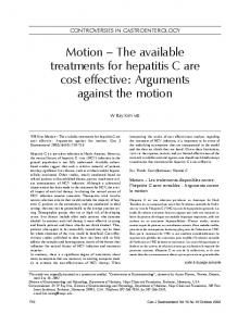
The overall error rate cannot be computed precisely unless the protocol for reviewing the results during the trial is explicitly specified. I guess that it is approximately 0.15. If the overall error rate had been reported rather than the nominal error rate (0.0369) in 2002, then the conclusion that HRT increases the risk of CHD might not have been regarded as statistically significant; the result might not have been published; thousands of women on HRT might not have been panicked; and the study might not have been terminated. • The basic approach to evaluating the strength of evidence might be changed to a likelihood approach. The parameter which indexes alternative hypotheses for this example is the relative risk of CHD for women on HRT compared to the risk of HRT for women on placebo. The continuous line on Figure 1 shows the likelihood of alternative hypotheses relative to the null hypothesis that HRT has no effect on CHD using the 2002 version of the data. The most likely relative risk is 1.286. Its likelihood is 8.98 times as large as that of the null hypothesis that the relative risk is 1. For the 2003 version of the data, the likelihood ratio is shown on Figure 1 as a dotted line. The maximum likelihood is 5.21 for a relative risk of 1.223.
Likelihood relative to null hypothesis
10.0 5.0
2.0 1.0 0.5
0.2 0.1 1.0
1.2
1.4
1.6
1.8
Relative risk of CHD associated with HRT
Figure 1: Likelihood of data in Table 3 as a function of the relative risk. The continuous line gives the likelihood based on the data available in 2002 when the study was terminated, and the dotted line gives the likelihood based on all of the data in 2003.
The Akaike Information Criterion suggests that the maximum likelihood ratio should be reduced by a factor of e = 2.718 to take into account the fact that the null hypotheses is a simple hypothesis whereas the alternative hypothesis is a one-parameter family of hypotheses. Particularly if they are modified using the Akaike Information Criterion, the maximum likelihood ratios do not seem to provide strong evidence against the hypothesis of no effect. Certainly the strength of evidence is less than a likelihood ratio of 19:1, which might be naively thought to somehow correspond to a P-value of 0.05. 10
• A Bayesian approach might be used for evaluating the strength of evidence. This would obviously not be an objective way to evaluate the strength of evidence because the apparent strength of evidence depends on the prior distribution used. One prior distribution which might be used is a flat prior for the log relative risk. Such a prior might be regarded as representing ignorance about the relative risk. For this prior, the posterior probability that the true effect of HRT on CHD is advantageous is 0.0179 for the 2002 data and 0.0344 for the 2003 version of the data. These numbers are similar to one-sided P-values for Fisher’s exact test. Such similarity between the results of Bayesian and Frequentist methodologies is sometimes taken to indicate that in situations like this the differences between schools of thought don’t matter very much. Another possible prior is that the log relative risk has an atom with probability 0.8 at zero and the remaining 0.2 probability is normally distributed with mean 0.1 and standard deviation 2. This might have been the prior subjective belief of the people conducting the trial in that it has a substantial probability of no effect and the conditional distribution of any non-zero effect is fairly uncertain with a slight bias towards the effect being deleterious. For the 2002 version of the data, the corresponding posterior distribution has probabilities 0.0072, 0.5972 and 0.3956 of the log relative risk being negative, zero or positive, respectively. For the 2003 version of the data, the posterior distribution of the log relative risk has probabilities 0.0091, 0.7347 and 0.2562 of being negative, zero or positive, respectively. Bayes factors defined as the posterior probability that the log relative risk is positive divided by the prior probability that the log relative risk is positive are 3.80 for the 2002 version of the data and 2.46 for the 2003 version of the data. Bayes factors are subjective measures of the strength of evidence. These Bayes factors suggest that the evidence for the relative risk being greater than unity is much weaker than the odds ratios of (1 − 0.0369)/0.0369 = 26.1 and (1 − 0.0771)/0.0771 = 12.0 which might be computed as strengths of evidence corresponding to the P-values.
It is not reasonable to expect that statistical inferences will be perfectly repeatable, given the variability of data, but it is reasonable to expect that statistical inferences with high reliability should seldom be contradicted by subsequent more reliable studies. Ioannidis (2005b) reviewed the reproducibility of some medical research results that might be expected to be quite reliable. He started with 115 published articles which all had more than 1000 citations. Of these, 45 articles made efficacy claims. For 14 of these articles (31%), subsequent studies that were either larger or better controlled either contradicted the findings (7 articles) or found that the effects were weaker than claimed (7 articles); for 20 articles (44%), subsequent studies replicated the results; and the claims of 11 articles (24%) remained largely unchallenged. He considered that the overall reproducibility of research findings was poor compared to the reproducibility which might have been expected from the P-values. Motulsky (2014) mentioned two other studies which found smaller proportions of studies to be reproducible. Young & Karr (2011) also discussed this problem. Collins & Tabak (2014) expressed several concerns about the poor reproducibility of biomedical research. Statistical analysis was not their primary focus, but they did state “Some irreproducible reports are probably the result of coincidental findings that happen to reach statistical significance, coupled with publication bias‘”and that “there remains a troubling frequency of published reports that claim a significant result, but fail to be reproducible.” 11
3.2
P-values not consistent with the Likelihood Principle
A second problem with P-values is that they are not consistent with the Likelihood Principle. The Likelihood Principle says that statistical conclusions should only be affected by the likelihood of the data actually observed. One way of justifying this principle is Bayesian. For any given prior distribution, the posterior distribution only depends on the likelihood. So even though you might not know which prior distribution is the correct one in any sense, your conclusion should only depend on the likelihood, not on the stopping rule or the probabilities of unobserved data. Birnbaum (1962) provided a non-Bayesian justification. See Berger & Wolpert (1984) for a thorough discussion of the history of the Likelihood Principle with many examples. In the discussion of Birnbaum (1962), Pratt gave a memorable intuitive justification of the Likelihood Principle. An engineer measures some voltages, obtaining data ranging from 75 to 99 volts. After analysing the data, a statistician notices that the volt-meter reads only as far as 100. Any data exceeding 100 would have been “censored”, so a new analysis appears to be required. The engineer also has a high-range volt-meter, equally accurate and reading to 1000 volts, which he at first says that he would have used if any voltage had been over 100; so new data analysis is not required. He later realizes that it was not working the day the experiment was performed, and admits that he would not have held up the experiment until the meter was fixed. The statistician concludes that the new data analysis will indeed be required. The engineer retorts “But the experiment turned out just the same as if the high-range meter had been working. I obtained the precise voltages of my sample anyway, so I learned exactly what I would have learned if the high-range meter had been available. Next you’ll be asking about my oscilloscope.” One of the logical consequences of the Likelihood Principle is the Stopping Rule Principle: that the evidence provided by the final data from a sequential experiment does not depend on the stopping rule. See Berger & Wolpert (1984, page76). Frequentist methods do not satisfy the Stopping Rule Principle. Experimenters using Frequentist methodology to analyse their data ought to take into account whether they stopped experimenting because the data appeared to be providing strong evidence for or against their null hypothesis; or because their money, their source of suitable subjects, or their enthusiasm had run out. They should consider the experimenters’ original intentions and how they would have reacted to all of the possible data that might have arisen. This seems to be a non-objective and very unfortunate feature of Frequentist methods. It is illustrated by Examples 3.2.1 and 3.2.2. Example 3.2.1. Consider testing between the two simple hypotheses H0 that X has a standard normal distribution and H1 that X is normally distributed with mean 1 and standard deviation 1. We will compare three possible experiments. ¯ > 0.6. Experiment 1 is that 8 independent observations are made and H0 is rejected if X This Neyman–Pearson test has Type I error rate 0.0448 and Type II error rate 0.1289. Experiment 2 is that 18 independent observations are made and H0 is rejected if ¯ > 0.6. This Neyman–Pearson test has Type I error rate 0.0055 and Type II error rate X 0.0448. Experiment 3 is a two-stage sequential test. First, 8 independent observations are ¯ > 0.8, H0 is rejected; and if X ¯ < 0.3, H1 is rejected. If 0.3 ≤ X ¯ ≤ 0.8, made. If X then an additional 10 independent observations are made. Then using the mean of all ¯ > 0.6. This two-stage test has Type I error rate 0.0150 observations, H0 is rejected if X and Type II error rate 0.0533. ¯ = Within the Neyman–Pearson approach of hypothesis testing, consider observing X 0.801 after 8 observations. If this is part of Experiment 1 then the Type I error rate 12
would be quoted as 0.0448. but if it is part of Experiment 3 then the Type I error rate ¯ = 0.73 after would be quoted as 0.0150. Consider also a set of observations such that X ¯ = 0.601 after 18 observations. The Type I error rate to be quoted 8 observations and X is about 3 times as large if there had been intent to examine the data after 8 observations than if there had been no such intent. ¯ = 0.65 after 18 Within Fisher’s approach to hypothesis testing, consider observing X observations. If this is under the protocol of Experiment 2 then the P-value would be ¯ after 8 0.0029. However if it was under the protocol of Experiment 3 (the value of X observations being such that the second stage of observation was undertaken), then the P-value will be larger because it includes some probability that the experiment would ¯ > 0.8 at the have been terminated after the first stage. If all of the probability that X completion of the first stage is added then the P-value is 0.0133. If only the probability ¯ > 0.8375 at the completion of the first stage is added (on the grounds that the that X likelihood ratio at the end of the first stage exceeds the 14.880 corresponding to the final data) then the P-value is 0.0104. Both of these possible P-values are much larger than if the data had been observed as part of Experiment 2. For both styles of hypothesis testing, the P-value for outcomes with the same likelihood ratio varies from one experiment to another. Barnard (1947b) gave the following illustration of how P-values appear to be affected by stopping rules, based on a letter from R.A. Fisher. Example 3.2.2. Suppose that 10 chrysanthemum seeds were planted. The null hypothesis is that half will produce white flowers and half will produce purple flowers. Let p denote the probability that a seed grows to maturity. If 9 seeds grow to maturity and produce purple flowers, then the outcomes which are as likely or less likely than the observed outcome are 9 white & 0 purple, 0 white & 9 purple, 10 white& 0 purple, and 0 white & 10 purple. The total probability of these four outcomes under the null hypothesis is 10p9 (1 − p)(2−9 + 2−9 ) + p10 (2−10 + 2−10 ) = (p/2)9 (20 − 19p) which has a maximum value of 0.002401 at p = 18/19. This number might be quoted as a P-value. On the other hand, if all seeds were viable but one plant was killed by a statistician while running for a bus, the experiment may be analysed as if the intention had been to grow 9 plants. The outcomes which are as likely or less likely than the observed outcome are 9 white & 0 purple, and 0 white & 9 purple. Their total probability is 2−9 + 2−9 = 0.003906 and this number might be quoted as a P-value. This analysis would also be preferred by statisticians who condition on ancillary statistics, such as the number of seeds growing to maturity in this example.
3.3
P-values not coherent with Bayesian methods
If a prior distribution is known then Bayesian statistics provides the only sensible way to proceed. In such circumstances it is interesting to check whether P-values are coherent with Bayesian methods. Lindley (1957) presented a class of situations for which P-values can be badly in conflict with Bayesian posterior distributions. Such incoherence seems to be to be undesirable even if not all arguments for the necessity of Bayesianity are accepted. My personal reason for not being completely persuaded by the proofs that Bayesianity is necessary for conclusions to be coherent is as follows. 13
The logic of the proofs of the necessity of Bayesianity can be used to show that two people who must act jointly3 should act as if they had a consensus prior. The consensus prior can only depend on the priors of the two people (since all of their relevant knowledge is subsumed into their priors), so there must be a rule for computing a consensus prior from two priors. This rule ought to satisfy two conditions. 1. Taking the consensus prior before seeing some data then using that prior to compute a consensus posterior should give the same result as seeing the data before taking the consensus. Therefore the rule for taking a consensus must be based on taking a weighted average of log odds. 2. If two points in the parameter space have exactly the same likelihood for all possible data then these two points can be collapsed into one (e.g. the moon is made of yellow cheese and θ = 4 and the moon is made of blue cheese and θ = 4). Collapsing the parameter space before or after taking the consensus should give the same result. This consistency condition is only satisfied if the rule for taking a consensus is to take a weighted average of prior probabilities. Now the only rules for taking a consensus that satisfy both of these conditions are to use A’s prior and completely ignore B’s, to use B’s prior and completely ignore A’s, and to use a third person’s prior and completely ignore both A’s and B’s priors. None of these options is satisfactory if Bayesian methods are to be used for scientific inference. This argument leads me to believe that Bayesian statistics does not provide an ultimate answer to the question of how to do statistical inference. However, I still like the Bayesian paradigm because it has the good feature that its weaknesses are readily visible. Consider now the following situation which is similar to many common simple statistical analyses. Example 3.3.1. Suppose that a single observation, X, is normally distributed with unknown mean, µ, and unit standard deviation. The null hypothesisis is that µ = 0. If X = 2, then the Frequentist approach might reject the null hypothesis and quote the P-value Pr[|X| ≥ 2] = 0.0455 as a measure of the reliability of this conclusion. Consider a Bayesian prior distribution which gives probability 0.8 to H0 and the remaining 0.2 prior probability to a probability distribution that µ is normally distributed with mean 0.1 and standard deviation 2. For X = 2, the Bayesian posterior distribution has probability 0.6346 for H0 and probability 0.3654 that µ is normally distributed with mean 1.52 and standard deviation 0.8944. The two-sided P-value of 0.0455 is not in direct contradiction with the posterior probability of 0.6346 that H0 is true, because the P-value is only a statement about the probability distribution of X under H0 and this statement is indeed true. However, insofar as the P-value is interpreted as giving any sort of indication as to what we might believe after seeing the data then it is not coherent with the posterior distribution. And for other prior distributions, the posterior probability the H0 is true could be higher or it could be lower. This example illustrates the point made in Section 1.1 that P-values are answering a question which is different from assessing strength of evidence or belief. It is somewhat similar to Example 3.1.1 if the parameter µ is interpreted as the logarithm of the relative risk. The prior distribution could be interpreted as saying that there was a substantial prior probability that hormone replacement therapy does not affect the rate of coronary heart disease, and that any actual effect, if non-zero, was uncertain and slightly more likely to be deleterious than advantageous. 3
Utilities can be specified so that all joint actions are better than all non-joint actions, thereby forcing the two people to act jointly if they wish to maximize their individual utility.
14
3.4
P-values not coherent with Likelihood methods
Quoting the entire likelihood function is always a very good way of summarizing the evidence provided by data. This is not a practical way to proceed for large parameter spaces, but is very satisfactory for comparing two simple hypotheses because the likelihood ratio is a single number. For comparing two simple hypotheses, the likelihood ratio is just as useful as the raw data for computing a posterior distribution. Examples 3.1.1, 3.2.1 and 3.3.1 all illustrate the fact that P-values are often not consistent with the likelihood ratio for tests between simple hypotheses. I regard this as a serious inconsistency because the likelihood ratio has a strong claim to being the only correct way to summarize the strength of evidence in such circumstances.4 In order to understand the relationship between the Likelihood and Bayesian approaches to inference, Royall (1997) suggests that it is useful to distinguish between the following three problems. 1. What evidence is there? 2. What should I believe? 3. What should I do? He argues that Likelihood methods should be used for problems of the first type, Bayesian methods for manipulating distributions of subjective opinion should be used for problems of the second type, and Bayesian methods with estimated utility functions should be used for problems of the third type. Example 3.4.1. As an illustration of the differences between these problems, suppose that a positive result for a blood test is 25 times as likely if a person has condition A as it would be if the person does not have condition A. The strength of evidence provided by such a positive result could be summarized by the likelihood ratio, 25. This answers Royall’s first question. However, suppose that the background proportion of people having condition A is 1 in 10000. Then after a positive test result is observed, the probability that the person has condition A is, by Bayes’s rule, 1 × 25/(1 × 25 + 9999 × 1) = 25/10024 ≈ 0.0025. This answers Royall’s second question. It would be unreasonable to believe that the person has condition A, but this is not as unlikely as it was before the test was conducted. Now, the expected utility should be calculated for each of the possible actions and the action of higher expected utility should be chosen in order to answer Royall’s third question.5 I consider that Royall’s wording of his first question is rather biased in that the second and third questions both include the word “I”, implying that the answers are expected to be subjective, but the absence of a pronoun in the first question implies that there is an 4
Note that this claim is not at odds with the idea that you have to be Bayesian to be coherent. For any Bayesian procedure for testing between two simple hypotheses, the Bayes factor is the same as the likelihood ratio. 5 If a standard treatment for condition A is cheap, is very effective, and has no side-effects then it would be appropriate to apply that treatment. Failing to treat might have higher expected utility if the standard treatment is expensive, not reliably effective, or frequently causes non-trivial side-effects — in which case there would have been little point to administering the blood test. In principle, expected utilities should be calculated from the point of view of the person being treated, but decisions by health workers are also influenced by risk of litigation and whether costs and potential future costs will be covered by insurance, government subsidies or other parts of the health system.
15
objective measure of the amount of evidence. For testing between two simple hypotheses, the likelihood ratio is indeed an objective measure of the amount of evidence, but more situations are more complicated and there is no such objective measure. Example 3.4.2. Another way in which two-region tests of hypotheses are not coherent with likelihood involves comparing the power of alternative experiments. Suppose X is normally distributed with standard deviation σ. Consider testing H0 that X has mean 0 against H1 that X has mean 1. Table 5 shows a range of tests which have chosen Type I error rates (which are essentially the same as P-values). The values for σ and for the cutoff xc have been chosen so that the Type II error rates are double the Type I error rates. This ratio has been chosen because it is common in practice for Type II error rates to be larger than Type I error rates. The power of the tests increases from 0.6 to 0.998 but the likelihood ratio in favour of H1 for data where H0 is just rejected increases only slightly: from 1.38 to 1.883. So for this range of experiments, data which just allows rejection of H0 for provides weaker evidence of essentially the same strength even though Frequentist measures of the power of the test vary over a very wide range between experiments. Table 5: Likelihood ratio in favour of H1 at cutoff for hypothesis tests with specified Type I and Type II error rates. Type I error rate 0.2000 0.1000 0.0500 0.0250 0.0100 0.0050 0.0025 0.0010
Type II error rate 0.400 0.200 0.100 0.050 0.020 0.010 0.005 0.002
Power 0.600 0.800 0.900 0.950 0.980 0.990 0.995 0.998
Likelihood ratio 1.380 1.595 1.702 1.765 1.817 1.843 1.863 1.883
A third way in which Fisher’s version of P-values is not coherent with likelihood is that censored data appears to provide the same strength of evidence as uncensored data. So far as I know, this criticism of P-values is novel. I consider this problem to be the crux of Example 3.4.2. The likelihood ratio gives the strength of evidence in favour of H1 provided by xc , whereas the Type I and Type II error rates are indicative of the strength of evidence which would be provided by a test in which the only data provided was whether X < xc or X ≥ xc . Example 3.4.3. As a stand-alone illustration of this issue using pure hypothesis testing, suppose that H0 is that X has a standard normal distribution and large values of X are to be regarded as rare. The censored observation X > 1.7 would be associated with a P-value of Pr[X ≥ 1.7 | H0 ] = 0.0446. The uncensored observation X = 1.7 would also be associated with a P-value of Pr[X ≥ 1.7 | H0 ] = 0.0436. However, the likelihoods of these two observation can be markedly different. For instance for the alternative hypothesis µ = 3, L[X ≥ 1.7 | µ = 3]/L[X ≥ 1.7 | µ = 0] = 20.27 whereas L[X = 1.7 | µ = 3]/L[X = 1.7 | µ = 0] = 1.82. 16
3.5
P-values allow relevant subsets
P-values can also be criticized because they sometimes allow the existence of relevant subsets. Robinson (1975) presented three artificial situations to illustrate this. For all of them, likelihood-based interval estimates give more sensible summaries of the available evidence than do interval estimates based on P-values (i.e. confidence intervals). Example 3.5.1. Figure 2 shows a modification of the third of those situations with the confidence interval, I(x), having 90% confidence. The region I(x) is the range covered by the bold lines. i.e. the region between F (x|θ) = 0 and F (x|θ) = 0.9. The region J(x) is the range covered by the light lines. i.e. the region between F (x|θ) = 0.9 and F (x|θ) = 1. Note that the lowest bold line and the highest light line both correspond to F (x|θ) = 0.9, so there is no probability that X will fall between them. Segments of all lines F (x|θ) = p have gradients 0.1 or 1.9. The value of ∂F (x|θ)/∂θ is 0.9 inside I(x) and is 0.01 inside J(x). Hence the probability densities are as indicated using text on Figure 2. Both X and θ may be negative, but only the positive quadrant is shown.
θ
7 6
Density = 1.71
5
Density = 0.09
4 3
Density = 0.001
2
Density = 0.019
1 0 0
1
2
3
4
x
5
Figure 2: An artificial one-dimensional family of distributions. The bold lines show F (x|θ) = p for p = 0, 0.1, 0.2, . . . , 0.9. The range, I(X), covered by these bold lines is a 90% confidence interval for θ. The light lines (of which there are 11 but only the first six are visible in the range shown) show F (x|θ) = p for p = 0.90, 0.91, 0.92, . . . , 1.00. The range covered by these light lines is referred to as J(X).
Take A to be the set of real numbers whose integer part is even. It corresponds to the bold line segments on the x-axis. Now I(X) is a 90% confidence interval which seems satisfactory according to Neyman (1937), but has quite poor conditional properties. We can see from the probability densities that Pr[X ∈ A & θ ∈ I(X) | θ] ≤ 0.09, Pr[X 6∈ A & θ ∈ J(X) | θ] ≤ 0.01. 17
Hence Pr[X 6∈ A & θ ∈ I(X) | θ] ≥ 0.81, Pr[X ∈ A & θ ∈ J(X) | θ] ≥ 0.09, Pr[θ ∈ I(X) | X ∈ A, θ] =
Pr[X ∈ A & θ ∈ I(X) | θ] Pr[X ∈ A & θ ∈ I(X) | θ] + Pr[X ∈ A & θ 6∈ I(X) | θ]
That the proposition θ ∈ I(X) is correct 90% of the time does not provide an adequate intuitive basis for “90%” to be a defensible measure of the reliability of the proposition θ ∈ I(X) after X has been observed. Given X ∈ A the proposition θ ∈ I(X) is true less than 50% of the time; and given X 6∈ A the proposition is true more than 98.78% of the time. Both the set A and its complement are relevant subsets. More crucially, A is called a negatively biased relevant subset because the probability that θ ∈ I(x) conditional on X ∈ A is always lower than the nominal value. Such a subset is regarded as a severe criticism because it means that confidence has been over-stated. When x ∈ A, the likelihood function is 0.09 for θ ∈ I(x) and is 0.019 for θ ∈ J(x). Since I(x) is of length 1 and J(x) is of length 10, a uniform (improper) Bayesian prior distribution for θ gives a posterior probability of 0.09/(0.09 + 0.19) = 0.3214 for θ ∈ I(x). When x 6∈ A, the likelihood function is 1.71 for θ ∈ I(x) and is 0.001 for θ ∈ J(x). The Bayesian posterior probability that θ ∈ I(x) is 1.71/(1.71 + 0.01) = 0.9942 for a uniform prior. These posterior probabilities are consistent with the conditional probabilities above. A likelihood approach to interval estimation might claim that I(x) is a reliable interval estimate for θ when x 6∈ A because the likelihood is 171 times larger for θ ∈ I(x) than for θ ∈ J(x). However a likelihood approach would not claim much reliability for I(x) as an interval estimate for θ when x ∈ A because the likelihood is 0.09/0.019 = 4.7 times larger for θ ∈ I(x) than for θ ∈ J(x).
3.6
P-values have other undesirable properties
P-values have a few undesirable properties apart from those already discussed. The following example illustrates the point that these undesirable properties can have important practical consequences. Example 3.6.1. Table 6 shows some data from an HIV vaccine trial in Thailand which was reported in Rerks-Ngarm et al. (2009). Only 51 out of 8197 people in the vaccine arm of the trial became infected with HIV, compared with 74 out of 8198 people who received a saline shot as a placebo. Using Fisher’s exact test for 2 × 2 tables, the P-level for a two-sided test is 0.0478 and the P-level for a one-sided test is 0.0239. The parameter which indexes the alternative hypotheses is the relative risk of HIV infection for people given the vaccine compared to the risk for people given the placebo. A likelihood-based analysis might report that the maximum relative likelihood is 8.52 for a relative risk of 0.816. It is not as high as the likelihood ratio of 10 which is advocated later in this paper as a possible minimum for a result to be regarded as “indicative”. The relative risks for which the likelihood is 1/19 of its maximum are 0.438 and 1.066. These 18
Table 6: Results from an HIV vaccine trial in Thailand Vaccine arm Placebo arm Total
Infected 51 74 125
Uninfected 8146 8124 16270
Total 8197 8198 16395
correspond to the same amount of statistical evidence as might be thought to be implied by a 95% confidence interval. This data set illustrates two common problems with P-levels. The first problem is the difficulty of choosing between one-sided and two-sided tests. Here the P-levels for onesided and two-sided tests are 0.0239 and 0.0478, respectively. Such P-levels commonly differ by a factor of approximately 2, yet it is sometimes not clear which should be used. Before the vaccine trial had been conducted, I imagine that it would have been considered very unlikely that the real risk of HIV was higher for the vaccine than for the placebo, so a one-sided tests seems appropriate. However it was not impossible that the vaccine might increase the risk, so many people would advise using a two-sided test. A trial designed to have a desired probability of rejecting the null hypothesis if the vaccine had some preconceived level of effectiveness would be quite a bit smaller if it was intended to use a one-sided significance test than if it was intended to use a two-sided significance test. It seems intuitively unreasonable that the amount of resources required to conduct such a trial should be so dependent on a somewhat arbitrary decision. The second problem which can be illustrated by this example is that under some circumstances, P-levels change abruptly as a function of the data. If there had been two extra people in the vaccine arm of the HIV vaccine trial and neither of them had become infected with HIV then the one-sided P-level would have only changed from 0.02394 to 0.02387 but the two-sided P-level would have changed from 0.0478 to 0.0393. This dramatic change occurs because for the original 2 × 2 table the probability of getting 51 HIV infections in the placebo arm (and therefore 74 infections in the vaccine arm since the analysis is proceeding as if the marginal totals in Table 6 are fixed) is slightly smaller than the probability of 51 HIV infections in the vaccine arm (and 74 in the placebo arm) so it is included in the two-sided P-level; but for the modified data the probability of getting 51 HIV infections in the placebo arm is slightly larger than the probability of 51 HIV infections in the vaccine arm so it is not included in the two-sided P-level. Such a dramatic change in P-value for a minor change in the data seems intuitively unreasonable. Table 7: Results from a hypothetical HIV vaccine trial
Vaccine arm Placebo arm Total
Infected 1 7 8
Uninfected 23 17 40
Total 24 24 48
Consider now the hypothetical set of results in Table 7 that could have arisen from a much smaller trial of the HIV vaccine. The two-sided and one-sided P-levels for Fisher’s exact test using this data are 0.0479 and 0.0240, respectively. They are almost the same as for the Thailand trial presented as Table 6. However, likelihood analysis gives a maximum relative likelihood of 19.74, which is much larger than the maximum relative likelihood of 19
8.52 for the Thailand trial. Likelihood-based analysis suggests that this hypothetical trial provides much stronger evidence against the null hypothesis than does the Thailand trial, despite P-value analysis suggesting that the strength of evidence is almost the same. This illustrates the point that changing from P-values to likelihood-based hypothesis tests would affect the relative apparent strengths of evidence by different amounts for different sets of results. It also illustrates the point that using likelihood ratios is not equivalent to taking a transformation of the P-level.
4
Comments on other people’s suggestions about what needs to be fixed
4.1
Avoiding hypothesis testing does not avoid the problems associated with P-values
Particularly in psychology, many people have advocated avoiding hypothesis testing and favouring the quoting of effect sizes and interval estimates. See Yates (1951), Carver (1978), Gardner & Altman (1986), Sterne & Smith (2001), Harlow et al. (1997) and Cumming (2012). I agree that interval estimates convey more information that hypothesis tests. Also, I have seen cases where statistical significance is claimed but the estimated effect size is very small and has not been mentioned because it would make the results seem less interesting. However, these preferences are just as relevant to Bayesian and likelihood data analysis regime as they are to Frequentist data analysis, so I consider that this argument is quite separate from arguments about the relative merits of different schools of statistical inference. Most of the arguments against P-values given above are as applicable for interval estimation as for hypothesis testing. In particular, quoting a confidence interval for the HRT data in Example 3.1.1 would have been essentially as bad as the hypothesis test.
4.2
The distinction between Fisher’s tests of significance and Neyman– Pearson hypothesis testing is a red herring
Lehmann (1986), Lehmann (1993), Hubbard & Bayarri (2003) and others have argued that the differences between Fisher’s and the Neyman–Pearson approach to hypothesis testing are important. I consider the following to be the two most important differences between these approaches. First, Fisher regarded the P-level as a function of the data whereas Neyman & Pearson (1933) regarded their measures of reliability (Type I and Type II error rates) as properties of an operational procedure. Second, Fisher’s approach deals with only a null hypothesis whereas Neyman and Pearson require that an alternative hypothesis be also specified. As a consequence of this difference Fisher’s approach does not provide a well-defined basis for choosing the statistic which is computed and assessed relative to its distribution under the null hypothesis, whereas Neyman–Pearson hypothesis tests are always based on a one-to-one function of the likelihood ratio. To understand the precise nature of some other differences seems to require a very careful reading of documents written by the protagonists. These differences are seldom important for applied statistics.6 6
One difference between the two approaches which is of practical importants is that Fisher (1956) argued that the Behrens–Fisher test for the two means problem is better than the Welch–Aspin test because there are negatively-biased relevant subsets for the Welch–Aspin test. The Welch–Aspin test aims to have approximately the nominal coverage probability, while Fisher viewed the Behrens–Fisher test as being based on his theory of fiducial probability (which had few adherents then and has virtually no adherents now). Fisher (1959, page 93) wrote “In fact, as a matter of principle, the infrequency with which, in particular circumstances, decisive evidence is obtained, should not be confused with the force,
20
Hypothesis testing in modern practice is usually a synthesis of the two approaches. The criticisms presented in section 3 are applicable to both approaches. In particular, the fact that statistical significance for the 2002 version of data for the hormone replacement therapy study (Example 3.1.1) seems to be an overstatement is applicable to both approaches.
4.3
That raising the barrier for “statistically significant” might alleviate the problem of poor reproducibility of apparently reliable results
Ioannidis (2005a) has suggested that the 5% P-level which is commonly used as a publication barrier is lower than is appropriate in medicine because it results in a large proportion of published results being later found to be substantially inaccurate. I agree that it is desirable to raise the barriers that must be passed before statistical evidence is considered to warrant a given amount of attention. The argument that P = 0.05 is much too low a barrier to be associated with the qualitative description “statistically significant” has been illustrated by a cartoon reprinted in Sterne & Smith (2001). It suggests that three wheels are spun in order to generate random propositions of the form A causes B in C (e.g. coffee causes depression in twins) which are then published in the New England Journal of Panic-Inducing Gobbledigook. This implies that associations reported in medical research are unreliable and vary from day to day. Some other people’s opinions about the cut-off values for P-values, likelihood ratios or Bayes factors which should be used in deciding whether a research paper in, say, medicine or psychology is worthy of publication are as follows. Fisher (1970, pages 80–81) suggested that P-values smaller than 0.01, 0.02 and 0.05 corresponded respectively to the null hypothesis being “definitely disproved”, that the null hypothesis “fails to account for the whole of the facts”, and that the data is “seldom to be disregarded”. Fisher (1926, page 504) says “Personally, the writer prefers to set a low standard of significance at the 5 per cent point, and ignore entirely all results which fail to reach this level.” Over many years, the interpretation of the P-value cutoff 0.05 has drifted from Fisher’s interpretation that results with P > 0.05 should generally be disregarded to being such that results with P < 0.05 are referred to “statistically significant”, suggesting that this is a level of evidence which is quite substantial. Fisher (1959, page 72) advocated likelihood ratio cutoffs of 2, 5 and 15. For situations like Example 4.3.1, below, these correspond approximately to P-values or error rates of 0.2, 0.1 and 0.02 for two-tailed tests or to P-values of 0.1, 0.05 and 0.01 for one-tailed tests. Jeffreys (1961, Appendix B) suggested that 100.5 should be the lower limit on the likelihood ratio for “substantial evidence”, 10 should be the lower limit for “strong evidence”, 101.5 should be the lower limit for “very strong evidence”, and 102 should be the lower limit for “decisive”. Royall (2000, page 761) cites Royall (1997) as providing a basis for a likelihood ratio of 8 being interpreted as “fairly strong evidence” and a likelihood ratio of 32 being interpreted as “strong evidence”. Kass & Raftery (1995) suggest that 3 be the lower limit for “positive” evidence, 20 be the lower limit for “strong” evidence, 150 be the lower limit for “very strong” evidence. In an unpublished but often cited paper, Evett (1991) argued that for forensic evidence alone to be conclusive in a criminal trial, the Bayesian posterior odds for guilt should be at least 1000. or agency, of such evidence”, indicating that he did not regard coverage probability as a particularly important property.
21
Considering these opinions and that there is always been pressure from researchers to overstate the reliability of results, I would like to suggest that a likelihood ratio of 10 be regarded as indicative, 100 be regarded as reliable, and 1000 be regarded as very reliable. Because these limits are expressed in terms of likelihood ratios and amounts of evidence are on a log-likelihood scale, these terms imply that reliable requires two times as much evidence as indicative and very reliable requires three times as much evidence as indicative. The simple situation that I presume Fisher (1959) had in mind when comparing the scale of P-values and the scale of likelihood ratios is as follows. Example 4.3.1. Suppose that X has a standard normal distribution with unknown mean µ and unit variance. The null hypothesis is that µ = 0 and the alternative hypothesis is that µ 6= 0. Let φ(.) denote the density function and let Q(.) denote the right hand tail area for the standard normal distribution. If we observe X = x > 0 then the P-value for a two-sided test is 2Q(x). The interval from 0 to 2x is a confidence interval with confidence level 1 − 2Q(x). The most likely parameter value for the alternative hypothesis is µ ˆ = x, so the likelihood ratio in favour of H1 is φ(0)/φ(x) = exp( 21 x2 ). The relationship between x and these measures of strength of evidence is shown in Table 8. One way to interpret them is that the P-values are the measures of reliability for the two-region hypothesis tests and the likelihood ratios are the measures of reliability for the three-region hypothesis tests. Table 8: P-values and likelihood ratios for hypothesis tests for Example 4.3.1 x 1.177 1.282 1.645 1.794 1.960 2.146 2.326 2.327 2.576 3.035 3.090 3.291 3.717
Using Table 8, my suggested likelihood ratio cut-offs of 10, 100 and 1000 might be translated into the suggestion that P-value cut-offs be 0.0032 for indicative, 0.0024 for reliable, and 0.0002 for very reliable. For Example 4.3.1 or for any other particular tightlydefined situation, the P-value is a 1-1 function of some statistic (here x) and the likelihood ratio is a 1-1 function of the same statistic. Therefore the P-value is a 1-1 function of the likelihood ratio. However, this relationship is generally different for other situations. Figure 3 shows four pairs of beta distributions. Figure 4 shows the relationships between the P-value and the likelihood ratio for these four pairs of beta distributions. We can 22
6 4 0
2
Probability density
8
10
see that there is a lot of variation from the continuous line which shows the relationship between the P-value and the likelihood ratio for Example 4.3.1 and the bold line which shows the relationship which might be naively assumed, namely P = 1/(1 + LR) where LR is the likelihood ratio.
0.0
0.2
0.4
0.6
0.8
1.0
x
Figure 3: Four pairs of families of beta distributions for hypothesis tests. The pairs are differentiated by using different line types: dotted, dashed, longdashed and dot-dashed. The cutoff-value for an hypothesis test with Type I and Type II error rates both being 0.05 is indicated by a vertical line of the same line type. The distribution to the left is the null hypothesis in each pair.
A practically important situation where there is variation from the standard relation¯ and s for ship between the P-value and the likelihood ratio is the t-test. If we observe X data from a normal distribution with unknown mean and variance then interval estimates ¯ − ts, X ¯ + ts) where the t valfor µ using a two-sided P-value of 0.05 are of the form (X ues are shown in Table 9. The likelihood ratios for such interval estimates vary with the number of degrees of freedom, as shown in Table 9. If the likelihood ratio is kept fixed at the value 10 then the corresponding t values are shown in Table 10. Now the P-values for such interval estimates vary with the number of degrees of freedom, as shown in Table 10. An even greater deviation from the standard relationship between the P-value and the likelihood ratio shown in Table 8 occurs for sequential tests. Figure 5 shows as a dashed line the relationship between P-value and likelihood ratio for a sequential test between the null hypothesis that the mean is 0 and the alternative hypothesis that the mean is 1. Observations are normally distributed with standard deviation 2. The test is terminated as soon as a likelihood ratio of 10 is observed. The graph is based on 10000 simulations. Figure 6 shows histograms of the likelihood ratios from the same 10000 simulations of a sequential test. It also shows the distribution of the likelihood ratio for a fixed test in which 44 observations are made. For this single-stage test the probabilities of Type I and Type II error are both 0.0486. These examples show that the relationship between P-values and likelihood ratios is different for different situations. And it is different for one-sided tests and two-sided tests. 23
0.99
P−value
0.975 0.95 0.9 0.8 0.5
0.2 0.1 0.05 0.025 0.01 0.005 0.001 0.001
0.01
0.1
1
10
100
Likelihood ratio in favour of alternative hypothesis
Figure 4: P-values as a function of likelihood ratio for families for hypothesis tests between the pairs of beta distributions shown in Figure 3. These relationships are shown using the same line types as in Figure 3. The bold sloped line shows where the P-value is 1/(1 + LR). The curve shown as a continuous line is the relationship for tests between normal distributions.
Table 9: Limits for confidence intervals based on a two-sided P-value of 0.05 for a tdistribution. The third column gives the non-centrality parameter corresponding to the P-value. The fourth column gives the likelihood ratio Degrees of freedom 1 2 3 5 10 30 100 ∞
t cutoff 12.706 4.303 3.182 2.571 2.228 2.042 1.984 1.960
Probability 19.32 14.38 11.93 9.80 8.24 7.27 6.96 6.83
Changing the cut-off P-values that are commonly used to define “significant” would solve part of the problem highlighted by Ioannidis (2005a), but would not solve all of it.
4.4
Selective reporting should be discouraged
Selective reporting is not necessarily relevant to a discussion of P-values, but other people have raised the topic of “P-hacking” while discussing P-values so I feel a need to address it. 24
Table 10: Limits for confidence intervals based on a likelihood ratio cutoff of 10 for a t-distribution. The third column gives the non-centrality parameter corresponding to the likelihood ratio. The fourth column gives the probability that the cutoff will be exceeded Degrees of freedom 1 2 3 5 10 30 100 ∞
t cutoff 6.577 3.543 2.960 2.588 2.352 2.212 2.165 2.146
Probability 0.0961 0.0713 0.0596 0.0490 0.0405 0.0347 0.0327 0.0319
0.99
P−value
0.975 0.95 0.9 0.8 0.5
0.2 0.1 0.05 0.025 0.01 0.005 0.001 0.001
0.01
0.1
1
10
100
Likelihood ratio in favour of alternative hypothesis
Figure 5: P-values as a function of the likelihood ratio. The dashed line is for a sequential test as described in the text. The bold sloped line shows where the P-value is 1/(1+LR) and the curve shown as a continuous line is the relationship for tests between normal distributions.
Motulsky (2014) uses the term “P-hacking” to include a variety of procedures for reanalysing data which might be tried “until you obtain a statistically significant result or until you run out of money, time or curiosity”. The cartoon on his page 202 (Reprinted from http://xkcd.com/882 under the CC BY-NC 2.5 license) illustrates the conducting of 20 experiments to investigate the possible relationship between eating jelly beans of particular colours and acne. One experiment found a “statistically significant” relationship between green jelly beans and acne when analysed as if that hypothesis had been the only one of interest before the set of experiments was conducted. The same cartoon was also reproduced in Young & Karr (2011). 25
600 500 400 300 0
100
200
Frequency
1/30
1/10
1/3
1
3
10
30
100
300
1000
Likelihood ratio
Figure 6: Distribution of likelihood ratios for fixed and sequential trials. The bold line shows the distribution under the null hypothesis of the likelihood ratio in favour of the alternative hypotheses. The lighter line shows the distribution under the alternative hypothesis of the likelihood ratio in favour of the alternative hypotheses. This histograms show distribution of the likelihood ratio for 10000 simulations of a sequential trial, with shading lines from topleft to bottom-right for the distribution under the null hypothesis and shading lines from top-right to bottom-leftt for the distribution under the alternative hypothesis.
Some alternative terminology is that Simmons et al. (2011) refers to researchers making decisions about amount of data, exclusion of some data, choice of control variables and data transformations as “researcher degrees of freedom”. Insofar as “P-hacking” or “researcher degrees of freedom” is used to mean looking at the data-to-date on several occasions and choosing to stop the data collection or experiment if the data so far supports some conclusion, I think that “P-hacking” is not merely acceptable but is a desirable practice. It should be accepted according to the Likelihood Principle. See section 5.4. Insofar as “P-hacking” is used to mean conducting many statistical tests and only reporting the ones that make the results look important, I call it “selective reporting” and believe that it is highly undesirable. An example of such selective reporting is that Cacioppo et al. (2013) says “The percentage of marital break-ups was lower for respondents who met their spouse on-line (5.96%) than off-line (7.67%) [ χ2 (1) = 9.95, P < 0.002]. Importantly, after controlling for year of marriage, to account for different follow-up times across respondents, and for sex, age, educational background, ethnicity, household income, religious affiliation, and employment status as covariates, this difference was attenuated but remained significant [χ2 (1) = 3.87,P < 0.05].” In their study there were substantial differences in the distributions of covariates be26
tween respondents who met their spouse on-line and respondents who met their spouse off-line. In my opinion, the first statistical analysis reported has essentially no value because it does not adjust for the covariates, while the second analysis is more appropriate. (For the second analysis the P-value is only just less than 0.05 so the evidence is very weak, as argued in the next section.) If I had been the reviewer of Cacioppo et al. (2013) then I think that I would have asked that the first analysis be omitted. However, all that I am asking my readers to accept is that to have reported only the first analysis would have been grossly misleading... and that a referee should know enough about analysis of covariance to know that the second analysis could be done and would be more appropriate even if the authors had not reported it. It is generally accepted that estimated effects should be adjusted for covariates when analysing observational studies. A classic example was given by Cochran (1968). The unadjusted death rates given in Table 11 suggest that smoking cigars and pipes is much more dangerous than smoking cigarettes. However, death rates are known to increase with age and the cigarette smokers were much younger than the cigar and pipe smokers. Adjusted death rates computed using 12, 8 and 11 age categories for the Canadian, British and U.S. studies, respectively, are also shown in Table 11. They are adjusted to the mean ages for non-smokers in each study separately. These adjusted data suggest that cigarette smoking is dangerous but cigar and pipe smoking is not.
Table 11: Death rates per 1000 person-years and mean ages for groups of men classified by smoking habit in three studies.
Smoking group Non-smokers Unadjusted death rate (Mean age) Adjusted death rate Cigarettes only Unadjusted death rate (Mean age) Adjusted death rate Cigars, pipes Unadjusted death rate (Mean age) Adjusted death rate
5
Canadian
Study British
U.S.
20.2 (54.9) 20.2
11.3 (49.1) 11.3
13.5 (57.0) 13.5
20.5 (50.5) 29.5
14.1 (49.8) 14.8
13.5 (53.2) 21.2
35.5 (65.9) 19.8
20.7 (55.7) 11.0
17.4 (59.7) 13.7
Suggestions for doing better
The aim of this paper is to argue that P-values are not a good measure of the reliability of a statistical analysis. It is desirable to give a better indication of reliability. In situations which are not pure significance testing, I believe that Likelihood and Bayesian methods are better. Approaches recommended for some particular types of situation are discussed below. 27
5.1
Deciding between two simple hypotheses
When testing between two simple hypotheses (which is not a common practical problem), I advocate using three-region hypothesis tests. This is equivalent to using likelihood ratios, which I believe to be the only sensible measure of the strength of evidence in these simple situations. Example 5.1.1. Largely following Berkson (1942, page 332), consider two sets of possible data from trials of a serological test designed to ascertain the gender of a fetus in utero. Let us compare a small experiment which gives the correct result 10 times out of 13 and a large experiment which gives the correct result 527 times out of 1000. Pure significance tests of the null hypothesis that the probability of a correct result is 0.5 give P-values of 0.0461 and 0.0468 for the small and large experiments, respectively. These P-values suggest that the strength of evidence is similar. For the small experiment, a two-region Neyman–Pearson test which rejects H0 whenever the number of correct results, X, is 10 or more has Type I error rate 0.0461 and Type II error rate 0.9071 if H1 is that the true proportion of correct results is 0.55 and 0.8314 if H1 is that the true proportion of correct results is 0.6. The corresponding test for the large experiment rejects H0 whenever X ≥ 527 has Type I error rate 0.0468 and Type II error rates 0.0678 if H1 is that the true proportion of correct results is 0.55 and 0.00000125 if H1 is that the true proportion of correct results is 0.6. The much larger Type II error rates for the small experiment indicate that it is much less reliable than the large experiment. Frequentist 90% confidence intervals for the true proportion of correct results are (0.505, 0.934) for the small experiment and (0.5005, 0.553) for the large experiment. These are consistent with rejection of the null hypothesis using one-sided hypothesis tests at P=0.05 and also give an indication of the greater informativeness of the large experiment. Three-region hypothesis tests using a likelihood ratio of 10 for the alternative hypothesis that the true proportion of correct results is 0.55 never make any conclusion for the small experiment. For the large experiment, the null hypothesis is accepted when X ≤ 513 and the alternative hypothesis is accepted when X ≥ 537. The probabilities of making the correct conclusion, no conclusion and the incorrect conclusion are approximately 0.804, 0.186 and 0.0103 whichever hypothesis is true. For the alternative hypothesis that the true proportion of correct results is 0.6, the cutoffs are 1 and 13 for the small experiment and 544 and 557 for the large experiment. The probabilities of making the correct conclusion, no conclusion and the incorrect conclusion are approximately 0.0015, 0.9983 and 0.00013 for the small experiment and approximately 0.9975, 0.0023 and 0.00018 for the large experiment. The three-region hypothesis tests seem to be satisfactory. Merely computing P-values is quite unsatisfactory because it suggests that rejections of the null hypotheis on the bases of the small and large experiments are approximately equally reliable.
5.2
Confidence intervals for location parameters
Another class of problem where I feel confident about the best method of data analysis is for location-parameter families of distributions. Suppose that they have probability densities of the form fθ,φ (x) = gφ (x − θ) for some function gφ . The parameter φ is known and we wish to estimate the parameter θ given a single observation X = x. If is often considered that Bayes and Frequentist approaches to inference are reliable in such circumstances because the Bayes approach with a uniform (improper) prior gives interval estimates which agree with Frequentist confidence intervals. The next two examples illustrate the point that interval estimates ought to both have 28
some guaranteed minimum probability content and include all parameter values for which the likelihood is within some multiple of its maximum. Example 5.2.1. Each member of this family of distributions is a convolution of a uniform distribution and a normal distribution which both have mean θ. The total variance is always unity. The parameter, φ, used to index these families is the standard deviation of the normal component. For θ = 0, an interval covering the central 95% of the distribution is from −cP to cP where cP is given in the third column of Table 12. The probability density at X = cP is smaller than at X = 0 by the multiplicative factors given in the fourth column of Table 12 which is headed “LR”. The point where the probability density is 1/10 of its maximum is cL . The probability content of the region from −cL to cL is given in the sixth column of Table 12. Table 12: Coverage and likelihood intervals for first set of location parameter families. When θ = 0, X is distributed as the convolution of a normal distribution with mean zero and standard deviation φ and a uniform distribution with mean zero and variance 1 − φ2 . Standard deviation of normal (φ) 1.00 0.80 0.60 0.40 0.20 0.10 0.05 0.01
Upper limit of uniform distribution 0.000 1.039 1.386 1.587 1.697 1.723 1.730 1.732
For given φ, interval estimates for the location parameter θ based on probability content are unsatisfactory if we interpret them as allowing us to reject hypotheses not included in the interval estimates. For instance for φ = 0.05, if we observed X = x then our interval estimate for θ would be from x − 1.644 to x + .644 but the just-rejected location-parameter value θ = x + 1.644 would have likelihood which was smaller than the maximum likelihood at θ = x by a factor of only 1.045. For smaller values of φ, the likelihood ratio can be made arbitrarily close to unity. Interval estimates based on a likelihood ratio cut-off seem satisfactory (conservative) from the point of view of probability content. For instance for φ = 0.05, if we observed X = 2 then our interval estimate for θ would be from x − 1.794 to x + 0.794. This has probability content Pr[θ ∈ (X − 1.794, X + 1.794)] = 0.9986. Example 5.2.2. Each member of this family of distributions is a mixture of two normal distributions which both have mean θ. The first component has probability φ and standard 2 deviation p σ1 = (2φ) . The first component has probability 1 − φ and standard deviation σ2 = (1 − 16φ5 )/(1 − φ). The total variance is always unity. For θ = 0, an interval covering the central 95% of the distribution is from −cP to cP wherecP is given in the fourth column of Table 13. The probability density at cP is smaller than at 0 by the multiplicative factors given in the fifth column of Table 13 which is headed “LR”. The point where the probability density is 1/10 of its maximum is cL . 29
Table 13: Coverage and likelihood intervals for second set of location parameter family. When θ = 0, X is distributed as a mixture of two normal distributions. The first com2 ponent has probability φ and standard deviation p σ1 = (2φ) . The second component has probability 1 − φ and standard deviation σ2 = (1 − 16φ5 )/(1 − φ). The mixture always has unit variance. φ
The probability content of the region from −cL to cL is given in the seventh column of Table 13. Interval estimates based on probability content are satisfactory (conservative) if we interpret them as allowing us to reject hypotheses not included in the interval estimates. For instance for φ = 0.05, if we observed X = x then our interval estimate would be from x − 1.988 to x + 0.988 and the just-rejected location-parameter value θ = x + 1.988 would have likelihood which was smaller than the maximum likelihood at θ = x by a factor of 41.849. However, interval estimates based on a likelihood ratio cut-off are not satisfactory from the point of view of probability content. For instance for φ = 0.05, if we observed X = 2 then our interval estimate would be from x − 0.969 to x + 0.969. This has probability content Pr[θ ∈ (X − 0.969, X + 0.969)] = 0.6725. For smaller values of φ the probability content of the likelihood-base interval estimate can be made arbitrarily small.
5.3
Testing a simple null hypothesis against a compound alternative hypothesis
Many simple statistical analyses are similar to testing the mean of a normal distribution with unit variance to see whether the mean, µ, is zero. For instance testing whether regression coefficients are different from zero and testing for independence in 2 × 2 tables using Fisher’s exact test are both farily similar to such testing. Therefore it is of substantial practical interest to look at this situation. It was previously discussed as Example 4.3.1. Example 5.3.1. If there is no reason to give special consideration to the possibility that µ = 0 then I suggest that likelihood-based interval estimates be used. For instance, if X = 2.1 then an interval estimate for µ such that the likelihood is at least 1/10 of its maximum is (0.046, 4.246). However, if we do wish to give special consideration to the possibility µ = 0 then it seems desirable to give a likelihood penalty the more complicated hypothesis. The 30
information criterion of Akaike (1974) is one way of doing this. Akaike (1974) argues that the maximum log likelihood over a k-dimensional space should be penalized by k. Our H1 that µ 6= 0 is a 1dimensional space so this means aa additive penalty of 1 for the log likelihood or a multiplicative penalty of a factor of e for the likelihood. For instance, if X = 2.1 then the likelihood of H0 that µ = 0 is 0.044. The maximum likelihood for H1 is 0.399 and the penalized likelihood is 0.147. This is not as much as 10 times as large as the likelihood for H0 , so we cannot reject H0 at the confidence level defined by a likelihood factor of 10. √ It can be argued that the likelihood penalty should only be a factor of e . When we observe X, the value ˆ = X, so the apparent maximum √ of µ which is most likely is µ likelihood of H1 is 1/ 2π. This is larger than the likelihood for the true µ by a factor of exp[ 21 (X − µ)2 ] Hence the expected apparent log likelihood ratio in favour of H1 exceeds the log likelihood ratio in favour of H1 for the true µ by E[ 21 (X − µ)2 ] = 12 . If this likelihood penalty penalty is used, then the value of X which just enables H0 to be rejected is 2.368. It should be noted that when such penalties are used for hypothesis testing, the interval estimate does not correspond to the set of parameter values which would not be rejected by hypothesis tests. I do not find this inconsistency abhorrent, unreasonable or even silly. Thinking within the Bayesian paradigm: different prior distributions might be used depending on whether the null hypothesis does or does not have an atom of probability in the prior distribution. See Berger & Delampady (1987). In general, I recommend that likelihood intervals be used for interval estimation7 but that penalized likelihood or Bayes factors be used for hypothesis testing. These are unlikely to be consistent with one another in the sense that it is common for a parameter value to be included in an interval estimate even though an hypothesis test would not reject that parameter value. For the HRT study (Example 3.1.1), there might be an additional penalty applied to the log likelihood of the alternative hypothesis in the spirit of multiple comparisons testing. Such an additional penalty would attempt to take into account the fact that several types of health outcome were being monitored. Schwarz (1978) proposed a criterion which is often referred to as the Bayesian Information Criterion (BIC). It amounts to penalizing the log likelihood by 12 k log(N ) where k is the dimensionality of the parameter space and N is the number of observations. Thel penalty proposed in Example 5.3.1 is the same as the BIC penalty for a one-dimensional parameter space but does not have a factor which depends on the number of observations. ¯ If we had N observations then we could construct an equivalent model in which Y = X 1 with variance 1/N was the only observation. The BIC gives a penalty of 2 log(N ) for the first model and a penalty of 21 for the equivalent model. This seems unsatisfactory, so I believe that the proposed penalty is more sensible that the BIC. Table 14 shows some values of the log likelihood ratio, the proposed penalized log likelihood ratio as LL−0.5, and the Akaike information criterion (AIC). The values of X have been chosen to correspond to particular one-sided P-values. Bayarri & Berger (1998, equation 2.1) have suggested that a P-value of p could be interpreted as approximately equivalent to a Bayes factor of −ep log(p) provided that p < e−1 . These approximate Bayes factors are tabulate in the column headed “BB approx.” They are numerically similar to the proposed penalized log likelihood ratios. This procedure for testing hypotheses proposed in Example 5.3.1 could be adopted as a standard technique for testing means of normal distributions. It is useful to have a standard technique because it makes people’s data analyses easier to understand. However 7
Though, as suggested in section 5.2, interval estimates should be made to have a certain minimum probability content also.
31
Table 14: Measures of support for alternative hypothesis X 1.645 1.960 2.326 2.576 3.090 3.291 3.719
in my view the technique has no claim to being objectively correct.
5.4
Sequential experimentation should be more common
So far in this section, the suggestions for doing better statistics by avoiding P-values have been concerned with data analysis. The last of the ways in which I think we could do better statistics is to make more use of sequential experimental design. Like Anscombe (1963), I think that this is very important. It woud lead to more efficient use of resources in a wide variety of investigations. As the first point of the summary of his criticism of Armitage (1975), Anscombe (1963) wrote “ Sequential analysis is a hoax”. He was endeavouring to express as emphatically as possible his belief that statistical analysis of sequential medical trials should only depend on the observed data, “and not on what might have been observed by wasn’t”. This attitude to data analysis comes with an attitude to conduct of sequential studies that it is acceptable to change the stopping rule at any time.
6 6.1
Discussion Describing strength of evidence for pure significance testing
For pure significance testing there seems to be no alternative to using P-values. However, I believe that the cut-offs for qualitative descriptions of statistical significance for pure significance testing should be changed to correspond approximately to those advocated in Section 5.3 for testing a normal mean. As indicated in Table 15, penalized likelihood ratios of 10, 100 and 1000 correspond to P-values of approximately 0.009, 0.0007 and 0.00006. In order to make them easier to remember, these might be rounded to 0.01, 0.001 and 0.0001. Using these cut-offs in pure significance testing would amount to a substantial increase in the strength of evidence required before standard qualitative statements are made about statistical significance.
6.2
Is it difficult?
Currently, most common statistical software is set up to compute P-values. This might make computing likelihood ratios and Bayes factors appear to be difficult. In principle, computing likelihoods is simpler than computing P-values, while computing Bayes factors is about as difficul as computing P-values. Difficulty of computing is not an adequate excuse for continuing to use P-values in situations where alternative hypotheses are specified. 32
Table 15: Cut-offs in support for alternative hypothesis Z 2.368 3.195 3.849
One-sided P-value 0.00895 0.00070 0.00006
Likelihood 16.5 164.9 1648.7
Penalized likelihood 10 100 1000
Qualitative descriptions indicative = positive evidence reliable =strong evidence very reliable = very strong evidence
Acknowledgements Much of this work was done while I was a Ph.D. student at University College London from 1972–1974. I was assisted and inspired by many visitors and staff, particularly Allan Birnbaum, A. Philip Dawid, Dennis Lindley and Mervyn Stone. I have also benefitted from discussions with colleagues at CSIRO, particularly Bill Venables. Some of this work was done using NIH funding under the supervision of Louise Ryan.
References Akaike, H. (1974). A new look at the statistical model identification. IEEE Transactions on Automatic Control 6, 716–723. Anscombe, F. J. (1963). Sequential medical trials. Journal of the American Statistical Association 58, 365–383. Arbuthnott, J. (1711). An argument for divine providence, taken from the constant regularity observ’d in the births of both sexes. Philosophical Transactions of the Royal Society 27, 186–190. Armitage, P. (1963). Sequential medical trials: Some comments on F.J. Anscombe’s paper. Journal of the American Statistical Association 58, 384–387. Armitage, P. (1975). Sequential Medical Trials. Blackwell Scientific, Oxford, 2nd ed. Barnard, G. A. (1947a). Book review of Sequential Analysis by Abraham Wald. Journal of the American Statistical Association 42, 658–664. Barnard, G. A. (1947b). The meaning of a significance level. Biometrika 34, 179–182. Bayarri, M. J. & Berger, J. O. (1998). Quantifying surprise in the data and model verification (with discussion). In Bayesian Statistics 6, J. M. Bernado, J. O. Berger, A. P. Dawid & A. F. M. Smith, eds. Oxford University Press, pp. 53–82. Berger, J. O. & Delampady, M. (1987). Testing precise hypotheses. Statistical Science 2, 317–335. Berger, J. O. & Wolpert, R. L. (1984). The Likelihood Principle: A Review, Generalizations, and Statistical Implications. Institute of Mathematical Statistics. Berkson, J. (1942). Tests of significance considered as evidence. J. Amer. Statist. Assoc. 37, 325–335. Birnbaum, A. (1962). On the foundations of statistical inference (with discussion). J. Amer. Statist. Assoc. 57, 296–306. Box, G. E. P. (1962). Sampling and Bayes’ inference in scientific modelling and robustness (with discussion). Journal of the Royal Statistical Society A 143, 383–430. Buehler, R. J. (1959). Some validity criteria for statistical inferences. The Annals of Mathematical Statistics 30, 845–863. Cacioppo, J. T., Cacioppo, S., Gonzaga, G. C., Ogbur, E. L. & VanderWeele, T. J. (2013). Marital satisfaction and break-ups differ across on-line and off-line meeting venues. Proc Natl Acad Sci U.S.A. 110, 10135–10140. 33
Carver, R. P. (1978). The case against significance testing. Harvard Educational Review 48, 378–399. Chernoff, H. & Scheffe, H. (1952). A generalization of the Neyman–Pearson fundamental lemma. The Annals of Mathematical Statistics 2, 213–225. Cochran, W. G. (1968). The effectiveness of adjustment by subclassification in removing bias in observational studies. Biometrics 24, 295–313. Collins, F. S. & Tabak, L. A. (2014). NIH plans to enhance reproducibility. Nature 505, 612–613. Cornfield, J. (1966). Sequential trials, sequential analysis and the likelihood principle. The American Statistician 20, 18–23. Cox, D. R. (2006). Principles of statistical inference. Cambridge University Press. Cox, D. R. & Hinkley, D. V. (1974). Theoretical Statistics. Chapman and Hall, London. Cumming, G. (2012). Understanding The New Statistics: Effect Sizes, Confidence Intervals, and Meta-Analysis. Routledge, New York. Dantzig, D. B. & Wald, A. (1951). On the fundamental lemma of Neyman and Pearson. The Annals of Mathematical Statistics 22, 87–93. Dempster, A. P. (1964). On the difficulties inherent in Fisher’s fiducial arguments. Journal of the American Statistical Association 59, 56–66. Evett, I. W. (1991). Implementing bayesian methods in forensic science. Paper presented at the Fourth Valencia International Meeting on Bayesian Statistics. Fisher, R. A. (1926). The arrangement of field experiments. Journal of the Ministry of Agriculture of Great Britain 33, 505–513. Fisher, R. A. (1956). On a test of significance in Pearson’s Biometrika Tables (No. 11). Journal of the Royal Statistical Society. Series B 18, 56–60. Fisher, R. A. (1959). Statistical Methods and Scientific Inference. Oliver and Boyd, Edinburgh, 2nd ed. Fisher, R. A. (1970). Statistical Methods for Research Workers. Oliver and Boyd, Edinburgh, 14th ed. Gardner, M. J. & Altman, D. G. (1986). Confidence intervals rather than P values: estimation rather than hypothesis testing. British Medical Journal 292, 746–750. Goodman, S. (2008). A dirty dozen: twelve p-value misconceptions. Seminars in Hematology 45, 135–140. Goodman, S. N. (2001). Of p-values and bayes: A modest proposal. Epidemiology 12, 295–297. Hacking, I. (1965). Logic of Statistical Inference. Cambridge University Press. Harlow, L. L., Muliak, S. A. & Steiger, J. H., eds. (1997). What If There Were No Significance Tests? Lawrence Erlbaum Associates Publishers. Hoenig, J. M. & Heisey, D. M. (2001). The abuse of power: The persuasive fallacy of power calculations for data analysis. The American Statistician 55, 1–6. Hubbard, R. & Bayarri, M. J. (2003). Confusion over measures of evidence (P’s) versus errors (α’s) in classical statistical testing. The American Statistician 57, 171–177. Hume, D. (1748). AN Enquiry Concerning Human Understanding. Ioannidis, J. P. A. (2005a). Contradicted and initially stronger effects in highly cited clinical research. Journal of the American Medical Association 294, 218–228. Ioannidis, J. P. A. (2005b). Why most published research findings are false. PLoS Medicine 2, e124. Jeffreys, H. (1961). Theory of Probability. Oxford University Press, 3rd ed. Johnson, D. H. (1999). The insignificance of statistical significance testing. Journal of Wildlife Management 63, 763–772. Kass, R. E. & Raftery, A. E. (1995). Bayes factors. Journal of the American Statistical Association 90, 773–795. 34
Klein, R. B. (2004). Beyond Significance Testing. Reforming data analysis methods in behavioral research. APA Books. Kuhn, T. S. (1970). The Structure of Scientific Revolutions. The University of Chicago Press, 2nd ed. Lambdin, C. (2012). Significance tests as sorcery: Science is empirical—significance tests are not. Theory & Psychology 22, 67–90. Langer, R. D., Manson, J. E. & Allison, M. A. (2012). Have we come full circle — or moved forward? The Womens Health Initiative 10 years on. Climacteric 15, 206–212. Lehmann, E. L. (1986). Testing Statistical Hypotheses. Wiley, New York, 2nd ed. Lehmann, E. L. (1993). The Fisher, Neyman–Pearson theories of testing hypotheses: One theory or two? Journal of the American Statistical Association 88, 1242–1249. Lindley, D. V. (1957). A statistical paradox. Biometrika 44, 187–192. Manson, J. E., Hsia, J., Johnson, K. C., Rossouw, J. E., Assaf, A. R., Lasser, N. L., Trevisan, M., Black, H. R., Heckert, S. R., Detrano, R., Strickland, O. L., Wong, N. D., Crouse, J. R., Stein, E. & Cushman, M. (2003). Estrogen plus progestin and the risk of coronary heart disease. The New England Journal of Medicine 349, 523–534. Motulsky, H. J. (2014). Common misconceptions about data analysis and statistics. The Journal of Pharmacology and Experimental Therapeutics 351, 200–205. Neyman, J. (1937). Outline of a theory of statistical estimation based on the classical theory of probability. Philosophical Transactions of the Royal Society of London. Series A 236, 333–380. Neyman, J. & Pearson, E. S. (1933). On the problem of the most efficient tests of statistical hypotheses. Philosophical Transactions of the Royal Society of London. Series A 231, 289–337. Pearson, K. (1900). On the criterion that a given system of deviations from the probable in the case of a correlated system of variables is such that it can be reasonably supposed to have arisen from random sampling. Philosophical Magazine, Series 5 50, 157–175. Rerks-Ngarm, S., Pitisuttithum, P., Nitayaphan, S., Kaewkungwal, J., Chiu, J., Paris, R., Premsri, N., Namwat, C., de Souza, M., Adams, E., Benenson, M., Gurunathan, S., Tartaglia, J., McNeil, J. G., Francis, D. P., Stablein, D., Birx, D. L., Chunsuttiwat, S., Khamboonruang, C., Thongcharoen, P., Robb, M. L., Michael, N. L., Kunasol, P. & Kim, J. H. (2009). Vaccination with ALVAC and AIDSVAX to Prevent HIV-1 infection in Thailand. The New England Journal of Medicine 361, 2209–2220. Robinson, G. K. (1975). Some counterexamples to the theory of confidence intervals. Biometrika 62, 155–161. Rossouw, J. E., Anderson, G. L., Prentice, R. L., LaCroix, A. Z., Kooperberg, C., Stefanick, M. L., Jackson, R. D., Beresford, S. A. A., Howard, B. V., Johnson, K. C., Kotchen, J. M. & Ockene, J. (2002). Risks and benefits of estrogen plus progestin in healthy postmenopausal women: Principal results from the Women’s Health Initiative randomized controlled trial. Journal of the American Medical Association 288, 321–333. Royall, R. (2000). On the probability of observing misleading evidence. Journal of the American Statistical Association 95, 760–768. Royall, R. M. (1997). Statistical Evidence: A Likelihood Paradigm. Chapman and Hall, New York. Schwarz, G. (1978). Estimating the dimension of a model. The Annals of Statistics 6, 461–464. Simmons, J. P., Nelson, L. D. & Simonsohn, U. (2011). False-positive psychology: Undisclosed flexibility in data collection and analysis allows presenting anything as 35
significant. Psychological Science 22, 1359–1366. Sterne, J. A. C. & Smith, G. D. (2001). Sifting the evidence—what’s wrong with significance tests? British Medical Journal 322, 226–31. Todhunter, I. (1949). A History of the Mathematical Theory of Probability from the Time of Pascal to that of Laplace. Chelsea Pub. Co., New York. Wagner, D. H. (1969). Nonlinear functional versions of the Neyman–Pearson lemma. SIAM Review 11, 52–65. Wallis, W. A. (1980). The statistical research group, 1942–1945. Journal of the American Statistical Association , 320–330. Yates, F. (1951). The influence of Statistical Methods for Research Workers on the development of the science of statistics. Journal of the American Statistical Association 46, 19–34. Young, S. S. & Karr, A. (2011). Deming, data and observational studies. a process out of control and needing fixing. Significance , 116–120.