Array and Multiport Antenna Farfield Simulation using EMPIRE, MATLAB and ADS S. Otto ∗1 , S. Held ∗2 , A. Rennings +3 , K. Solbach ∗4 (HFT) and + Allgemeine und Theoretische Elektrotechnik (ATE) University of Duisburg-Essen, Bismarck-Straße 81, 47057 Duisburg, Germany
∗ Hochfrequenztechnik
1
[email protected]
Abstract—This paper presents an efficient farfield simulation, exploiting and linking the strength of three commercial simulation tools. For many practical array and multiport antenna designs it is essential to examine the farfield for a general port excitation or termination scenario. Some examples are phased array designs, problems related to mutual coupling and scan blindness, tuning of parasitic elements, MIMO antennas and correlation. The proposed method fully characterizes the nearfield and the farfield of the antenna, so to compute farfield patterns by means of superposition for any voltage/current state at the port terminals. A recently published low-cost patch antenna phased array with analog beam steering by another group was found very suitable to demonstrate the proposed method.
I. I NTRODUCTION In many practical antenna design procedures it is required to analyze the farfield of a multiport antenna or an antenna array under different feeding conditions or for different termination scenarios. If the antenna structure itself is not modified, except for different excitation and termination states, a circuitsimulation based farfield superposition is possible, hence reducing the simulation time and allowing fast optimization in a circuit simulator. This concept has already been proposed in [1], [2] and [3] for various applications. Our work further introduces the dual farfield decomposition in terms of a voltage-farfield-basis and its relation to the current-farfieldbasis as proposed in [1]. The focus of this paper is the actual implementation using commercial software tools. Here we present a procedure which utilizes the three softTM R ware packages: EMPIRE (IMST), MATLAB (The Mathworks, Inc.) and ADS (Agilent Technologies) in the following manner: A full-wave FDTD simulation in EMPIRE for each port is performed. A postprocessing in MATLAB scans all relevant terminal and farfield data and decomposes the farfield. The decomposition of the farfield into a farfield-basis allows the combination to form the overall farfield for an arbitrary terminal states. Finally, the circuit simulation in ADS is used to setup external circuitry (feedings/loadings/reactive elements) and to compute the voltages and currents at all port terminals. After this simulation ADS triggers MATLAB to superimpose the farfields for this new state and reads back the final result. II. M ULTIPORT A NTENNAS A very general multiport antenna configuration is depicted in Fig. 1. An n-port antenna system is shown with its terminal quantities, voltages and currents as well as the farfield quantity.
An arbitrary number of antenna or radiating elements is possible using this very general approach. In case of closely spaced elements or a single antenna element with two or more ports, a strong coupling is evident and must be taken into account. In the following, the mathematical method is presented in detail. We define the electric field ~E as shown in Fig. 1 as the electric farfield with no field component in propagation direction. In this region (Fraunhofer region) the field components are essentially transverse and the angular distribution is independent of the radial distance where the measurements are made [4]. Furthermore, the absolute field strength in V/m is computed for the distance r = 1 m, so to deal with an absolute farfield quantity, which is no restriction. For the angle depended farfield on a sphere with the radius r = 1 m we have: ~E := ~E(r = 1 m, θ , ϕ)
(1)
z
u1
~ E
r
i1
y
i2
u2
x in
i3
u3 Fig. 1.
un
Multiport antenna with n-ports and the radiated electric farfield ~E.
III. FARFIELD D ECOMPOSITION The electric farfield ~E can be decomposed into terms of a contribution from each of the n ports. We furthermore define ~ 1, . . . , K ~ n which results a farfield-current-basis for each port K in the total farfield when multiplied with the port currents: ~E = K ~ 1 i1 + K ~ 2 i2 + · · · + K ~ n in
(2)
~ has the same θ and ϕ angle dependency as ~E The quantity K ~ = V . To solve for the n farfields K ~ 1, · · · , K ~n and is of unit [K] m·A
farfield data:
E
(4a) (4b)
terminal data:
.. . ~En = K ~ 1 i1,n + K ~ 2 i2,n + · · · + K ~ n in,n
V
[n × n] [n × n]
(4c) Fig. 2.
⇒
KI or
[1]
MV [n × 1]
~ ϕ) E(θ,
I or V
s-parameter Touchstone
file.snp
Using a compact matrix notation we have E = IK,
I
[1 × n]
ADS AC Circuit
iterations
~E1 = K ~ 1 i1,1 + K ~ 2 i2,1 + · · · + K ~ n in,1 ~E2 = K ~ 1 i1,2 + K ~ 2 i2,2 + · · · + K ~ n in,2
n simulations:
decomposition into K or M
The overall system of linear equations is given in (4) with ~E1 , . . . , ~En the electric farfields for the corresponding port excitation 1, . . . , n.
MATLAB
EMPIRE FDTD reading Empire data
we need n linear independent equations. In order to generate this independent set of equations each port is excited with all other ports terminated with loads. The following indexing of currents and voltages is used to refer to the excitation and to the monitoring: imonitoring,excitation (3)
Flow chart for the circuit based farfield superposition.
(5)
with the two column vectors of the fields E and K and the current matrix I,
IV. I MPLEMENTATION AND E XAMPLE : PATCH A NTENNA ARRAY
E = (~E1 , ~E2 , · · · , ~En )T ~ 1, K ~ 2, · · · , K ~ n )T K = (K i1,1 i2,1 · · · in,1 i1,2 i2,2 · · · in,2 I= . .. .. .. .. . . . i1,n i2,n · · · in,n
In [5] a low cost electronically steerable patch antenna array with two passive radiators is presented. All the related data can be found in that publication. Using this example, the here proposed farfield superposition method will be explained and validated. In Fig. 2 a schematic flowchart shows the function and the data flow of the three software packages used.
(6b)
(6c)
In an equivalent manner the field E can be decomposed into a voltage-farfield-basis with E = VM
6 mm
(7)
with V the voltage-matrix (same indexing as I) and the farfieldmatrix M corresponding to K. Furthermore, we can find the admittance-matrix Y and impedance-matrix Z using the following relation: IT = YVT and VT = ZIT
35 mm y
28.3 mm
(6a)
(8)
If the multiport antenna system is passive and reciprocal, the impedance and admittance matrix are both symmetric. The relation between the voltage-farfield-basis and current-farfieldbasis is therefore: V−1 (YT V)T K = YK = M
(9)
K = ZM
(10)
Either K or M has to be computed, with the other quantity calculated by using the impedance or admittance matrix. The decomposition of the overall farfield into terms of a current-farfield-basis (same as in [1]) or voltage-farfield-basis is mathematically equivalent, so either of these can be chosen. In some applications one or the other is more useful and gives a better physical insight, e.g. dipoles might be modeled using currents, whereas for radiating slots voltages are more suitable.
z
port 1
port 2
port 3
x
Fig. 3. Geometry of the patch array under investigation. Material parameters for the substrate are taken from 60-mil-thick Rogers RO3003, with εr = 3.
A. FDTD simulation: Empire A simulation model of the antenna presented in [5] has been setup in Empire, Fig. 3, to compute the terminal as well as the farfield quantities. The patches are placed in close proximity, thus a strong mutual coupling occurs. If only the center patch with port number 2 is fed and the outer parasitic patches with port numbers 1 and 3 are terminated with capacitors, beam steering has been achieved by varying the capacitances. For this n = 3 port antenna three EM simulations must be performed so to acquire the data needed to solve (5) and compute the current-farfield-basis K. Each port is excited and the voltages and currents as well as the farfield (this port excited all others terminated with loads) are stored in a separate sub-folder. The folder ”sub-1” holds the frequency
domain port voltages u f 1, u f 2, u f 3 and the frequency domain currents i f 1, i f 2, i f 3 as well as the 3D-farfield data for the excitation of port 1, Fig. 4.
Fig. 5.
Structure type in MATLAB for the farfield ~E1 , with port 1 excited.
Fig. 4. Directory layout of EM-simulation data. Each ”sub-n” folder holds the simulation data for the corresponding excition of port number n.
B. Reading simulation data and computing farfield basis: MATLAB The folders ”sub-1”, ”sub-2”, . . . , ”sub-n” are postprocessed using MATLAB. First, all data is read into an object type structure, Fig. 5. Shown here is ~E1 with the corresponding voltages and currents for the port excitation 1. The Θ-component of the electric farfield ~E is stored in the variable etheta with an angle increment of 3◦ resulting in a 121 × 61 MATLAB array. The ϕ-component is stored in ephi, respectively. Next, MATLAB solves equation (5) for all angles θ and ϕ to compute the current-farfield-basis K. The same object type ~ 1 , shown in Fig. 6. For K ~1 in MATLAB is use to represent K all currents are zero, except for the i1 = 1, so to form the basis ~ 2 and K ~ 3. with K
~ 1 , the Fig. 6. Structure type in MATLAB for the current farfield basis K calculated farfield for i1 = 1, i2 = 0 and i3 = 0.
The pre-processing has been done in EMPIRE and MATLAB to compute the current-farfield-basis as describe in Sec. IV-A. The port numbering here is ascending with the driven center element having the port number 2. The outer patches are connected to ground through a capacitor C1 at the first patch element and a capacitor C3 at the third patch element. AC
C. Circuit Simulation and Simulation Iteration: ADS & MATLAB The s-parameter data is imported as Touchstone file into ADS. Voltage and current monitors are placed at the terminals as shown in Fig. 7. The antenna is excited with AC power source and the monitored terminal currents are written to a file. By means of a system-call in the measurement equations MATLAB is triggered to read the new current file from ADS and superimpose the farfields. After this completion the calculated farfields are read back to ADS for further evaluation like visualization, optimization or tuning. The farfield simulation is now purely circuit based and thus very efficient. In Fig. 2 this fast iteration procedure is shown by the highlighted dashed box. V. VALIDATION : PATCH A RRAY WITH PARASITIC R ADIATORS The patch antenna array is simulated with the proposed method and the results are compared to the ones obtained in [5]. The dimension and material properties are taken from [5].
u1
2
1 3
AC AC1 Start=1 GHz Stop=5 GHz Step=
u1 I_Probe I_Probe1 C C1 C=C1 pF
Var Eqn
Meas Eqn
u2
Ref
u3 S3P SNP2 File="empire_exported_touchstone_file.s3p"
u2 I_Probe I_Probe2 P_AC PORT1 Num=1 Z=50 Ohm Pac=polar(dbmtow(0),0) Freq=freq
u3 I_Probe I_Probe3 C C3 C=C3 pF
VAR VAR2 file_name="nf2ff_1_f3.00000e+009_MATLAB_eabs" dir_file_name=strcat("..\\..\\ff_data\\", file_name) file_upd_plot=strcat("..\\ff_data\\", file_name) MeasEqn Meas3 wv_ib=write_var("..\\..\\ff_data\\I_ads_output.txt","W","", " ", "f",10, freq, I_Probe1.i, I_Probe2.i, I_Probe3.i) opsys1=system( "super_pos", FALSE, "", TRUE) result=read_matlab_file_1(dir_file_name) xz=ff_plane(result,"Phi",0)
Fig. 7. ADS schematics; the MeasEqns invoke Matlab and read the results back into ADS.
For the values of C1 = 0.2 pF and C3 = 1.0 pF, an angle of θ = +20◦ and for C1 = 1.0 pF and C3 = 0.2 pF, an angle of θ = −20◦ was observed by the authors of [5].
Var Eqn
Goal OptimGoal1 Expr="dB(xz)" SimInstanceName="AC1" Min=10 Max=10 Weight=1 RangeVar[1]="Theta" RangeMin[1]=-21 RangeMax[1]=-21
10 9 8 7 6 5 4 3 2 1 0 -1 -2 -3 -4 -5 -6 -7 -8 -9 -10
Var Eqn
ph0_pol
GOAL
VAR VAR24 C1=0.2 {t} {o} C3=0.2 {t} {o}
10 9 8 7 6 5 4 3 2 1 0 -1 -2 -3 -4 -5 -6 -7 -8 -9 -10
ph0_pol
Var Eqn
VAR VAR24 C1=0.2 {t} {o} C3=1 {t} {o}
VAR VAR24 C1=1 {t} {o} C3=0.2 {t} {o}
Theta (-180.000 to 180.000)
Fig. 8. Directivity (linear plot) for the three different pairs of capacitance values to validate the calculation with the results in [5]
We used our method to simulate the farfield patterns for these two configurations. In Fig. 8 the total directivity pattern, based on the electric field was calculated and plotted in ADS. The maximum directivity was found at θ = ±21◦ (our angle step is 3◦ ) which is in very good agreement with the results presented in [5]. It could be observed that the maximum directivity at broadside is lower than the directivity at θ = ±21◦ . In [5] only normalized directivity values are given, which is of course totally sufficient to support their good and efficient concept for a low cost steerable antenna array. A comparison of the actual directivity is therefore not possible here. Nevertheless, without going into the details of the small directivity drop at broadside, we present a directivity optimization using the ADS environment, pointing out the advantages of the farfield superposition method. An optimization goal was defined in ADS where we set the goal value of the directivity for the required beam pointing angle of the antenna to D = 10 dB, as indicated by the GOAL in Fig. 9 for an angle of Θ = −21 dB. The results have been obtained within a fraction of time compared to a full-wave EM optimization and the values are summarized in Tab. I. It can be seen that the directivity still slightly drops (approx. 0.1 dB) at broaside. Neverthess, it was possible to find optimized capacitance pairs for a constant maximum directivity over the whole scanning range. The return loss is not shown here, there was good impedance matching for all beam pointing directions. VI. C ONCLUSIONS A very versatile method for efficient and fast farfield superposition based on circuit simulation data has been presented. Many practical problems can be addressed where different excitation and/or termination states of the antenna ports are of interest. Furthermore, virtual ports could be used in an antenna to gain a better physical insight or to systematically design couplings or aperture distributions. The three software tools: EMPIRE, MATLAB and ADS have been available to us and are very suitable for the functionality needed. Nevertheless,
Theta (-180.000 to 180.000)
Fig. 9. Directivity (linear plot) for the optimized capacitance values of Tab. I: θ = [0◦ , −6◦ , −12◦ , −21◦ ] (due to symmetry only negative θ angles are evaluated) TABLE I D IRECTIVITY OPTIMIZATION FOR DIFFERENT BEAM ANGLES
angle θ (degree) 0 -3 -6 -9 -12 -15 -18 -21
directivity D (dB) 9.63 9.61 9.58 9.56 9.56 9.58 9.64 9.68
capacitance values C1 (pF) C3 (pF) 0.616 0.618 0.648 0.557 0.657 0.473 0.660 0.377 0.666 0.282 0.68 0.188 0.715 0.100 0.780 0.100
the superposition methodology based on the decomposition is of course not restricted to the software tools chosen here for our actual implementation. The implementation itself is not optimized with still file-based communication between the tools. Communication interfaces like COM or pipes/sockets offer a great potential for improvements. Unfortunately, for the AC circuit simulation they are not available in ADS. Only the DSP potelomy simulation comes with a MATLAB communication interface. R EFERENCES [1] K. Karlsson, J. Carlsson, I. Belov, G. Nilsson, and P.-S. Kildal, “Optimization of antenna diversity gain by combining full-wave and circuit simulations,” in Proc. Second European Conference on Antennas and Propagation EuCAP 2007, 11–16 Nov. 2007, pp. 1–5. [2] J. Carlsson and K. Karlsson, “Analysis and optimization of multi-port antennas by using circuit simulation and embedded element patterns from full-wave simulation,” in Proc. IEEE Antennas and Propagation Society International Symposium AP-S 2008, 5–11 July 2008, pp. 1–4. [3] K. Karlsson and J. Carlsson, “Circuit based optimization of radiation characteristics of single and multi-port antennas,” in Proc. 3rd European Conference on Antennas and Propagation EuCAP 2009, 23–27 March 2009, pp. 1513–1516. [4] C. A. Balanis, Antenna Theory: Analysis and Design, 2nd ed. Wiley, May 29 1996. [5] Y. Yusuf and X. Gong, “A low-cost patch antenna phased array with analog beam steering using mutual coupling and reactive loading,” IEEE Antennas Wireless Propag. Lett., vol. 7, pp. 81–84, 2008.