mobile wireless cellular networks. Cellular networks are rapidly growing around the ... Finally,. STP can reduce co-channel and adjacent channel interference.
Array Processing for Mobile Communications A. Paulraj and C. B. Papadias
1 Introduction and Motivation This section reviews the applications of antenna array signal processing to mobile wireless cellular networks. Cellular networks are rapidly growing around the world and a number of emerging technologies are seen to be critical to the improved economics and performance of the networks; among these is the use of multiple antennas and spatial signal processing at the base station. This technology is sometimes also referred to as smart antennas or perhaps more accurately as space-time processing (STP), since the antenna outputs are processed in space and time to maximize signal reception. A cellular network is used in a number of mobile/portable communications applications. Cell sizes may range from large macrocells, which serve high speed mobiles, to smaller microcells or very small picocells, which are designed for outdoor and indoor pedestrian tra�c, respectively. Each of these o�ers di�erent channel characteristics, and therefore, poses di�erent challenges for STP. Likewise, di�erent service delivery goals such as voice, data or video also need speci c STP solutions. STP in general provides three processing leverages. The rst is array gain. Multiple antennas capture more signal energy, which can be combined to improve the signal-to-noise ratio (SNR). Next is spatial diversity to combat space-selective fading. Finally, STP can reduce co-channel and adjacent channel interference. The organization of this chapter is as follows. In Section 2, we describe the vector channel model for a base station antenna array. In section 3 we discuss the algorithmic approaches in STP. Section 4 outlines the applications of STP in cellular networks. Finally, we conclude with a summary in Section 5. 1
2 Vector Channel Model for Base Station Antennas The propagation environment in cellular networks is complicated by multipath e�ects and user mobility. These circumstances create special challenges for STP; a thorough understanding of channel characteristics is the key to developing successful STP methods. The main features of mobile wireless channels are described below.
2.1 Propagation Loss and Fading
The radiated signal from the mobile su�ers power losses as it travels to the base station. These losses arise from the mean propagation loss and from slow and fast fading. The mean propagation loss comes from square law spreading, absorption by foliage and vertical multipath. A number of good models exist for characterizing the mean propagation loss [12, 16]. The loss is usually around 40 dB per decade. Slow fading results from shadowing by buildings and natural features and is usually characterized by a log-normal distribution with � = 8 dB. Fast fading results from multipath scattering in the vicinity of the moving mobile. It is usually Rayleigh distributed. However, if there is a direct path component present, the fading is better approximated by a Rician distribution.
2.2 Multipath E�ects
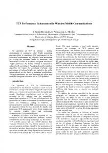
Multipath propagation plays a central role in determining the nature of the channel. By channel we mean the impulse, or frequency response, of the radio channel from the mobile to the output of the antenna array. We refer to it as a vector channel, since we have multiple antennas, and we therefore have a collection of channels. The mobile radiates omnidirectionally in azimuth using a vertical E- eld antenna. The transmitted signal then undergoes scattering, re ection, or di�raction before reaching the base station, where it arrives from di�erent paths, each with its own fading, propagation delay, and angle-of-arrival. This multipath propagation, in conjunction with user motion, determines the behavior of the wireless channel. Multipath scattering arises from three sources. See Figure 1. There are scatterers local 2
to the mobile, remote dominant scatterers, and scatterers local to the base. We will now describe these three scattering mechanisms and their e�ect on the channel. Scatterers Local to Mobile
Scatterers Local to Base Remote Scatterers
Figure 1: Multipath propagation has three distinct classes, each of which gives rise to di�erent channel e�ects
2.2.1 Scatterers Local to Mobile
Scattering local to the mobile is caused by buildings in the vicinity of the mobile (a few tens of meters). Mobile motion and local scattering give rise to Doppler spread, which causes time-selective fading. For a vertical, polarized E- eld antenna, it has been shown [12] that the fading signal has a characteristic classical spectrum. For a mobile traveling at 55 MPH, the Doppler spread is about +/- 200 Hz in the 1900 MHz band. This e�ect results in rapid signal uctuations also called time-selective fading. While local scattering contributes to Doppler spread, the delay spread will usually be insigni cant because of the small scattering radius. Likewise, the angle spread will also be small.
3
2.2.2 Remote Scatterers
The emerging wavefront from the local scatterers may then travel directly to the base or may scatter toward the base by remote dominant scatterers, which then gives rise to specular multipath. These remote scatterers can be terrain features or high rise buildings. Remote scattering can cause signi cant delay and angle spreads. Delay spread causes frequency-selective fading, and the angle spread results in space-selective fading.
2.2.3 Scatterers Local to Base
Once these multiple wavefronts reach the base station, they may be scattered further by local structures such as buildings or other structures that are in the vicinity of the base. Such scattering will be more pronounced for low elevation below-roof-top antennas. The scattering local to the base can cause severe angle spread. Delay δ 1
x θ
1
fading
Subscriber
path amplitude 1
θ x
path amplitude L
Delay δ
x
L
fading L
Figure 2: Multipath model
4
L
Base Station Antenna Array
x
Environment Delay Spread Angle Spread Doppler Spread Flat Rural (Macro) 0.5 �sec 1 deg 190 Hz Urban (Macro) 5 �sec 20 deg 120 Hz Hilly (Macro) 20 �sec 30 deg 190 Hz Microcell (Mall) 0.3 �sec 120 deg 10 Hz Picocell (Indoors) 0.1 �sec 360 deg 5 Hz Table 1: Typical delay angle and Doppler spreads in cellular applications.
2.3 Typical Channel Parameters
Measurements in macrocells indicate that up to 6 to 12 paths may be present. Typical channel delay, angle and one sided Doppler (1800 MHz) spreads are given below in Table 1.
2.4 Vector Channel Model
A multipath channel is illustrated in Figure 2. Typical path power and delay statistics can be obtained from the GSM standard. See Table 2 for an extract for the Hilly Terrain (HT). The angle-of-arrival is a random variable obtained by using scattering-point ellipsoids that assume equi-probable location of the remote dominant scatterers on a delay-de ned ellipse. A typical example of a mobile macrocellular channel is shown in Figure 3. We show a frequency response at each antenna for a GSM system . Since the channel bandwidth is high (200 KHz) the channel is highly frequency-selective in a hilly terrain environment. Also, the large angle spread causes variations of the channel from antenna to antenna. The channel variation in time depends upon the Doppler spread. Notice that since GSM uses a short time slot, the channel variation during the time slot is negligible. 1
1
Global System for Mobile communications.
5
Tap Relative Average Relative Doppler Number Time (�sec) Power (dB) Spectrum 1 2 3 4 5 6 7 8 9 10 11 12
(1)
(2)
(1)
(2)
0.0 0.1 0.3 0.5 0.7 1.0 1.3 15.0 15.2 15.7 17.2 20.0
0.0 0.2 0.4 0.6 0.8 2.0 2.4 15.0 15.2 15.8 17.2 20.0
-10.0 -8.0 -6.0 -4.0 0.0 0.0 -4.0 -8.0 -9.0 -10.0 -12.0 -14.0
-10.0 -8.0 -6.0 -4.0 0.0 0.0 -4.0 -8.0 -9.0 -10.0 -12.0 -14.0
Classical Classical Classical Classical Classical Classical Classical Classical Classical Classical Classical Classical
Table 2: Typical path amplitude, delay, and time selective fading spectrum for hilly terrain.
6
6
4
−6
−6
−6
−8
0.5
1
1.5
2
2.5 3 frequency
3.5
4
4.5
−10 0
5
1.5
2
2.5 3 frequency
3.5
4
4.5
−10 0
5
−8
0.5
1
1.5
2
5
x 10
2.5 3 frequency
3.5
4
4.5
−10 0
5
6
4
4
4
4
2
2
−2
−4
−4
−4
−6
−6
−6
−6
−8
0.5
1
1.5
2
2.5 3 frequency
3.5
4
4.5
−10 0
5
−8
0.5
1
1.5
2
5
x 10
2.5 3 frequency
3.5
4
4.5
−10 0
5
1
1.5
2
2.5 3 frequency
3.5
4
4.5
−10 0
5
6
6
4
4
4
4
2
2
−4
−4
−4
−6
−6
−6
−6
0.7
−8
−8
−8
−8
0.5
1
1.5
2
2.5 3 frequency
3.5
4
4.5
−10 0
5
0.5
1
1.5
2
5
x 10
2.5 3 frequency
3.5
4
4.5
−10 0
5
3.5
2.5 3 frequency
3.5
2.5 3 frequency
3.5
4.5
5 5
x 10
1
1.5
2
4
4.5
5 5
x 10
−2
−4
0.8
−10 0
2.5 3 frequency
4
0
−2
0.9
0.6
3.5
2
0
|H| (dB)
|H| (dB)
0
−2
0.5
5
x 10
6
0
2.5 3 frequency
−8
0.5
5
x 10
6
−2
2
−2
−4
−8
1.5
0
|H| (dB)
−2
1
2
0
|H| (dB)
0
−2
0.5
5
x 10
6
|H| (dB)
|H| (dB)
1
6
−10 0
|H| (dB)
−8
0.5
5
x 10
6
2
Hilly Terrain 1
|H| (dB)
−6
|H| (dB)
|H| (dB)
|H| (dB)
−4
2
λ/2
2
0
−2
−4
0
λ/2
4
2
0
−2
−4
−8
λ/2
6
4
2
0
−2
−4
−10 0
30
6
4
2
0
|H| (dB)
6
−2
0.5
1
1.5
2
5
x 10
2.5 3 frequency
3.5
4
4.5
−10 0
5
0.5
1
1.5
2
5
x 10
4
4.5
5 5
x 10
0.5 0.4 0.3
6
6
6
6
4
4
4
4
2
2
2
2
0.2
0 0
4
6
8
10 Delay (us)
12
14
16
18
20
0
−2
0
|H| (dB)
0
−2
|H| (dB)
|H| (dB)
2
|H| (dB)
0
0.1
−2
−2
−4
−4
−4
−4
−6
−6
−6
−6
−8
−10 0
−8
0.5
1
1.5
2
2.5 3 frequency
3.5
4
4.5
−10 0
5
−8
0.5
1
5
x 10
0 msec
1.5
2
2.5 3 frequency
3.5
4
4.5
−10 0
5 5
x 10
0.0666msec
−8
0.5
1
1.5
2
2.5 3 frequency
3.5
4
4.5
−10 0
5 5
x 10
0.1333msec
0.5
1
1.5
2
4
4.5
5 5
x 10
0.2msec
Figure 3: Channel frequency response at four di�erent antennas for GSM in a typical hilly terrain channel at 1800 MHz. Mobile speed is 100 KPH. The response is plotted at four time instances spaced 66 �secs. In IS-54 channels, because of the narrow signal bandwidth (30 KHz), the channel is much less frequency-selective, but channel variation during a slot is signi cant, since the time slot is much larger (6.66 ms). 2
2.5 Array Signal Model
The received baseband signal xi(t) at the i-th element of an m element antenna array is given by
xi(t) =
L X l=1
gi(�l)�l(t)u(t ? �l)
(1)
where L is the number of multipaths, gi (�l) is the response of the i-th element for an l-th path from direction �l, �l(t) is the complex envelope of the path fading, �l is the path delay, and u(:) is the transmitted signal that depends on the modulation waveform and the information data stream. In the above model we have assumed that the inverse signal bandwidth (the channel fading bandwidth is negligible in comparison) is large compared to the travel time across the array. Therefore, the signal complex envelope Interim Standard 54: the new version of this American TDMA standard for mobile communications is called IS-136. 2
7
received by each antenna is identical except for phase (and perhaps amplitude) di�erences that depend on path angle-of-arrival. This angle-of-arrival dependent phase shift is included in gi (�l) along with any amplitude-phase response di�erences for each element [23]. We can collect all the element responses to a path from angle �l into an m-dimensional vector. We call this the array response vector. Assuming there are m elements
a(�l) = [g (�l) g (�l) : : : gm(�l)]T 1
2
We can rewrite the array output as
x(t) = where
L X l=1
a(�l)�l(t)u(t ? �l)
(2)
x(t) = [x (t) x (t) : : : xm(t)]T 1
2
x(t) and a(�l) are m-dimensional complex vectors. The signal fading enve-
lope �(t) is typically Rayleigh or Rician distributed. If the fading is Rayleigh distributed, a reasonable frequency-spectrum model is either a classical spectrum or a at spectrum [12].
2.5.1 Spatial Structure
The spatial structure is given by the array manifold (AM), which is a set of array response vectors indexed by the angles-of-arrival and is depicted in Figure 4. The array manifold a(�) represents the response of the antenna elements relative to the rst element for a wavefront arriving at the carrier frequency from a direction �. The AM includes the e�ect of a number of factors, such as array geometry, element patterns, inter-element coupling, scattering from antenna support structures and other local scatterers near the base station. The AM, when measured at the receiver baseband, is also a�ected by receiver gain/phase response, which is usually frequency dependent within the passband of a single radio channel passband, I-Q (in-phase - quadrature phase) imbalance in the processor and other A/D converter-related errors. The AM is, of course, strongly dependent upon the channel frequency which 8
spans 25 MHz in the cellular band (824-849 MHz) and 60 MHz in the PCS band (1850-1910 MHz). Drifts in the receiver electronics and in external mechanical scattering structures can cause signi cant changes in the AM making it important to calibrate the AM frequently.
2.5.2 Temporal Structure
The transmitted signals u(t) also have temporal structure. For example the GMSK waveform has a constant modulus (CM) structure, since it has the general form (see Fig. 4)
u(t) = ej� t
( )
where �(t) is a Gaussian- ltered output of the phase of a minimum shift keyed (MSK) signal [24]. Another important temporal structure in mobile communications signals is the nite alphabet (FA). This structure underlies all digitally modulated schemes. The modulated signal is a linear or nonlinear map of an underlying nite alphabet. The IS-54 signal is given by
u(t) =
X
X
p
p
Apg(t ? pT ) + j Bpg(t ? pT )
Ap = cos(�p) Bp = sin(�p) �p = �p? + ��p 1
Array Manifold
Constant Modulus
Finite Alphabet
Figure 4: Spatial and Temporal Structure 9
(3)
where g(�) is the pulse shaping function (a square root cosine function in the case of IS-54), and ��p is chosen from a set of phase shifts f � ; � ; � ; � g depending on the data s(:). 5 4
3 4
4
7 4
2.6 Interference Model
TDMA cellular networks use a cellular layout with frequency reuse to support a large number of geographically dispersed users. When a mobile operates in a neighboring co-channel cell in the same frequency channel and time slot as the current user, co-channel interference will be present. The signalto-interference power ratio (SIR), also called the protection ratio, depends on a number of factors that include the reuse factor (J) (see [13]), propagation environment, mobile location and transmit power. It can be shown [7] that the protection ratio is 18:7 dB for J = 7, 13:8 dB for J = 4 and 11:3 dB for J = 3. In sectored cells, co-channel interference is signi cant mainly from cells within the sector. 3
2.7 Overall Array Data Model
The overall signal-plus-interference-and-noise model at the base station antenna array can now be rewritten as
x(t) =
L X l=1
a(�l)�l(t)u(t ? �l) +
Lq QX ?1 X q=1 l=1
a(�ql)�ql(t)uq (t ? �ql) + n(t) (4)
where the double sum term is the interference signal from Q ? 1 interferers and n(t) is the additive thermal noise. The distribution of all the parameters in Eq. (4) is as discussed above. We now sample x(t) at the symbol rate. If the delay spread-plus-symbol waveform duration is NT , the discrete array output can be written as
x(k) = Hsss (k) +
QX ?1 q=1
Hq sq (k) + n(k)
(5)
where Hs is a m � N matrix whose j -th column (j = 1; : : : ; N ) is given by 3
Time Division Multiple Access.
10
[Hs]j =
L X l=1
a(�l)�lg((j ? nl)T ? � ? �l)
(6)
where nl and � are parameters that depend on the sampling point and path delay. Hs represents the combined e�ect of symbol waveform and channel, and ss is a column vector of data given by 3
2
ss(k) 7 6 ... 7 (7) ss(k) = 64 5 ss(k ? N + 1) Hq and sq are accordingly de ned. Note that we have assumed the spacetime channel to be time-invariant. This is a reasonable assumption over time intervals that are substantially smaller than the inverse Doppler spread. If we collect M consecutive snapshots of x(�) corresponding to time instants k; : : :; k + M ? 1, and neglect for a moment the interference we get
X(k) = HS(k) + N(k)
(8)
where X(k), S(k) and N(k) are de ned as X(k) = [x(k) � � � x(k + M ? 1)]
(m � M )
S(k) = [ss(k) � � � ss (k + M ? 1)]
(N � M )
N(k) = [n(k) � � � n(k + M ? 1)] (m � M ) and we have dropped subscript s from H for convenience. Note that S(k) is
a Toeplitz data matrix. Equation (8) is the general linear data model that will be used throughout the chapter. It expresses the received signals as a convolution of the transmitted data and the channel. In space-time ltering, we use a space-time lter or equalizer W (see Fig. 5) that has the following form 2
3
w (k) � � � w M (k) 7 6 ... 7 = [w (k) � � � wM (k)] 6 W(k) = 4 ... � � � 5 wm (k) � � � wmM (k) 11
1
1
1
11
(9)
In order to obtain a convenient formulation for the ST- lter output, we introduce the quantities W (k) and X (k) as follows X (k) = vec (X(k)) (mM � 1) (10) W (k) = vec (W(k)) (mM � 1) where the operator vec(�) is de ned as: 2
vec ([v � � � vM ]) = 1
6 6 4
3
v
1
...
vM
7 7 5
The scalar equalizer output y(k) can be written as
y(k) = W H (k)X (k) (11) Having described the signal and interference model, we can now study how the output of the antenna array can be processed to maximize signal demodulation performance.
3 Algorithms for Array Processing The history of array signal processing goes back nearly four decades to adaptive antenna combining techniques using phase-lock loops for antenna tracking. An important beginning was made by Howells [11], when he proposed the sidelobe canceller for adaptive nulling and later Applebaum developed a feedback control algorithm for maximizing SINR. Another signi cant advance was the LMS algorithm proposed by Widrow [30]. Yet another important milestone was the work of Capon who proposed an adaptive antenna system [6] using a look direction constraint that resulted in the minimum variance distortionless beamformer. Further advances were made by Frost [8] and Gri�ths and Jim [9] among several others. See [28] for a review on spatial ltering through beamforming. Because of signi cant delay spread in the channel, array processing in mobile communications can be greatly leveraged by processing the array signals in space and in time (STP) to minimize both co-channel interference and inter symbol interference while maximizing signal to noise ratio. See Qureshi [22] for a review of channel equalization. 12
3.1 Single-User Algorithms
We begin with the single-user case where we are only interested in demodulating the signal of interest. We therefore treat interference from other users as unknown additive noise.
3.1.1 ML and MMSE
The rst criterion for optimality in STP is Maximum Likelihood (ML) or usually referred to as Maximum Likelihood Sequence Estimation (MLSE). MLSE seeks to estimate the data sequence which is most likely to have been sent given the received vector signal. Another frequently used criterion is Minimum Mean Square Error (MMSE). In MMSE we obtain an estimate of the transmitted signal as a space-time weighted sum of the received signal and seek to minimize the mean square error between estimate and the true signal. We outline ST-MLSE and ST-MMSE which are the ST extensions of the well known ML and MMSE algorithms.
ST-MLSE With the channel model described by Eq. (8), we assume that the noise N is spatially and temporally white and Gaussian, and that there is no interference. The ST-MLSE problem can be shown to reduce to nding S so as to satisfy the following criterion min (12) S kX ? HSkF where the channel H is assumed to be known and k:kF denotes Frobenius norm. This is a generalization of the standard MLSE problem where the channel is now de ned in space and in time. We can therefore use a ST generalization of the well known Viterbi algorithm (VA) to carry out the search in Eq. (12) e�ciently. See [21] for a discussion on VA method. The structure of a ST-MLSE can be seen in Figure 5. 2
4
ST-MMSE In applications when interference is present, we will not, in general, have 4
The channel H can be estimated using training sequences or blind techniques.
13
knowledge of the interference statistics. We can therefore no longer use MLSE and an alternative approach is MMSE. In MMSE we seek to nd a space-time lter (STF) (see Eq. (9)) that linearly combines the array output such that the di�erence between its scalar output and the true signal is minimized. The ST-MMSE criterion is therefore
2
min E
W H X (k) ? s(k ? D)
(13) W where D is a delay chosen to center the STF. The solution to this LS problem follows from the well known projection theorem 2
�
This leads to
�
E X (k)(X H (k)W ? s�(k ? D)) = 0 n
�
W = E X (k)X H (k)
�o?1
E (X (k)s�(k ? D))
(14) (15)
where superscript � denotes complex conjugate. If the interference and noise are independent of the signal, the transmitted bit sequence is white, and M >N 3 2 0 7 6
E (X (k)s�(k ? D)) =
6 6 6 6 6 6 6 6 6 6 4
�
0 vec (H) 0
�
7 7 7 7 7 7 7 7 7 7 5
=H
(16)
0 � � De ning the space-time mM � mM covariance matrix Rxx = E XX H , Eq. (15) takes the familiar form (17) W = R?xx H Note that when M = N , H = vec (H). A number of techniques are available in order to solve Eq. (17). A well known recursive algorithm is the least mean square (LMS) algorithm [30]. Other recursive techniques include the recursive least square (RLS) [15]. If we explicitly calculate R?xx and then use H to nd W , the approach is called Sample Matrix Inversion (SMI). There are a number of trade-o�s 1
1
14
between SMI, LMS, and RLS approaches that span numerical stability, convergence speed, and computational complexity. See [15] for a discussion. The ST-MMSE structure can be seen in Figure 5. Having seen the basic approaches for STP, we will now review techniques for implementing MLSE and MMSE. We divide these into non-blind and blind methods.
3.1.2 Non-Blind or Training Signal Methods
In many mobile communications standards such as GSM and IS-54, explicit training signals are inserted inside the TDM data bursts. These training signals can be used to estimate the channel needed for the ST-MLSE or the ST-MMSE. Let T be the training signal (again T must be a Toeplitz matrix similar to S). Then, during the training burst, the received data is given by
X = HT + N H can be estimated using least squares H = XTy �? � where Ty = TH TTH . Alternatively, we can use T to train an LMS or RLS mentioned earlier. 1
As the LMS an RLS algorithms are considered here in a space-time context, we will use the names ST-LMS and ST-RLS, respectively. Training signals are a robust approach to estimate the channel. However, they consume spectrum resource. In GSM, for example, 20% of the bits are dedicated for training. In rapidly varying mobile channels, we may have to retrain frequently, resulting in poor spectral e�ciency.
3.1.3 Blind methods
The term \blind" methods (other cited terms are \self-recovering" or \unsupervised"), denote techniques that exploit temporal structure of the signals such as: the non-Gaussianity, constant modulus (CM), nite alphabet (FA) or cyclostationarity, or spatial structure contained in the array manifold. The 15
performance of such techniques will, of course, be sensitive to the accuracy of structural properties assumed.
Spatial structure (DF) methods These techniques use direction nding (DF) for determining the array processor. They are applicable when the total number of paths from the signal and interference (other than those that are completely coherent) are less than the number of antennas. And, of course, the method needs accurate knowledge of the array manifold. We note that the practical limit to the number of antennas at cellular base stations may be four to eight per sector and the propagation medium is often rich in multipath except in at rural environments. Therefore, spatial structure methods show limited promise. These methods were developed vigorously in the 1980s for DF applications in military applications for localizing sources with completely unknown or noise-like signals. See Paulraj [20] for a survey. The spatial structure methods use a so-called subspace approach to estimate the directions of arrival of the array response vectors a(�q ) in Eq. (4). Using the formulation common in the DF literature, the signal model now takes the form
x(t) = Au(t) + n(t)
(18) where A is a m � Q matrix whose columns are the array response vectors for each wavefront (we have assumed no multipath) h
i
A = a(� ) � � � a(�Q) ; 1
u(t) contains the fading signals from the Q users u(t) = [� (t)u (t ? � ) � � � �p(t)uQ(t ? �Q)]T 1
1
and
uq (t) =
1
X
p
sq (p)g(t ? pT ) 16
Training
Channel
Vector VA
y s
W
k
ST-MLSE
k
s Demod
k
ST-MMSE
y W
s
k
Demod
k
f(y) -
Σ
+
ST-CMA
Figure 5: Di�erent structures for ST processing In the subspace approach, we seek to estimate A from the array data by exploiting the underlying known array manifold structure. When the number of antennas m is greater than the number of signals Q, the signal x(t) in the absence of noise is con ned to a subspace, referred to as the signal subspace. We rst estimate this signal subspace from the received data X. We then search for an m � Q matrix A whose columns lie on the array manifold and whose (column) subspace matches the estimated signal subspace. A good estimate of the signal subspace is given by the rst Q dominant eigenvectors of the space-only m � m covariance matrix Rxx = E (xxH ). If Es is a matrix of these eigenvectors, then the subspace tting approach estimates A so that it minimizes the following criterion min A kEs ? AZkF 2
where Z is an arbitrary Q � Q square matrix. Once A is estimated, and again emphasizing that there is no multipath, 17
the MMSE and ML estimators of u(t) are identical (see [5]) and are given by the wq
wq = R?xx a(�q )
(19) wq is a (space only) beamformer that has been studied extensively. When multiple paths and delay spread are present, the solution given by Eq. (19) will have a poor performance, in which case other techniques have to be used. In general, spatial structure methods are suboptimal since they ignore the knowledge of the modulation format and the common data bits underlying multiple paths. 1
Temporal structure methods These techniques include a vast range that spans from the well studied Constant Modulus (CM) and Higher-Order-Statistics (HOS) methods to the more recent second order methods that exploit the cyclostationarity of the received signal. The fading and dynamics of the mobile propagation channel create special problems for blind techniques, and their performance in mobile channels is only recently gaining attention. A widely known class of simple blind algorithms is the so-called Bussgang class that contains among others the CMA 1-2, CMA 2-2, Sato, and Decision-Directed (DD) algorithms (see [10] for a survey of blind algorithms). The use of the CM algorithm to spatial processing has been studied since the 1980s [4] (see Figure 5 for the structure of the ST-CMA). They are applicable to modulation schemes that have CM or multiple level CM properties. Mobile communications modulations schemes meet such criteria. Most results to date have been for channels without delay spread. In the presence of delay spread, we need a space-time version of CMA. We describe a ST-CM 2-2 algorithm which can work with delay spread and is a good prototype for a range of blind STP methods. Contrary to non-blind techniques, where we used the training signal to drive recursive algorithms such as LMS, in the ST-CM approach, we replace the training signals by using a modulus corrected version of the output signal. The CMA 2-2 minimizes the following cost function 18
min J (W ) = E jjyj ? 1j W where y(k) is the output of the STF (see Eq. (11)). The resulting LMS-type algorithm is given by 2
(20)
2
�
W (k + 1) = W (k) ? � X �(k) y(k) jy(k)j ? 1 2
�
(21)
An important question in CM class blind algorithms is their speed of convergence, ability to reach globally optimum solutions, and their capacity to track time varying mobile channels. Several versions that improve the convergence speed, global convergence and tracking ability of the CMA 1-2 have been recently reported in the literature, (e.g. the NSWCMA [19]) - see [17] for a survey -.
3.2 Multi-User algorithms
In multi-user (MU) algorithms, we address the problem of extracting multiple co-channel user signals arriving at an antenna array. Such problems occur in the so called SDMA (spatial division multiple access) applications or in situations where we attempt to also explicitly model and demodulate the interference in order to improve demodulation of the desired user. The data model is once again
X = HS + N
(22) where H and S are suitably de ned to include multiple users and are of dimensions m � NQ and NQ � M , respectively. We have several approaches that parallel the single-user case. We begin with the ML and MMSE prototypes and then explain in more detail two blind techniques that o�er promise.
3.2.1 Multi-user ST-MLSE and ST-MMSE
If the channels for all the arriving signals are known, then we can extend the earlier ST-MLSE to jointly demodulate all the user data sequences. Starting with the data model in Eq. (22), we can then search for multiple user data sequences that minimize the ML cost function in Eq. (12). The multi-user 19
ST-MLSE will have a large number of states in the trellis. E�cient techniques for exploiting the VA methods needs to be developed. In multi-user ST-MMSE, we estimate each user signal separately using the single-user ST-MMSE processor given in Eq. (17). Like before, the STMMSE treats other user signals as interference with unknown structure. Multi-user ST-MLSE and multi-user ST-MMSE both need training signals to estimate the user channels. The multiple training signals should be designed to have low cross correlation properties so as to minimize cross coupling in the channel estimates. The performance of multi-user detection schemes for co-channel signals has been studied in spread spectrum communications where a number of approaches have been proposed [29], and where it has been shown that joint detection of multiple spread signals each with its unique spreading code (analogous to multi-user ST-MLSE) is superior to one-at-a-time detection of single users (analogous to multi-user ST-MMSE).
3.2.2 Blind Methods
We once again have parallel techniques to the single-user spatial and temporal blind methods. The spatial structure algorithms are again applicable only under the conditions discussed in Section 3.1.3. The approach is identical, and we rst estimate A using subspace methods, the beamformer wq for each of the users follows from Eq. (19). We now outline blind algorithms based on temporal structure for MU demodulation. We rst describe an algorithm based on the Finite Alphabet (FA) property and later on the CM property. We begin with the FA algorithm for channels without delay spread and then extend it to channels with delay spread.
Finite alphabet (FA) method This approach is based on the nite alphabet (FA) property of the digitally modulated signals. In the FA technique we attempt to t the received data to the unknown channel and multi-user data by exploiting the underlying FA signal structure. Assuming no delay spread and perfect multi-user symbol synchronization 20
the MU channel model becomes
X = AS + N
(23) where both A and S are unknown, assuming the additive noise to be white and Gaussian. The joint ML criterion for this reduces to the familiar minimization problem min A;S kX ? ASkF 2
(24)
This is a joint ML problem where both the channel and data are unknown. It is more complex than the non-blind methods where the channel is known. The FA property allows us to solve Eq. (24) and estimate both A and S. Since the ML criterion is separable with respect to the unknowns, one approach to minimize Eq. (24) is alternating projections. Starting with an initial estimate of A, we minimize Eq. (24) with respect to S, keeping A xed. This is data detection problem. With an estimate of S, an improved estimate of A can be obtained by minimizing Eq. (24) with respect to A, keeping S xed. This is a standard least-squares problem. We continue this iterative process until a xed point is reached. The global solution is a xed point of the iteration. In order to avoid a computationally expensive search, two iterative techniques, ILSP and ILSE [25] can be used to make this minimization tractable. Note that the joint ML problem can also be formulated for the single user case where we estimate the channel and the data jointly using the FA or other signal properties. Joint ML methods are also known as adaptive ML.
Finite alphabet - Oversampling (FA-OS) method In the presence of delay spread (and unsynchronized symbols), the FA algorithm has to be modi ed to estimate the ST channel H as against the spatial channel A described above. An attractive technique to estimate the temporal channel using the second order statistics has been proposed recently [26]. These methods need oversampling of the signal, i.e. higher than symbol rate sampling. We need therefore to rst extend the multi-user data model at Eq. (23) to incorporate oversampling. We assume oversampling at a rate P samples per symbol period, then we de ne the data matrix X as 21
X (k) = [x(k) � � � x(k + M ? 1)] = 2 x (k) x (k + 1) � � � x (k + M ? 1) 6 x (k ) x (k + 1) � 6 6 6 4
1
1
1
2
2
...
...
xP (k) �
� � � xP (k + M ? 1)
3 7 7 7 7 5
where subscript p, p = 1; : : :; P in x denotes the p-th sample in a symbol period. X can be factored as X = HS = 3 2 3 2 . . . s(k + M ? 1) 7 H (0) � � � H (N ? 1) 7 66 s(k) 6 . . . . 7 6 .. 6 H (0) .. . . s(k + M ? 2) 777 .. 76 6 7 76 6 . ... ... . . 7 76 6 . 7 5 6 s(k ? N + 2) . . . . 4 . 4 HP (0) � � � HP (N ? 1) s(k ? N + 1) . . . s(k + M ? N ) 5 This results once again in the familiar model 1
1
2
X = HS + N (25) Note that now the dimensions of X, H and S are mP � M , mP � NQ and NQ � M , respectively.
Again we emphasize the fact that Eq. (25) is an oversampled version of the model Eq. (22). Our approach to this problem exploits the fact that the additional samples of the signal are dependent on the same data symbols. This property can be exploited in several ways; e.g., cyclostationarity. In our case, this property is best captured by the block-Toeplitz property of H. Once again we can jointly estimate H and S using an Joint-ML approach. This reduces to minimizing min H;S kX ? HSkF 2
(26)
A direct approach to Eq. (26) is computationally prohibitive. One approach [27] breaks up the joint problem into two smaller subproblems. First, the channels are equalized by enforcing the block-Toeplitz structure of H. This yields the row subspace of S. The FA property can now be enforced to determine the symbols in S. 22
Likewise, we can specialize the FA-OS approach to the single-user case and we get the OS algorithm.
MIMO-CMA While the FA-OS approach exploits the nite alphabet and cyclostationarity property, we can use other blind structures for MU signal separation. Once again the CM property is a good candidate. Assuming Q users, we consider a linear spatio-temporal equalization structure i h (mM � Q) W = W � � � WQ where Wq , q = 1; : : : ; Q, denotes the lter corresponding to the q-th signal. Then the Q � 1 equalizer output at time instant k can be written as: 1
y(k) = WT (k)X (k)
(27)
where X (k) is de ned as in Eq. (10). The MIMO Constant Modulus Algorithm [18] is a simple technique that allows us to determine the coe�cients of the spatio-temporal equalizer W. The algorithm minimizes the following \constant modulus" criterion: min W J (W) = E
Q � X j =1
�2
jyj j ? 1 + 2 2
Q X
NX M ?1
l;n=1 ; l6=n �=?NM +1
jrln(�)j
2
(28)
where rln(�) is the cross-correlation function between users l and n de ned as (29) rln (�) = E (yl(k)yn� (k ? �)) ; and NM = N + M . The cost function (28) is the sum of a CM term and a cross-correlation term: the CM term penalizes the deviations of the equalized signals' magnitudes from a constant modulus, whereas the cross-correlation term penalizes the correlations between them. The corresponding stochasticgradient algorithm has the form
W(k + 1) = W(k) ? � [�b (k) � � � �b p(k)] ; 1
23
(30)
where �j (k) = 4E (jyj (k)j
2
Q NX M ?1 X � ? 1)yj (k)X (k)+4 rjl(�)Eyl(k ? �)X�(k) l=1 ; l= 6 j �=?NM +1
(31) and �b j is an estimate of �j based on instantaneous values or sample averaging. Equation (30) describes a new stochastic gradient algorithm derived from the MIMO \constant-modulus" criterion Eq. (28) and is suitable for the spatio-temporal equalization of multiple user signals. The parameters employed are the equalizer length M , the number of users Q, and the step-size parameter �. The number as well as the weight of the autocorrelation functions in the criterion (28) can be made variable. (30) has a low computational complexity (depending on the number of terms present in the criterion as well as the length of the averaging window). Note that Eq. (30) may reduce to the standard CMA 2-2 algorithm Eq. (21) in the case of one user (Q = 1).
3.3 Algorithm Summary
A tabular overview of STP algorithms is given in Table 3.
24
STP ALGORITHMS Non-Blind
Blind
2
ML
1
ST-MLSE Single-User (vector-VA)
MMSE ST-MMSE (ST-SMI)
MU-ST-MLSE MU-ST-MMSE Multi-User (MU-vector-VA) (MU-SMI) Joint-ML Single-User (OS)
ST-CMA
Joint-ML Multi-User (FA-OS)
MIMO-CMA
3
3
Table 3: Some STP algorithms 1. ML assumes no unmodeled interference signals in both SU and MU cases 2. Temporal structure methods only described 3. CM methods can be loosely classi ed as \MMSE" Figure 6 illustrates the e�ect of STP in a mobile environment. The channel model chosen was a typical urban channel. A four element linear array with � spacing was employed. The desired and interference signals arrived from mean directions of 0o and 45o , respectively. An IS-54 channel interface was used. Figure 6a is the received signal constellation for a simple antenna. Note that this implies that the eye is completely closed. Figure 6b shows the constellation after STP, using a ST-MMSE equalizer employing training signals. Note the dramatic improvement in the received constellation. 2
25
1
1
0.5
0.5
0
0
−0.5
−0.5
−1 −1
−0.5
0 (a)
0.5
−1 −1
1
−0.5
0 (b)
0.5
1
Figure 6: Interference cancellation using STP
3.4 Practical Algorithms
Core STP algorithms discussed above serve as a basis for practical techniques that can work in real mobile channels. The STP solutions are in uenced by the multiple access technique, modulation, bit rate, slot duration and slot repetition rate, delay spread, angle spread and number of paths, and the mobile speed. These core algorithms will need to be melded in several ways to suit speci c situations. Some examples are:
� Non-blind and blind: Most mobile radio interfaces support some form
of periodic training. However, the channel may vary between the training bursts and we need blind techniques to track the channel between bursts. Therefore, hybrid blind / non-blind methods are needed in many mobile applications. � Single and multi-user: While some mobile applications may result in true multi-user situations, most applications have only one user of interest. However, since joint demodulation of signal and interference can outperform single-user demodulation, multi-user algorithms are preferred. This, however, needs knowledge of the interference channel which can be hard to estimate due to weak interference power. Therefore, in practice, some combination of single and multi-user solutions may be needed to use only partial knowledge of the interference channel. 26
� Spatial and temporal structure: While temporal structure is robust to
most channels, large delay spread and high speed mobiles may stress such techniques to a breaking point. Spatial structure methods, on the other hand, can work in high Doppler situations but are a�ected by delay and angle spreads. Therefore, a combination of spatial and temporal structure algorithms may be needed in a complex environments. There are also a number of problems related to frame synchronization, and symbol and carrier timing recovery. This is so since STP needs synchronization to exploit training signals for its operation. Without a converged STP operation, frame and symbol and carrier sychronization may not be possible at a rst place.
4 Applications of Spatial Processing In this section, we brie y describe three applications of antennas and STP in cellular base stations.
4.1 Switched Beam Systems (SBS)
These systems use an antenna array, a switch and a beam selector or sni�er. The SBS operates by forming a set of preformed beams, which are then scanned by the sni�er to determine the best, or sometimes, the two best beams. These beams are then switched through to the radio receiver. Beam selection is made by picking the beam with the highest signal level (by use of a Received Signal Strength Indicator (RSSI)). Signal fading and interference can cause incorrect beam selection and therefore the signal is also sometimes rst validated with the identifying color code prior to RSSI averaging. The main advantage of the SBS is the improvement in cell coverage on the reverse link resulting from the improved array gain of the antenna array. Also, since the SBS beamwidth is smaller than that of the sector antenna, a reduction in the average interference power is also likely [14].
4.2 Adaptive baseband processing
Adaptive baseband processing implements STP at the baseband. The goals are to maximize the signal level while minimizing ISI and CCI. These meth27
ods o�er signi cant improvement in capacity and link quality in cellular base stations.
4.3 Channel Reuse with Angle - SDMA
SDMA refers to the reuse of a channel within a cell by exploiting di�erences in directions of users. The term SDMA is strictly a misnomer, since true multiple access techniques share or divide a spectrum resource among competing users. In SDMA, the entire spectrum resource of a cell is reused by exploiting separation in the directions of the users. This is similar to spectrum reuse in cellular systems, where a channel used in one cell is reused in another cell that is separated by a su�cient distance such that the co-channel interference is su�ciently small. SDMA is di�cult to implement in the current TDMA systems since signi cant co-channel rejection is needed. In CDMA, because of inherent quasi-orthogonality of user codes, even simple sectoring results in e�ective channel reuse and improved capacity. Therefore STP can be a powerful leverage.
5 Summary Use of array signal processing or STP is emerging as a powerful tool for improving cellular wireless networks. STP can improve cell coverage, enhance link quality and increase system capacity. The rapidly varying mobile channel with large multipath delay and angle spreads o�er a signi cant challenge to STP. E�ective solutions have to be speci c to each air interface and the propagation environment. More work is needed to develop robust STP techniques and to characterize their performance. See [1, 2, 3] for a review of the current state of the art is smart antennas technology.
References [1] Proc. \First workshop on smart antennas in wireless mobile communications". Stanford, CA 94305, USA, June 1994. Center for Telecommunications and Information Systems Laboratory, Stanford University. 28
[2] Proc. \Second workshop on smart antennas in wireless mobile communications". Stanford, CA 94305, USA, July 1995. Center for Telecommunications and Information Systems Laboratory, Stanford University. [3] Proc. \Third workshop on smart antennas in wireless mobile communications". Stanford, CA 94305, USA, July 1996. Center for Telecommunications and Information Systems Laboratory, Stanford University. [4] B. G. Agee. \Blind separation and capture of communication signals using multitarget constant modulus beamformer". In Proc. MILCOM'89, 1989. [5] J. Capon. \High resolution frequency wave number spectrum analysis". Proc. IEEE, 57:1408{1418, 1969. [6] J. Capon, R.J. Green eld, and R.J. Kolker. \Multidimensional maximum likelihood processing of a large aperture seismic array". Proc. of IEEE, 55:192{211, Feb. 1967. [7] Kamilo Feher. Wireless Digital Communications. Prentice-Hall PTR, New Jersey, 1995. [8] O. L. Frost. \An algorithm for linearly constrained adaptive array processing". Proc. IEEE, 60:926{935, 1972. [9] L.J. Gri�ths and C.W. Jim. \An alternative approach to linearly constrained adaptive beamforming". IEEE Transactions on Antennas Propag., AP-30:27{34, May 1982. [10] S. Haykin. Blind Deconvolution. Prentice Hall, Englewood Cli�s, N.J., 1994. [11] P. Howells. \Intermediate frequency side-lobe canceller". U.S. Patent 3,2002,990, August 1965. [12] William C. Jakes. Microwave Mobile Communications. John Wiley, New York, 1974. [13] W.C. Lee. Mobile Communications - Design Fundamentals. Howard Sams, Indianapolis, In, 1986. 29
[14] T. Matsumoto, S. Nishioka, and D. Hodder. \Beam selection performance analysis of a switched multi-beam antenna system in mobile communications environments". Stanford, CA 94305, USA, July 1995. Second workshop on Smart Antennas in Wireless Mobile Communications. [15] S. J. Orfanidis. Optimal Signal Processing - An Introduction. Macmillan Publishing Co., New York, 1985. [16] Kaveh Pahlavan and Allen H. Levesque. Wireless Information Networks. John Wiley, New York, 1995. [17] C. B. Papadias. Methods for Blind Equalization and Identi cation of Linear Channels. PhD thesis, Ecole Nationale Sup�erieure des T�el�ecommunications, ENST-95 E 006, Paris, March 1995. [18] C. B. Papadias and A. Paulraj. \A space-time constant modulus algorithm for SDMA systems". In Proc. 46th IEEE Vehicular Technology Conference, VTC '96, Atlanta, USA, April 28 - May 1, 1996. [19] C. B. Papadias and D. T. M. Slock. \Normalized sliding window constant modulus and decision-directed algorithms: a link between blind equalization and classical adaptive ltering". To appear, IEEE Transactions on Signal Processing. Special Issue on: Signal Processing for Advanced Communications, January 1997. [20] A. Paulraj, B. Ottersten, R. Roy, L. Swindlehurst, G. Xu, and T. Kailath. Handbook of Statistics, Vol. 10, Signal Processing and Applications, Editors: C.R. Rao and N.K. Bose. Elsevier Press, 1993. [21] J.G. Proakis. Digital Communications. McGraw-Hill, New York, 1983. [22] S. U. H. Qureshi. \Adaptive equalization". Proc. IEEE, 53(12):1349{ 1387, September 1985. [23] R. O. Schmidt. A Signal Subspace Approach to Multiple Emitter Location and Spectral Estimation. PhD thesis, Stanford University, Stanford, CA94305, 1981. [24] R. Steele. Mobile Radio Communications. Pentech Press, 1992. 30
[25] S. Talwar, A. Paulraj, and M. Viberg. \Reception of multiple cochannel digital signals using antenna arrays with applications to PCS". In Proc. ICC'94, volume II, pages 700{794, 1994. [26] A.J. van der Veen, S. Talwar, and A. Paulraj. \Blind identi cation of FIR channels carrying multiple nite alphabet signals". In Proc. IEEE ICASSP, volume 2, pages 1213{1216, 1995. [27] A.J. van der Veen, S. Talwar, and A. Paulraj. \Blind estimation of multiple digital signals transmitted over FIR channels". IEEE Signal Processing Letters, (2)-5:99{102, May 1995. [28] B. D. Van Veen and K. M. Buckley. \Beamforming: a versatile approach to spatial ltering". IEEE ASSP Magazine, pages 4{24, April 1988. [29] S. Verdu. \Minimum probability of error for asynchronous Gaussian multiple-access channels". IEEE Trans. Inform. Theory, 32(1):85{96, January 1986. [30] B. Widrow and S. Stearns. Adaptive Signal Processing. Prentice-Hall, Englewood Cli�s, NJ, 1985.
31