Artificial Hydrocarbon Networks Fuzzy Inference System

Hindawi Publishing Corporation Mathematical Problems in Engineering Volume 2013, Article ID 531031, 13 pages http://dx.doi.org/10.1155/2013/531031

Research Article Artificial Hydrocarbon Networks Fuzzy Inference System Hiram Ponce, Pedro Ponce, and Arturo Molina Graduate School of Engineering, Tecnol´ogico de Monterrey, Campus Ciudad de M´exico, 14380 Mexico City, DF, Mexico Correspondence should be addressed to Hiram Ponce; [email protected] Received 13 May 2013; Revised 25 July 2013; Accepted 1 August 2013 Academic Editor: Chen Copyright © 2013 Hiram Ponce et al. This is an open access article distributed under the Creative Commons Attribution License, which permits unrestricted use, distribution, and reproduction in any medium, provided the original work is properly cited. This paper presents a novel fuzzy inference model based on artificial hydrocarbon networks, a computational algorithm for modeling problems based on chemical hydrocarbon compounds. In particular, the proposed fuzzy-molecular inference model (FIM-model) uses molecular units of information to partition the output space in the defuzzification step. Moreover, these molecules are linguistic units that can be partially understandable due to the organized structure of the topology and metadata parameters involved in artificial hydrocarbon networks. In addition, a position controller for a direct current (DC) motor was implemented using the proposed FIM-model in type-1 and type-2 fuzzy inference systems. Experimental results demonstrate that the fuzzy-molecular inference model can be applied as an alternative of type-2 Mamdani’s fuzzy control systems because the set of molecular units can deal with dynamic uncertainties mostly present in real-world control applications.

1. Introduction It is well known that fuzzy inference models are very important in applications when information is uncertain and imprecise, like: robotics, medicine, control, modeling, and so forth [1–6]. Moreover, fuzzy inference models may deal with nonlinearities in the input domain to transform them into an output domain. In that way, the literature reports three main models: Takagi-Sugeno inference systems [7], Mamdani’s fuzzy control systems [8], and Tsukamoto’s inference model [9]. Roughly speaking, Takagi-Sugeno inference systems apply polynomial functions to construct the consequent values using pairs of input-output data of a given system to model [7]. Mamdani’s fuzzy control systems refer to control laws that apply fuzzy inference models with fuzzy partitions in the defuzzification phase [8], obtaining mostly the output value with the center of gravity (COG) function [10]. In contrast, Tsukamoto’s inference models implement monotonic membership functions [9]. For detailed information, see [11]. The above inference models were developed under type1 fuzzy systems. However, these models have disadvantage in terms of dynamic uncertainties present at inputs. For example, the latter gives poor performance in control systems because real-world control applications present dynamic

uncertainties inherently [12, 13]. In contrast, type-2 fuzzy systems were proposed as an improvement of type-1 fuzzy inference systems. For instance, recent applications on fuzzy control systems have demonstrated the ability of type-2 fuzzy control systems to handle with noise and perturbations [12– 14]. On the other hand, other fuzzy inference models have been proposed as hybrid algorithms using heuristics to manage unusual information, pattern recognition, and learning. Some of these fuzzy inference models use genetic algorithms, harmony search algorithms, tabu search, artificial neural networks, swarm intelligence techniques, and so forth [3, 4, 15]. Recently, H. Ponce and P. Ponce [16–20] proposed a new computational algorithm for modeling problems named artificial hydrocarbon networks based on natural hydrocarbon compounds. This algorithm claims for stability, well forming of compounds, easiness of spanning structures, and a degree of interpretation of the resultant model based on organized structures. In particular, the basic unit of information in this algorithm is the molecule. Actually, molecules are simple packages of information that can be inherited and interpreted. At last, basic chemical rules are applied to build the final structure. Then, the objective of this paper is to present a novel fuzzy inference model based on artificial hydrocarbon

2 networks named fuzzy-molecular inference (FIM) model. In that sense, molecules can model consequent values of fuzzy rules and partition linguistic variables. Moreover, a fuzzy control system based on the FIM-model is presented as a case study. Experimental results demonstrate that the fuzzymolecular inference model can be applied as an alternative of type-2 Mamdani’s fuzzy control systems because the set of molecular units can deal with dynamic uncertainties mostly present in real-world control applications. The paper is ordered as follows. Next section presents a review of artificial hydrocarbon networks algorithm introduced recently in [16–20]. The following sections introduce new material. Section 3 describes the fuzzy-molecular inference model in detail, current proposal of the paper. Section 4 introduces an example of how to apply the FIM-model in fuzzy control systems. Section 5 presents a case study in which a type-2 fuzzy control system based on the FIM-model implements a position controller of a direct current (DC) motor. Section 6 presents the experimental results of the case study and discusses some differences between the proposed model and other fuzzy inference systems and the advantages of the FIM-model to be used as an alternative of type-2 fuzzy systems. Finally, Section 7 concludes the paper and presents future directions.

2. Artificial Hydrocarbon Networks In this section, a brief review of artificial hydrocarbon networks is presented. However, this algorithm is subjected to the artificial organic networks technique. Thus, a first description of artificial organic networks technique is discussed and then artificial hydrocarbon networks algorithm is formally introduced. 2.1. Brief Review of Artificial Organic Networks. Observations to chemical organic compounds reveal enough information to derive the artificial organic networks technique firstly proposed by H. Ponce and P. Ponce [16–22]. From studies of organic chemistry, organic compounds are the most stable ones in nature. In addition, molecules can be seen as units of packaging information; thus, complex molecules and its combinations can determine a nonlinear interaction of information. Moreover, molecules can be used for encapsulation and potential inheritance of information. Thus, artificial organic networks take advantage of this knowledge, inspiring a computational algorithm that infer and classify information based on stability and chemical rules that allow formation of molecules [19, 21]. Artificial organic networks (AONs for short) define four components: atoms, molecules, compounds, and mixtures; and two basic interactions among components: covalent bonds and chemical balance interaction. In order to follow chemical rules, the following definitions of AONs hold [16– 22]. (a) Atoms. They are the basic units with structure. No information is stored. In addition, when two atoms have the same number of degrees of freedom they are called similar

Mathematical Problems in Engineering atoms and different atoms otherwise. The degree of freedom is the number of valence electrons that allow atoms to be linked with others. (b) Molecules. They are the interactions of two or more atoms made of covalent bonds. These components have structural and behavioral properties. Structurally, they conform the basis of an organized structure while behaviorally they can contain information. Thus, molecules are known as the basic units of information. If a molecule has filled out all of the valence electrons in atoms, it is stable; but if a molecule has at least one valence electron without filling, it is considered as unstable. (c) Compounds. In structure, they are two or more molecules interacting with each other linked with covalent bonds. Their behaviors are mappings from the set of molecular behaviors to real values. (d) Mixtures. They are the interaction of two or more molecules and/or compounds without physical bonds. Mixtures are linear combinations of molecules and/or compounds forming a basis of molecules with weights so-called stoichiometric coefficients. (e) Covalent Bonds. They are of two types. For this work, polar covalent bonds refer to the interaction of two similar atoms, while nonpolar covalent bonds refer to the interaction of two different atoms. (f) Chemical Balance Interaction. It refers to find the proper values of stoichiometric coefficients in mixtures in order to satisfy constrains in artificial organic networks. In fact, artificial organic networks follow the energy model [20] that states the hierarchical order in which components are used to form the final structure to minimize energy. For instance, the first strategy considers formation of molecules. If molecules cannot deal with the problem, compounds are required. Finally, mixtures of molecules and/or compounds will act. 2.2. Description of Artificial Hydrocarbon Networks. Artificial hydrocarbon networks (AHNs for short) algorithm is based on artificial organic networks that implement notions of natural hydrocarbon compounds [19, 21]. Formally, AHNs define components, interactions, and the training algorithm, in order to infer and classify information given any system. In that way, two main procedures are needed for AHNs: training and reasoning. Following, a brief review of artificial hydrocarbon networks is presented. 2.2.1. Basic Components. In particular to AHNs, only two types of atoms are considered: hydrogen atoms H and carbon atoms C. Those have valence electrons eH = 1 and eC = 4 for the hydrogen and carbon atoms, respectively. In that sense, hydrocarbon atoms can be bonded with at most one atom while carbon atoms can be bonded with at most four, knowing as the octet rule [16–22].

Mathematical Problems in Engineering

3

The basic unit of information is a CH-molecule. These kinds of molecules are structurally made of hydrogen and carbon atoms following the octet rule. Let M𝑖 be the structure of a molecule, and, 𝜑𝑖 be the behavior of molecule M𝑖 . Then, 𝜑𝑖 is a mapping from some set 𝑋 to real numbers R. Moreover, let MH and MC be two molecules with behaviors 𝜑H and 𝜑C , and if (1) holds for these behaviors, then MH and MC are called CH-molecules, where ℎ is complex constant value named hydrogen value, 𝑥 is any input value |𝑥| ≤ 1 that excites a molecule, and d is the number of hydrogen atoms attached to a carbon atom: 𝜑H (𝑥) = ℎ,

ℎ ∈ C,

𝑑≤eC

𝜑C (𝑥) = ∏ (𝑥 − 𝜑H 𝑖 ) ,

𝑥 ∈ R.

X

Nonpolar covalent bonds 𝛼2

C2

𝛼1 C1

Polar covalent bonds

Ci

(1) 𝛼i

𝑖=1

S(X)

Let MCH , MCH2 , and MCH3 be CH-molecules with behaviors 𝜑CH , 𝜑CH2 , and 𝜑CH3 like (2), respectively. Then, they are called CH-primitive molecules. Intuitively, these molecules can be seen as basic packages to join among them forming complex molecules-like compounds: 𝜑CH (𝑥) = (𝑥 − ℎ1 ) , 𝜑CH2(𝑥) = (𝑥 − ℎ1 ) (𝑥 − ℎ2 ) ,

(2)

𝜑CH3(𝑥) = (𝑥 − ℎ1 ) (𝑥 − ℎ2 ) (𝑥 − ℎ3 ) . Let C𝑖 be a compound formed with a set of 𝑝 CH-molecules M, and let 𝜓𝑖 be the behavior of C𝑖 . Then, 𝜓𝑖 is expressed as (3), where 𝜑𝑗 are the behaviors of CH-molecules in M and 𝜋 is the behavior of nonpolar covalent bonds that links molecules 𝜓𝑖 = 𝜋 (𝜑1 , . . . , 𝜑𝑗 , . . . , 𝜑𝑝 , 𝑥) .

(3)

Finally, let C𝑖 be a 𝑛 molecules or compounds with behaviors 𝜓𝑖 . Then, 𝑆 is a mixture of molecules or compounds and it is expressed as a linear combination of them like (4); where, 𝛼𝑖 is a set of real values named stoichiometric coefficients representing the ratio of molecules or compounds occupied in the mixture. 𝑆 (𝑥) = ∑𝛼𝑖 𝜓𝑖 (𝑥) . 𝑖

Figure 1: Simple artificial hydrocarbon network. White circles represent hydrogen atoms, and black circles represent carbon atoms.

𝑥 and output signal 𝑦. The training process of an artificial hydrocarbon network is summarized in Algorithm 1 which receives the sample pairs of Σ, the number of CH-molecules 𝑝 and the number of compounds 𝑐. Algorithm 1 outputs the structure Γ, hydrogen values ℎ, and stoichiometric coefficients 𝛼𝑖 . This is a modified algorithm from the original one reported in [21]. For instance, 𝑟𝑗𝑘 refers to an intermolecular distance which defines the distance between the position of two molecules M𝑗 and M𝑘 . Actually, the algorithm iteratively updates the set of intermolecular distances to define the best positions of molecules in the input domain using (5). In that sense, molecules will act under regions defined by these intermolecular distances. It is remarkable to say that the first molecule acts from the initial value of the input domain. In order to iteratively updates intermolecular distances, 𝜂 is considered the step size or the learning rate, such that, 0 < 𝜂 < 1 and the least squares errors 𝐸𝑗 and 𝐸𝑘 for each molecule 𝑗𝑘

(4)

𝑗𝑘

𝑟𝑡+1 = 𝑟𝑡 − 𝜂 (𝐸𝑗 − 𝐸𝑘 ) .

(5)

Let AHN be a mixture of molecules or compounds in the set Γ representing the structure of molecules or compounds (how they are connected), and, 𝑆 be the behavior of the mixture. Then, AHN is called an artificial hydrocarbon network if Γ is spanned from CH-molecules. Figure 1 shows a simple artificial hydrocarbon network. It is remarkable to say that topology Γ is a fixed structure parameterized with hydrogen values ℎ and stoichiometric coefficients 𝛼𝑖 .

On the other hand, the original algorithm considers a generic interaction of CH-molecules referring to as a nonpolar covalent bond based training [20]. In this work, a linear chain of CH-molecules is adopted. Thus, each compound has a topology in the form of (6), where, the outside of the chain has MCH3 molecules and MCH2 ; otherwise

2.2.2. Training of Artificial Hydrocarbon Networks. Artificial hydrocarbon networks can deal with modeling problems like inferring or clustering in order to approximate any given system Σ with a pair of samples (𝑥, 𝑦). In fact, let Σ be a simple-input-simple-output (SISO) system with input signal

Finally, Algorithm 1 considers adjustment parameters 𝜎𝑗 constant gain for molecular behaviors 𝜑𝑗 since 𝜑C in (1) is a normalized product form of a polynomial used in the least squares estimates (LSEs) method. In fact, consider the equivalence (7) when reasoning with AHNs. Where the set

MCH3 –MCH2 – ⋅ ⋅ ⋅ –MCH2 – ⋅ ⋅ ⋅ –MCH2 –MCH3 .

(6)

4

Mathematical Problems in Engineering

(1) Initialize AHN = 0 (2) For each C𝑖 do (3) Initialize 𝑟𝑗𝑘 randomly under the input domain (4) While stop condition is not reached do (5) Split (𝑥, 𝑦)-pairs into 𝑝 clusters 𝑦𝑗 using 𝑟𝑗𝑘 (6) For each cluster 𝑦𝑗 do (7) Create a CH-molecule using criterion (6) (8) Obtain hydrogen values of molecule M𝑗 using LSE method (9) Calculate least square error 𝐸𝑗 between 𝑦𝑗 and M𝑗 (10) End for (11) Update intermolecular distances 𝑟𝑗𝑘 using (5) (12) End while (13) Update AHN ← AHN ∪ C𝑖 (14) Update (𝑥, 𝑦)-pairs with (𝑥, 𝑦 − AHN)-pairs (15) End for (16) Obtain stoichiometric coefficients of C𝑖 compounds using LSE method (17) Return AHN Algorithm 1: Training algorithm for artificial hydrocarbon networks.

of 𝑝 values are coefficients of the polynomial form of 𝜑C of grade 𝑑 ≤ eC 𝜎𝜑C (𝑥) 𝑑≤eC

= 𝑝𝑑 𝑥𝑑 + 𝑝𝑑−1 𝑥𝑑−1 + ⋅ ⋅ ⋅ + 𝑝1 𝑥 + 𝑝0 = 𝜎 ∏ (𝑥 − 𝜑H 𝑖 ) , 𝑖=1

𝑥 ∈ R. (7) 2.2.3. Reasoning of Artificial Hydrocarbon Networks. Once the training is done, an artificial hydrocarbon network can be used for reasoning. In that sense, consider an input value 𝑥0 . The AHN has to be evaluated in 𝑥0 ; thus, the reasoning value 𝑦0 can be calculated using (8), where 𝑆 is the behavior of the artificial hydrocarbon network, 𝛼𝑖 are the stoichiometric coefficients, 𝑅 is the set of all intermolecular distances between molecules, and 𝜎𝑗 are the adjustment parameters 𝑦0 = 𝑆 (𝑥0 | 𝐻, 𝛼𝑖 , 𝑅, 𝜎𝑗 ) .

(8)

Notice that, if 𝑐 = 1, it means that there exists one stoichiometric coefficient 𝛼1 = 1.

3. Description of the Proposed FuzzyMolecular Inference Model The fuzzy-molecular inference model (FMI-model for short) is a fuzzy inference system that uses a fuzzy partition of input space in premises and artificial hydrocarbon networks in consequences as part of fuzzy implications. In this section, a detailed description of the fuzzy-molecular inference model is presented. For simplicity, through this section consider the FMI-model as a type-1 fuzzy system. In Section 5, an extension to type-2 fuzzy systems is presented. Let 𝐴 be a fuzzy set and its corresponding membership function 𝜇𝐴 (𝑥) of 𝐴, for all 𝑥 ∈ 𝑋, where 𝑋 is the input

domain space. In fact, the membership function is a value between 0 and 1 for representing the value of belonging 𝑥 to the fuzzy set 𝐴. Also, let 𝑅𝑖 be the 𝑖th fuzzy rule of form as (9), where {𝑥1 , . . . , 𝑥𝑘 } is the set of variables in the antecedent, {𝐴 1 , . . . , 𝐴 𝑘 } is the set of the fuzzy partition of input space, 𝑦𝑖 is the variable of the consequent, M𝑗 is the 𝑗th CH-molecule of the artificial hydrocarbon network excited by the fuzzy implication process (see Section 3.3), and Δ is any 𝑇-norm function 𝑅𝑖: If Δ (𝑥1 is 𝐴 1 , . . . , 𝑥𝑘 is 𝐴 𝑘 ) , then 𝑦𝑖 is M𝑗 .

(9)

If assuming that 𝜇Δ (𝑥1 , . . . , 𝑥𝑘 ) is the result of the 𝑇-norm function as (10) with conjunction operator ∧, then (9) can be rewritten as (11), where 𝜑𝑗 is the molecular behavior of M𝑗 𝜇Δ (𝑥1 , . . . , 𝑥𝑘 ) = 𝜇𝐴 1(𝑥1 ) ∧ ⋅ ⋅ ⋅ ∧ 𝜇𝐴 𝑘(𝑥𝑘 ) , 𝑅𝑖 : If Δ (𝑥1 is 𝐴 1 , . . . , 𝑥𝑘 is 𝐴 𝑘 ) , then 𝑦𝑖 = 𝜑𝑗 (𝜇Δ (𝑥1 , . . . , 𝑥𝑘 )) .

(10) (11)

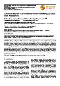
Thus, the fuzzy-molecular inference model is finally expressed in (11). Figure 2 shows the fuzzy-molecular inference model as a block diagram. This model represents a nonlinear inference system for a given crisp input 𝑥 ∈ 𝑋 that follows three steps, that is, fuzzification, fuzzy inference engine, and defuzzification, and obtains the corresponding crisp output 𝑦 ∈ 𝑌, where 𝑌 represents the output. Moreover, fuzzy rules like (9) can also be expressed as a fuzzy matrix that defines a knowledge base of the problem domain. Each block in the FMI-model is detailed in the following subsections. 3.1. Fuzzification. The fuzzy-molecular inference model can be viewed as a block with inputs and outputs. Moreover, let any given system be a single-input-single-output. Then, fuzzification maps any given input variable 𝑥, also known

Mathematical Problems in Engineering

5

Knowledge base

x

y

If ,then Fuzzification

Inference engine

Defuzzification

as a linguistic variable, to a fuzzy value in the range [0, 1]. In particular, this mapping occurs using a fuzzy set 𝐴 and its corresponding membership function 𝜇𝐴 (𝑥), such that (12) holds: (12)

In fact, this linguistic variable is partitioned into 𝑚 different fuzzy sets {𝐴 𝑖 }, for all 𝑖 = 1, . . . , 𝑚. For example, this fuzzy partition can be “low,” “medium,” “high.” Then, the evaluation of a given value of 𝑥 is calculated using the set of membership functions 𝜇𝐴 𝑖 (𝑥), for all 𝑖 = 1, . . . , 𝑚. The shape of all membership functions depends on the purpose of the problem domain. The literature reports different criteria and methods to do so as in [7–9, 11, 23, 24]. 3.2. Fuzzy Inference Engine. Once the crisp value of the input is mapped to a fuzzy subspace as described in Section 3.1, the next step in the fuzzy-molecular inference model is the evaluation of the antecedents in fuzzy rules like (11). In this work, the min function (13) is selected for the 𝑇-norm Δ 𝜇Δ (𝑥1 , . . . , 𝑥𝑘 ) = min {𝜇𝐴 1 (𝑥1 ) , . . . , 𝜇𝐴 𝑘 (𝑥𝑘 )} .

(13)

Finally, the consequent value 𝑦𝑖 is equal to the valuedbehavior 𝜑𝑗 of the 𝑗th CH-molecule of an artificial hydrocarbon network. Thus, the consequent value 𝑦𝑖 can be calculated using fuzzy rules (11) with the min function (13), as shown in (14) 𝑦𝑖 = 𝜑𝑗 (min {𝜇𝐴 1 (𝑥1 ) , . . . , 𝜇𝐴 𝑘 (𝑥𝑘 )}) .

(14)

3.3. Defuzzification. The last step in fuzzy-molecular inference model calculates the crisp value of the output 𝑦 (15) using 𝑛 fuzzy rules, where 𝑦𝑖 is the consequent value and 𝜇Δ𝑖 (𝑥1 , . . . , 𝑥𝑘 ) is the fuzzy evaluation of the antecedents, for 𝑖 = 1, . . . , 𝑛. In particular, (15) is based on the well-known center of gravity [10] 𝑦=

∑ 𝜇Δ𝑖 (𝑥1 , . . . , 𝑥𝑘 ) ⋅ 𝑦𝑖 . ∑ 𝜇Δ𝑖 (𝑥1 , . . . , 𝑥𝑘 )

C = M1 –M2 – ⋅ ⋅ ⋅ − M𝑗 – ⋅ ⋅ ⋅ –M𝑝−1 –M𝑝 = CH3 –CH2 – ⋅ ⋅ ⋅ –CH2 – ⋅ ⋅ ⋅ –CH2 –CH3 .

Figure 2: Block diagram of the fuzzy-molecular inference model.

𝜇𝐴 : 𝑥 󳨃󳨀→ [0, 1] .

that is made of 𝑝 CH-primitive molecules with molecular behavior of the form as in (2). In this work, compound C is restricted to a linear chain of CH-molecules like in (16), where − stands for a covalent bond. Actually, the linear chain is made of 2 CH3 molecules at both extremes and (𝑝−2) CH2 molecules in the inner chain

(15)

As noticed in Section 3.2, the fuzzy-molecular inference model requires a set of CH-molecules. In this case, let AHN be an artificial hydrocarbon network with one compound C

(16)

It is remarkable to say that in the fuzzy-molecular inference model, the AHN is restricted to one univariate compound with one input 𝜇Δ (𝑥1 , . . . , 𝑥𝑘 ) defined as (13) and one output 𝑦𝑖 defined as (14). In case that a multiple-inputs-single-output (MISO) system has to be applied for a particular AHN, consider generalizing (1) as a multivariate function. 3.4. Knowledge Base. Since, the fuzzy-molecular inference model has a generic fuzzy inference engine, proper knowledge of a specific problem domain can be enclosed into the knowledge base (see Figure 2). For instance, this knowledge base is a matrix that summarizes all fuzzy rules of the form as in (11) in the following way. (a) For all input variables 𝑥1 , . . . , 𝑥𝑘 , represent all possible combinations of them using the label of each set in the fuzzy partition of inputs, such that all antecedents in the fuzzy rules will be covered. (b) For each combination (summary of antecedents), assign the corresponding label of molecule M𝑗 that will act when the fuzzy rule is fired. As an example of the knowledge base matrix construction, assume that there is a set of fuzzy rules like (17); thus, the knowledge base matrix for this particular system is shown in Table 1 𝑅1 : If 𝑥1 is 𝐴 1 and 𝑥2 is 𝐵2 , then 𝑦1 is M1 , 𝑅2 : If 𝑥1 is 𝐴 2 and 𝑥2 is 𝐵1 , then 𝑦2 is M1 ,

(17)

𝑅3 : If 𝑥1 is 𝐴 1 and 𝑥2 is 𝐵1 , then 𝑦3 is M2 . 3.5. Properties of the Fuzzy-Molecular Inference Model. The fuzzy-molecular inference model combines interesting properties from both fuzzy logic and artificial hydrocarbon networks. Advantages of the FMI-model are as the following. (i) Fuzzy partitions in the output domain might be seen as linguistic units, for example, “low,” “high.” (ii) Fuzzy partitions have a degree of understanding (parameters are metadata). (iii) Molecular units deal with noise and uncertainties. It is remarkable to say that molecules are excited by consequent values; thus, molecules do not model a given system, but transfer information from a fuzzy subspace to a crisp set. Moreover, molecular units have the property of filtering noise and uncertainties, especially important in realworld control applications, as described in Section 5.

6

Mathematical Problems in Engineering Table 1: Knowledge base of (17).

𝑥1 𝐴1 𝐴2 𝐴1

𝑥2 𝐵2 𝐵1 𝐵1

r(t)

𝑦𝑖 M1 M1 M2

e(t) −

z

Control law

−1

u(t)

y(t)

DC motor

̇ e(t)

4. Design of Fuzzy-Molecular Based Controller for a DC Motor In this section, the design of a velocity controller for a DC motor using the fuzzy-molecular inference model is described. The objective of this fuzzy-molecular controller is to show an example of how to apply the FMI-model as a fuzzy control system. 4.1. Definition of the DC Motor Model. For instance, consider a DC motor that regulates the velocity 𝜔 of its rotor varying the input voltage V. Let 𝐺(𝑠) be the transfer function of a given DC motor expressed in (18) 𝐺 (𝑠) =

𝑠2

1.5 . + 14𝑠 + 40.02

(18)

In order to simulate the performance of the DC motor, a discrete transfer function 𝐺(𝑧) was obtained using (18) and a sample time of 0.01 s. The discrete model of DC motor is shown in (19) 𝐺 (𝑧) =

7.16𝑧 + 6.83 × 10−5 . 𝑧2 − 1.86𝑧 + 0.87

(19)

Finally, if one supposes that DC motor is a causal, linear-time invariant system, then a difference equation of (19) can be expressed as (20), where 𝜔 is the velocity of the rotor, 𝑢 is the input voltage, and 𝑘 is the current sample time 𝜔 [𝑘] = 1.86𝜔 [𝑘 − 1] − 0.87𝜔 [𝑘 − 2] + 7.16 × 10−5 𝑢 [𝑘] + 6.83 × 10−5 𝑢 [𝑘 − 1] . (20) 4.2. Design of Control Law. The following control law is designed to achieve a step response of the DC motor model (20). Assuming the control diagram of Figure 3, the control law has two inputs—the error signal 𝜀(𝑡) and the first ̇ derivative of error signal 𝜀(𝑡)—and one output—the input voltage 𝑢(𝑡). Thus, a fuzzy-molecular PD controller will be designed. Using the fuzzy-molecular inference model described in Section 3, the control law is formed by three blocks: fuzzification, fuzzy inference engine, and defuzzification, as follows.

1 0.8 0.6 0.4 0.2 0 −2

VN

−1.5

VP

NN Z PP

−1

0 0.5 −0.5 Error signal

1

1.5

2

Figure 4: Fuzzy sets of the input error signal.

Membership value

In order to demonstrate the above advantages, an example of the application of the FIM-model in fuzzy control systems is provided in the following section. Then, Section 5 presents a case study that evaluates the performance of the FIM-model in a real application with dynamic uncertainties.

Membership value

Figure 3: Block diagram of the PD control system implemented.

1 0.8 0.6 0.4 0.2 0 −2

VN

−1.5

NN Z PP

−1

0 0.5 1 −0.5 First derivative error signal

VP

1.5

2

Figure 5: Fuzzy sets of the input first derivative error signal.

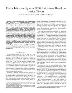
4.2.1. Fuzzification. The two input variables are partitioned into five fuzzy sets: “very negative” (VN), “negative” (NN), “zero” (Z), “positive” (PP), and “very positive” (VP). Figure 4 shows the fuzzy sets of the input variable 𝜀(𝑡), and Figure 5 ̇ It is remarkable shows the fuzzy sets of the input variable 𝜀(𝑡). that parameters in the membership functions were tuned manually, and the input domain was previously normalized. 4.2.2. Fuzzy Inference Engine. The fuzzy inference engine for the fuzzy-molecular PD controller uses fuzzy rules of the form as in (11) with consequent values as in (14). In particular to the application, the implemented knowledge base is summarized in Table 2. Notice that Table 2 reports, for each combination of input values, the fired molecule. For instance, the output signal was partitioned into five CH-molecules M𝑗 , for all 𝑗 = 1, . . . , 5, that represent the action to be held. In particular, the output signal was partitioned into the following molecules: “very negative” (MVN ), “negative” (MNN ), “zero” (MZ ), “positive” (MPP ), and “very positive” (MVP ). 4.2.3. Defuzzification. The input voltage 𝑢(𝑡), the input signal of the plant, is the output variable that defines the last block of the fuzzy-molecular PD controller. In order to calculate the consequent values of fuzzy rules depicted in Section 4.2.2, the five CH-molecules are proposed in Figure 6 and were found using Algorithm 1. Notice that the output variable is

Mathematical Problems in Engineering

7

Table 2: Knowledge base of the fuzzy-molecular PD controller for DC motor. VN MVN MVN MVN MPP MVP

VN NN Z PP VP

−4.55E6 −1.01E15

0

NN MVN MVN MNN MVP MVP 0

𝜀̇ Z MVN MVN MZ MVP MVP

PP MVN MVN MPP MVP MVP

VP MVN MNN MVP MVP MVP

1.13E15 −7.52E7

C

C

C

C

C

4.55E6

0

0

0

7.52E7

𝜎𝑗 +2.41𝐸 − 14 −4.97𝐸 − 16 0.0 −4.43𝐸 − 16 −8.85𝐸 − 17

CH-molecule MVN MNN MZ MPP MVP

1 0

Figure 6: Artificial hydrocarbon network used in the fuzzymolecular PD controller.

Angular velocity

𝜀

Table 3: Adjustment parameters of molecules in the fuzzymolecular PD controller.

0.8 0.6 0.4 0.2 0

finally evaluated using (15), and resultant value is normalized. Finally, the adjustment parameters 𝜎𝑗 of CH-molecules are summarized in Table 3.

0.5

1

1.5 Time (s)

2

2.5

3

Reference FMI

Figure 7: Step response of the fuzzy-molecular PD controller for DC motor. 0.6 0.4 Derivative error signal

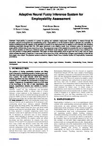
4.3. Results of the Velocity Control for a DC Motor. The fuzzymolecular PD velocity controller for a DC motor described above was implemented and simulated. For instance, the objective of this application is to measure the performance of the system for a step response. The system was subjected to a step function as shown in Figure 7. Results determine that the step response has 17% of maximum overshoot, a rise time of 0.19 s, a settling time of 0.45 s, and a maximum error of 0.002 in steady state. In order to measure the stability of the fuzzy-molecular PD controller, a phase diagram was obtained from the step response. Figure 8 shows the phase diagram of error signal versus derivative of error signal. As it can be seen in Figure 8, the fuzzy-molecular PD controller reaches a steady state near to the zero input state vector of the controller. Then, the step was implemented with a reference signal varying in the range from −2 to 2 ×1000 rpm. After 10 seconds with a sample time of 0.01 s, the step response is depicted in Figure 9, where the light line represents the reference signal and the strong line represents the actual value of angular velocity of the rotor in the DC motor. As shown in Figure 9, the fuzzy-molecular PD controller has an excellent performance. From the results obtained so far, it can be seen that the performance of the fuzzy-molecular PD controller has a very good quality (see Figure 8). The maximum overshoot, the settling time, and the maximum error in steady state correspond to the performance of a PD controller as reported in the literature of control theory [25]. On the other hand, the fuzzy-molecular PD controller was easily obtained. In this case, fuzzification was done via fuzzy sets tuned manually; however, there are other ways to find the optimal values of parameters in membership functions (see [7–9, 11, 23, 24]). In addition, defuzzification

0

0.2 0 −0.2 −0.4 −0.6 −0.8 −1 −0.2

0

0.2

0.4 Error signal

0.6

0.8

1

Figure 8: Phase diagram derivative error signal versus error signal in the step response of the fuzzy-molecular PD controller for DC motor.

was implemented with an artificial hydrocarbon network that depends on hydrogen and adjustment parameters that can be easily found using Algorithm 1.

5. Case Study: Fuzzy-Molecular Based Position Controller for a DC Motor In this section, the design of a position controller for a DC motor using the fuzzy-molecular inference model is described. The objective of this case study is to improve type2 fuzzy control systems using the fuzzy-molecular inference model.

8

Mathematical Problems in Engineering 2.5

r(t)

Angular velocity

2

e(t) −

z

1.5

Control law

̇ y(t) −1

u(t)

y(t)

DC motor

1

Figure 11: Block diagram of the position control system implemented.

0.5

−0.5

0

1

2

3

4

5 6 Time (s)

7

8

9

10

Reference FMI

Figure 9: Step response of the fuzzy-molecular PD controller for DC motor. Trainer module (DC motor)

Computer (monitoring)

Figure 10: Overall system of the case study showing the trainer hardware module, the NI CompactRIO host, and the LabVIEW client for monitoring the system.

5.1. Description of the Hardware. The following case study was implemented on a trainer hardware module. It is prepared for sending reference signals (i.e., from a knob) and feedback signals (i.e., the current position of a DC motor) to a host in which a control law is running. The correction signal computed is sent back to the trainer module in order to feed a DC motor. In particular to this case study, a NI CompactRIO reconfigurable and embedded system based on field programmable gate arrays (FPGA) is used as the host. Figure 10 shows the overall system. In addition, LabVIEW software is used for programming the control law on the NI CompactRIO and for monitoring the performance of the fuzzy-molecular control system. On one hand, both the reference signal 𝑟(𝑡) that comes from a knob and the position signal 𝑦(𝑡) are in the voltage range [0.0, 5.0] V, where 0.0 V represents an angle of 0∘ and 5.0 V represents an angle of 180∘ . On the other hand, the correction signal 𝑢(𝑡) is the input voltage of the DC motor in the range [0.0, 5.0] V, where 0.0 V represents the maximum angular velocity of the motor to rotate counterclockwise,

1 0.8 0.6 0.4 0.2 0 −1

N

P

Z

0.2 −0.8 −0.6 −0.4 −0.2 0 Error signal

0.4

0.6

0.8

1

Figure 12: Fuzzy sets of the input error signal. Solid line: primary membership function. Dashed line: secondary membership function.

Membership value

Host (with FPGA)

Membership value

0

1 0.8 0.6 0.4 0.2 0 −1

N

Z

P

0.2 0.4 0.6 −0.8 −0.6 −0.4 −0.2 0 First derivative position signal

0.8

1

Figure 13: Fuzzy sets of the input first derivative position signal. Solid line: primary membership function. Dashed line: secondary membership function.

5.0 V represents the maximum angular velocity of the motor to rotate clockwise, and 2.5 V means no rotation. It is remarkable to say that the position of the DC motor increases in counterclockwise direction and decreases in clockwise direction. 5.2. Design of Control Law. The following control law is designed to achieve a reference tracking response of the DC motor in the trainer model. Assuming the control diagram of Figure 11, the control law has two inputs—the error signal ̇ 𝜀(𝑡) and the first derivative of the position signal 𝑦(𝑡)—and one output—the input voltage 𝑢(𝑡). Thus, a fuzzy-molecular PD controller will be designed. Using the fuzzy-molecular inference model described in Section 3, the control law is designed as follows. 5.2.1. Fuzzification. The two input variables are partitioned into three type-2 fuzzy sets: “negative” (N), “zero” (Z), and “positive” (P). Figure 12 shows the fuzzy sets for input ̇ 𝜀(𝑡), and Figure 13 shows the fuzzy sets for input 𝑦(𝑡). It is remarkable to say that parameters in the membership functions were tuned manually.

Mathematical Problems in Engineering

9

Table 4: Knowledge base of the fuzzy-molecular position controller for the DC motor in the trainer module. N MCW MCW MCCW

N Z P

−0.8

−0.4

0

−0.4

C

C

C

0.4

0

0.4

P MCW MCCW MCCW

−0.8

Figure 14: Artificial hydrocarbon network used in the fuzzymolecular position controller.

As shown in Figures 12 and 13, type-2 fuzzy sets are determined by primary membership function 𝜇𝐴𝑈(𝑥) but also considers an additional value of uncertainty: the secondary membership function 𝜇𝐴𝐿 (𝑥). The region inside these two membership functions is known as the footprint of uncertainty FOU [10, 14] as expressed in (21) FOU (𝐴) = ⋃ 𝑥∈𝑋

(𝜇𝐴𝐿 (𝑥) , 𝜇𝐴𝑈 (𝑥)) .

𝜎𝑗 −1.0 0.0 1.0

CH-molecule MCW MH MCCW

Membership value

𝜀

𝑦̇ Z MCW MH MCCW

Table 5: Adjustment parameters of molecules in Figure 6.

CW

1

H

CCW

0.8 0.6 0.4 0.2 0

0

0.5

1

1.5

2 2.5 3 3.5 Correction signal

4

4.5

5

Figure 15: Fuzzy sets of the output correction signal. Solid line: primary membership function. Dashed line: secondary membership function.

generates a type reduction [26] of the form as in (22), where 𝑦 is the crisp output value 𝑢(𝑡) 𝑦=

𝑦𝐿 + 𝑦𝑈 . 2

(22)

(21)

Then, two membership values (from primary and secondary functions) are computed for one input value. Moreover, if the secondary membership function coincides with the primary membership function, type-2 is reduced to an equivalent type-1 fuzzy system. 5.2.2. Fuzzy Inference Engine. The fuzzy inference engine for the fuzzy-molecular position controller uses fuzzy rules of the form as in (11) of both primary and secondary membership values (𝜇𝐴𝐿 (𝑥), 𝜇𝐴𝑈(𝑥)). Consequent values 𝑦𝐿 and 𝑦𝑈 are similarly obtained as (15) for both primary and secondary membership values, respectively. The resultant knowledge base is summarized in Table 4. As noted in Table 4, the output signal was partitioned into three CH-molecules M𝑗 , for all 𝑗 = 1, . . . , 3, that represent the action to be held. In particular, the output signal was partitioned into the following molecules: “clockwise” (MCW ), “halt” (MH ), and “counterclockwise” (MCCW ). 5.2.3. Defuzzification. In order to calculate the consequent values of fuzzy rules depicted in Table 4, the three CHmolecules are proposed in Figure 14 and were found using Algorithm 1. The adjustment parameters 𝜎𝑗 of CH-molecules are summarized in Table 5. In this case study, the Nie-Tan method [26] is used for computing the final value of the output variable 𝑢(𝑡) for a type-2 fuzzy system because of its simplicity of computation. Other methods like Karnik-Mendel, Greenfield-Chiclana, or Wu-Mendel might be used [10, 12–14, 26]. The method

6. Results and Discussion In order to demonstrate that the fuzzy-molecular inference model for fuzzy control systems can be used as an alternative of type-2 fuzzy control systems, two experiments were done. The first experiment considers a type-1 fuzzy controller system and the second experiment considers a type-2 fuzzy controller system. In both cases, the FIMmodel based fuzzy control system designed in Section 5 is compared with a Mamdani’s fuzzy controller system using the same parameters. The output variable was partitioned for the Mamdani’s fuzzy controller system into three type-2 fuzzy sets: “clockwise” (CW), “halt” (H), and “counterclockwise” (CCW). Figure 15 shows this partition for the output variable 𝑢(𝑡). 6.1. Performance of the Type-1 Fuzzy-Molecular Controller. For this experiment, the fuzzy-molecular position controller for a DC motor described in Section 5 was reduced to a type1 fuzzy system by only considering the primary membership functions in the fuzzification step, as well as in the Mamdani’s fuzzy controller. The system was subjected to a step function without noise as shown in Figure 16. Results of the FMI controller determine that it had a step response of 0% of maximum overshoot, a rise time of 1.0 s, and a maximum error of 2.5∘ in steady state. On the other hand, the system was subjected to a step function with 35% of noise as shown in Figure 17. Results of the FMI controller reports a 0% of maximum overshooting, a rise time of 1.1 s, and a maximum error of 5.8∘ in steady state measured from position 180∘ . For contrasting, Table 6

Position (∘ )

10

Mathematical Problems in Engineering 180 160 140 120 100 80 60 40 20 0

Table 6: Experimental results of type-1 fuzzy controllers.

0

1

2

3 Time (s)

4

5

6

Reference FMI Mamdani

Fuzzy controller Noise (%) Rise time (s) Step Response FIM 0.0 1.0 Mamdani 0.0 2.0 FIM 35.0 1.1 Mamdani 35.0 2.5 Ramp response FIM 0.0 — Mamdani 0.0 — FIM 35.0 — Mamdani 35.0 —

Figure 16: Step response without noise of FMI and Mamdani type-1 fuzzy controllers.

Steady-state error (∘ ) 2.5 4.7 5.8 5.5 3.6 6.7 11.0 12.3

180

Position (∘ )

150

Position (∘ )

200 180 150 100

100 50 0

50

0

1

0 0

1

2

3 Time (s)

4

5

6

Reference FMI Mamdani

Figure 17: Step response with 35% noise of FMI and Mamdani type1 fuzzy controllers.

summarizes the overall results of the FMI and Mamdani fuzzy controllers. Notice in Figure 16 that the response of the FMI controller is 50% faster than the response of the Mamdani controller and has a less value of maximum error in steady state than then Mamdani controller. In comparison, Figure 17 shows that both fuzzy controllers are well stable as measured (5.8∘ and 5.5∘ of maximum error in steady state). However, FMI controller is still faster (1.1 s of rise time) than the response of the Mamdani controller (2.5 s of rise time). As noted, FMI controller has a better response for dynamic uncertainties than the Mamdani controller. Also, the system was subjected to a ramp function without noise as shown in Figure 18. Results determine that the FIM controller has a maximum error of 3.6∘ in steady state while the Mamdani controller has 6.7∘ . On the other hand, the system was subjected to a ramp function with 35% of noise as shown in Figure 19. The FMI controller reports 11.0∘ of maximum error in steady state, and the Mamdani controller reports 12.3∘ . Also, Table 6 summarizes the overall results of this experiment with respect to the response of FMI and Mamdani fuzzy controllers.

2

3

4 Time (s)

5

6

7

Reference FMI Mamdani

Figure 18: Ramp response without noise of FMI and Mamdani type1 fuzzy controllers.

It is evident from Table 6 that both fuzzy controllers decrease their performance in presence of noise. However, the FIM controller can track the reference signal better than the Mamdani controller, as shown in the steady-state error. In addition, note that the FMI controller is slightly faster than the Mamdani controller. 6.2. Performance of the Type-2 Fuzzy-Molecular Controller. For this experiment, the type-2 fuzzy-molecular position controller for a DC motor described in Section 5 was implemented as well as the type-2 Mamdani controller. Again, the system was subjected to a step function with 35% noise and without it as shown in Figures 20 and 21, respectively. The same process was done with a ramp function, and the responses of both controllers are shown in Figures 22 and 23, respectively. The overall results are summarized in Table 7. As noted from Tables 6 and 7, the step responses of both FIM and Mamdani type-2 fuzzy controllers remain similar to type-1 controllers, as expected. Thus, type-1 and type-2 FIM fuzzy controllers are slightly equivalent with or without perturbations. From Figures 22 and 23, it can be seen that the response of type-2 fuzzy controllers slightly better than type-1 controllers, as expected [10, 12–14, 26]. From the point of view of ramp

Mathematical Problems in Engineering

11

Position (∘ )

Position (∘ )

180 150 100 50

200 180 150 100 50 0

0 0

1

2

3

4 Time (s)

5

6

0

7

Figure 19: Ramp response with 35% noise of FMI and Mamdani type-1 fuzzy controllers.

3 Time (s)

4

5

6

Figure 21: Step response with 35% noise of FMI and Mamdani type2 fuzzy controllers.

180 150 Position (∘ )

Position (∘ )

2

Reference FMI Mamdani

Reference FMI Mamdani

180 160 140 120 100 80 60 40 20 0

1

100 50 0

0

1

2

3 Time (s)

4

5

6

Reference FMI Mamdani

0

1

2

3

4 Time (s)

5

6

7

Reference FIM Mamdani

Figure 20: Step response without noise of FMI and Mamdani type-2 fuzzy controllers.

Figure 22: Ramp response without noise of FMI and Mamdani type-2 fuzzy controllers.

response, the FIM controller presents similar performance to the Mamdani controller without noise (3.8∘ and 3.7∘ maximum steady-state errors, resp.). Again, both controllers present the same tendency when they are exposed to noise, and in comparison with type-1 controllers, type-2 fuzzy controllers act slightly better as found in Tables 6 and 7 (FIM: 17.2% better, Mamdani: 1.7% better).

models like Takagi-Sugeno inference systems or Mamdani’s fuzzy control systems [7–9, 11]. Thus, Table 8 presents a comparative chart of the FMI-model, Takagi-Sugeno’s model, and Mamdani’s model. From Table 8, defuzzification process in each fuzzy inference model is different. As FMI-model uses artificial hydrocarbon networks, each molecule represents a linguistic partition of the output variable. In the above results, simple CH-molecules were implemented, but either complex molecules can be used. Thus, defuzzification can have complex nonlinear mappings in the FMI-model. In contrast, Takagi-Sugeno’s model uses polynomial functions, and Mamdani’s model represents linguistic partitions with membership functions associated with fuzzy sets. Parameters inside artificial hydrocarbon networks are hydrogen and adjustment values, polynomial coefficients for Takagi-Sugeno’s model, and parameters of membership functions in Mamdani’s model. In addition, molecules in FMI-model make a mapping from membership or truth-values to output values also dealing with uncertainties. This is remarkable because TakagiSugeno’s model maps from input values to output values,

6.3. Discussion of FIM-Models. On one hand, from the above results, fuzzy-molecular inference models can achieve fuzzy control applications. Moreover, these FIM-model based controllers can be used as an alternative of type-2 fuzzy control systems. This statement comes from the evaluation and comparison of step and ramp responses between the FIM-controller designed in Section 5 and the Mamdani fuzzy controller; both models subjected to static and dynamic uncertainties. In this case study, a Mamdani’s fuzzy control system was used because it is the fuzzy inference system most implemented in industry as reported in the literature [10, 14]. On the other hand, it is important to distinguish the fuzzy-molecular inference model from other fuzzy inference

Mathematical Problems in Engineering

Position (∘ )

12

180 150 100 50 0 0

1

2

3

4 Time (s)

5

6

7

Reference FIM Mamdani

Figure 23: Ramp response with 35% noise of FMI and Mamdani type-2 fuzzy controllers. Table 7: Experimental results of type-2 fuzzy controllers. Fuzzy controller Noise (%) Rise time (s) Step Response FIM 0.0 1.0 Mamdani 0.0 2.4 FIM 35.0 1.0 Mamdani 35.0 2.6 Ramp response FIM 0.0 — Mamdani 0.0 — FIM 35.0 — Mamdani 35.0 —

Steady-state error (∘ ) 2.5 4.7 5.0 5.5 3.8 3.7 9.1 12.1

Table 8: Comparative chart of different fuzzy inference models. FMI-model Defuzzification AHNs

Takagi-Sugeno

Mamdani

Polynomial functions

Membership functions

Hydrogen values Coefficients Adjustment values Membership Mappings in Input values to values to output defuzzification output values values Definition of parameters

Parameters of membership functions Membership values to output values

and using fuzzy inference values linearly acts on the final output value. At last, Mamdani’s model makes a mapping from membership values to output values. In fact, the fuzzymolecular inference model combines linguistic partitions of output variables with molecular structures.

7. Conclusions In this paper, a new fuzzy algorithm based on artificial hydrocarbon networks called fuzzy-molecular inference model (FMI-model) was proposed, taking advantage of the power of molecular units of information. In this approach, molecules

of artificial hydrocarbon networks are implemented as fuzzy partitions in the output domain. Since the FMI-model is based on AHNs, properties of molecules are inherited. Two characteristics of the proposed fuzzy-molecular inference model are both interpretation of linguistic molecules and partial understanding of fuzzy partitions via metaparameters in AHNs. In that way, the novel fuzzy algorithm treats molecules as fuzzy partitions of the output variable, transferring information from a fuzzy subspace to a crisp set, allowing to set the number of fuzzy partitions linguistically, but also these molecules are characterized by hydrogen values that can be referred to as meta-data information, giving the opportunity to partially understand the molecular behavior. Moreover, the proposed fuzzy-molecular inference model has some advantages in comparison with other fuzzy inference systems. For instance, FMI-model occupies parameters with metadata information in comparison with Mamdani’s inference system in which parameters associated with membership functions do not reveal important information of the fuzzy partition. If parameters are meta-data information, it is easier to tune fuzzy partitions because both experts and real data information coming from the system can be combined into a single unit, no matter how complex the mapping is. In addition, since FMI-model does not model a given system like Takagi-Sugeno’s inference system, it preserves a more natural way of defuzzification from a fuzzy subspace to a crisp set. Finally, since molecules in artificial hydrocarbon networks can filter information [18, 19], the fuzzy-molecular inference model also shares this property allowing to deal with uncertain data. Thus, the proposed fuzzy-molecular inference model has three steps: fuzzification, fuzzy inference engine, and defuzzification. Specially, molecules are mappings from implication values to output variables. In addition, in this work, a linear chain of CH-primitive molecules was used, but the FMI-model allows complex molecules associated with each fuzzy rule handling complex nonlinear mappings from fuzzy subspaces to crisp sets. On the other hand, the proposed model was applied to control the angular velocity of a simulated DC motor in which the results confirm that the FMI-model can be used in control applications. Furthermore, a case study was presented in which the FMI-model was used for controlling the position of a real DC motor. Experimental results demonstrate that fuzzy-molecular based control systems can deal with uncertainties as type-2 fuzzy control systems do. Then, it suggests that FMI-based controllers can be used as an alternative of type-2 fuzzy control systems. In practical applications where hardware restricts the operational computations or memory storage, FMI-based controllers can be implemented because of its simplicity. Future research considers the design of training procedures for optimality in molecules at the defuzzification stage of FMI-models. In addition, since artificial hydrocarbon networks are considered under the class of learning algorithms, the usage of molecular units in FMI-models might be applied for online adaptation (learning and evolution) of the overall fuzzy control system to improve its performance.

Mathematical Problems in Engineering

Acknowledgments This work was supported by a scholarship award from Tecnol´ogico de Monterrey, Campus Ciudad de M´exico and a scholarship for living expenses from CONACYT.

References [1] L. Xia and Y. Xiuju, “The application of adaptive fuzzy inference model in the nonlinear dynamic system identificatio,” in Proceedings of the 2nd International Conference on Intelligent Computing Technology and Automation (ICICTA ’09), pp. 814– 817, October 2009. [2] H. Seki, “Type-2 fuzzy functional SIRMs connected inference model,” in Proceedings of the 6th International Conference on Soft Computing and Intelligent Systems and 13th International Symposium on Advanced Intelligent Systems, pp. 1615–11620, 2012. [3] K.-E. Ko and K.-B. Sim, “An EEG signals classification system using optimized adaptive neuro-fuzzy inference model based on harmony search algorithm,” in Proceedings of the 11th International Conference on Control, Automation and Systems (ICCAS ’11), pp. 1457–1461, October 2011. [4] Y.-P. Huang, T.-W. Chang, and F.-E. Sandnes, “Improving image retrieval efficiency using a fuzzy inference model and genetic algorithm,” in Proceedings of the Annual Meeting of the North American Fuzzy Information Processing Society, pp. 361–366, June 2005. [5] C. Gong and C. Han, “Robust 𝐻∞ control of uncertain TS fuzzy time-delay system: a delay decomposition approach,” Mathematical Problems in Engineering, vol. 2013, Article ID 345601, 10 pages, 2013. [6] W. Huang and S.-K. Oh, “Identification of fuzzy inference systems by means of a multiobjective opposition-based space search algorithm,” Mathematical Problems in Engineering, vol. 2013, Article ID 725017, 13 pages, 2013. [7] T. Takagi and M. Sugeno, “Fuzzy identification of systems and its applications to modeling and control,” IEEE Transactions on Systems, Man and Cybernetics, vol. 15, no. 1, pp. 116–132, 1985. [8] E. H. Mamdani, “Application of fuzzy algorithms for control of simple dynamic plant,” IEEE Proceedings of the Institution of Electrical Engineers, vol. 121, no. 12, pp. 1585–1588, 1974. [9] Y. Tsukamoto, “An approach to fuzzy reasoning method,” in Advances in Fuzzy Set Theory and Applications, M. Gupta, R. Ragade, and R. Yager, Eds., pp. 137–149, North-Holland, Amsterdam, The Netherlands, 1979. [10] I. Iancu, “A mamdani type fuzzy logic controller,” in Fuzzy Logic: Controls, Concepts, Theories and Applications, pp. 325– 350, InTech, 2012. [11] J.-S. R. Jang and C.-T. Sun, “Neuro-fuzzy modeling and control,” Proceedings of the IEEE, vol. 83, no. 3, pp. 378–406, 1995. [12] O. Linda and M. Manic, “Comparative analysis of Type-1 and Type-2 fuzzy control in context of learning behaviors for mobile robotics,” in Proceedings of the 36th Annual Conference of the IEEE Industrial Electronics Society (IECON ’10), pp. 1092–1098, November 2010. [13] S. Musikasuwan and J. M. Garibaldi, “On relationships between primary membership functions and output uncertainties in interval type-2 and non-stationary fuzzy sets,” in Proceedings of the IEEE International Conference on Fuzzy Systems, pp. 1433– 1440, July 2006.

13 [14] J. M. Mendel and R. I. B. John, “Type-2 fuzzy sets made simple,” IEEE Transactions on Fuzzy Systems, vol. 10, no. 2, pp. 117–127, 2002. [15] H. Zhang and D. Liu, Fuzzy Modeling and Fuzzy Control, Springer, Boston, Mass, USA, 2006. [16] H. Ponce and P. Ponce, “Artificial organic networks,” in Proceedings of the IEEE Electronics, Robotics and Automotive Mechanics Conference (CERMA ’11), pp. 29–34, November 2011. [17] H. Ponce and P. Ponce, “Artificial hydrocarbon networks,” in Proceedings of the 9th International Conference on Innovation and Technological Development (CIINDET ’11), pp. 614–618, 2011. [18] H. Ponce, P. Ponce, and A. Molina, “A novel adaptive filtering for audio signals using artificial hydrocarbon networks,” in Proceedings of the 9th International Conference on Electrical Engineering, Computing Science and Automation Control, pp. 277–282, 2012. [19] H. Ponce and P. Ponce, “Artificial hydrocarbon networks: a new algorithm bio-inspired on organic chemistry,” International Journal of Artificial Intelligence and Computational Research, vol. 4, no. 1, pp. 39–51, 2012. [20] H. Ponce, P. Ponce, and A. Molina, “A new training algorithm for artificial hydrocarbon networks using an energy model of covalent bonds,” in Proceedings of the IFAC Conference on Manufacturing Modelling, Management and Control, 2013. [21] H. Ponce, P. Ponce, and A. Molina, “Artificial hydrocarbon networks: a bio-inspired computational algorithm for modeling problems,” Tech. Rep., Graduate School of Engineering, Tecnol´ogico de Monterrey, Campus Ciudad de M´exico, Mexico City, Mexico, 2013. [22] H. Ponce and P. Ponce, “A Novel Approach of Artificial Hydrocarbon Networks on Adaptive Noise Filtering for Audio Signals,” Tech. Rep., Graduate School of Engineering, Tecnol´ogico de Monterrey, Campus Ciudad de M´exico, Mexico City, Mexico, 2013. [23] L. M. de Campos and S. Moral, “Learning rules for a fuzzy inference model,” Fuzzy Sets and Systems, vol. 59, no. 3, pp. 247– 257, 1993. [24] Y.-P. Huang, S.-H. Yu, and M.-S. Horng, “An efficient tuning method for designing a fuzzy inference model,” in Proceedings of the IEEE International Conference on Systems, Man and Cybernetics, pp. 1–6, October 2001. [25] K. Ogata, Modern Control Engineering, Prentice Hall, Englewood Cliffs, NJ, USA, 2010. [26] M. Nie and W. W. Tan, “Towards an efficient type-reduction method for interval type-2 fuzzy logic systems,” in Proceedings of the IEEE International Conference on Fuzzy Systems, pp. 1425– 1432, June 2008.

Advances in

Operations Research Hindawi Publishing Corporation http://www.hindawi.com

Volume 2014

Advances in

Decision Sciences Hindawi Publishing Corporation http://www.hindawi.com

Volume 2014

Journal of

Applied Mathematics

Algebra

Hindawi Publishing Corporation http://www.hindawi.com

Hindawi Publishing Corporation http://www.hindawi.com

Volume 2014

Journal of

Probability and Statistics Volume 2014

The Scientific World Journal Hindawi Publishing Corporation http://www.hindawi.com

Hindawi Publishing Corporation http://www.hindawi.com

Volume 2014

International Journal of

Differential Equations Hindawi Publishing Corporation http://www.hindawi.com

Volume 2014

Volume 2014

Submit your manuscripts at http://www.hindawi.com International Journal of

Advances in

Combinatorics Hindawi Publishing Corporation http://www.hindawi.com

Mathematical Physics Hindawi Publishing Corporation http://www.hindawi.com

Volume 2014

Journal of

Complex Analysis Hindawi Publishing Corporation http://www.hindawi.com

Volume 2014

International Journal of Mathematics and Mathematical Sciences

Mathematical Problems in Engineering

Journal of

Mathematics Hindawi Publishing Corporation http://www.hindawi.com

Volume 2014

Hindawi Publishing Corporation http://www.hindawi.com

Volume 2014

Volume 2014

Hindawi Publishing Corporation http://www.hindawi.com

Volume 2014

Discrete Mathematics

Journal of

Volume 2014

Hindawi Publishing Corporation http://www.hindawi.com

Discrete Dynamics in Nature and Society

Journal of

Function Spaces Hindawi Publishing Corporation http://www.hindawi.com

Abstract and Applied Analysis

Volume 2014

Hindawi Publishing Corporation http://www.hindawi.com

Volume 2014

Hindawi Publishing Corporation http://www.hindawi.com

Volume 2014

International Journal of

Journal of

Stochastic Analysis

Optimization

Hindawi Publishing Corporation http://www.hindawi.com

Hindawi Publishing Corporation http://www.hindawi.com

Volume 2014

Volume 2014