Artificial Intelligence Techniques for Flood Risk Management in Urban ...

Artificial Intelligence Techniques for Flood Risk Management in Urban Environments Submitted by

William Keith Paul Sayers To the University of Exeter as a Thesis for the degree of Doctor of Engineering in Water Engineering

November 2015

This thesis is available for Library use on the understanding that it is copyright material and that no quotation from the thesis may be published without proper acknowledgement. I certify that all material in this thesis which is not my own work has been identified and that no material has previously been submitted and approved for the award of a degree by this or any other university. …………………………….

1

Abstract

Abstract Flooding is an important concern for the UK, as evidenced by the many extreme flooding events in the last decade. Improved flood risk intervention strategies are therefore highly desirable. The application of hydroinformatics tools, and optimisation algorithms in particular, which could provide guidance towards improved intervention strategies, is hindered by the necessity of performing flood modelling in the process of evaluating solutions. Flood modelling is a computationally demanding task; reducing its impact upon the optimisation process would therefore be a significant achievement and of considerable benefit to this research area. In this thesis sophisticated multi-objective optimisation algorithms have been utilised in combination with cutting-edge flood-risk assessment models to identify least-cost and most-benefit flood risk interventions that can be made on a drainage network. Software analysis and optimisation has improved the flood risk model performance. Additionally, artificial neural networks used as feature detectors have been employed as part of a novel development of an optimisation algorithm. This has alleviated the computational time-demands caused by using extremely complex models. The results from testing indicate that the developed algorithm with feature detectors outperforms (given limited computational resources available) a base multi-objective genetic algorithm. It does so in terms of both dominated hypervolume and a modified convergence metric, at each iteration. This indicates both that a shorter run of the algorithm produces a more optimal result than a similar length run of a chosen base algorithm, and also that a full run to complete convergence takes fewer iterations (and therefore less time) with the new algorithm. 2

Acknowledgements

Acknowledgements First, I would like to thank my academic supervisors, Dragan Savic and Zoran Kapelan, and my industrial supervisor, Richard Kellagher, for their help, guidance, and hard work on my behalf throughout the course of my EngD. I could not have achieved this without their assistance. I would also like to thank my colleagues at HR Wallingford, and particularly the members of the floods and water groups. The floods group welcomed me into their team and included me as one of their own, and the water group provided a large amount of essential advice and assistance. Additionally, I am very grateful to the members of staff and fellow researchers at the University of Exeter and particularly the Centre for Water Systems, who have aided me and helped me to get to where I am today. I wish to thank the STREAM-IDC programme and the EPSRC for making this project possible, as well as all the events and courses they have arranged and/or funded as part of my EngD experience. Finally, I wish to thank my parents, family and friends for their support and encouragement, and particularly my partner Louise for her love, support, encouragement and faith in me throughout this project.

3

List of Tables

Table of Contents Abstract ............................................................................................................... 2 Acknowledgements ............................................................................................. 3 Table of Contents ................................................................................................ 4 List of Tables ..................................................................................................... 12 List of Figures .................................................................................................... 14 List of Abbreviations .......................................................................................... 20 List of Terms ...................................................................................................... 24 1. Introduction ................................................................................................ 27 1.1 General Introduction ................................................................................ 27 1.2 Aims and Objectives of Research ............................................................ 30 1.3 Structure of Thesis ................................................................................... 31 2. Literature Review ....................................................................................... 34 2.1 Introduction .............................................................................................. 34 2.2 Flood Risk Management .......................................................................... 35 2.2.1 Introduction ....................................................................................... 35 2.2.2 Urban Flood Risk Analysis ................................................................ 37

4

List of Tables 2.2.3 Flood Risk Management Summary ................................................... 40 2.3 Optimisation Algorithms ........................................................................... 40 2.3.1 Introduction ....................................................................................... 40 2.3.2 Genetic Algorithms ............................................................................ 41 2.3.3 Simulated Annealing ......................................................................... 44 2.3.4 Ant-Colony Optimisation ................................................................... 45 2.3.5 Multi-Objective Optimisation ............................................................. 46 2.3.6 Multi-Objective Evolutionary Algorithms ............................................ 48 2.3.7 Multi-Objective Simulated Annealing ................................................ 51 2.3.8 Multi-Objective Ant-Colony Optimisation ........................................... 51 2.3.9 Optimisation Algorithms Summary .................................................... 52 2.4 Machine Learning .................................................................................... 52 2.4.1 Introduction ....................................................................................... 52 2.4.2 Artificial Neural Networks .................................................................. 54 2.4.3 Bayesian Belief Networks ................................................................. 57 2.4.4 Machine Learning Techniques Summary .......................................... 59 2.5 Multi-Objective Optimisation with Machine Learning ............................... 59

5

List of Tables 2.5.1 Introduction ....................................................................................... 59 2.5.2 Multi-Objective Genetic Algorithm with Adaptive Neural Networks (MOGA-ANN) ............................................................................................. 61 2.5.3 LEMMO ............................................................................................. 62 2.6 Chapter Summary .................................................................................... 64 3. Urban Flood Risk Assessment ................................................................... 67 3.1 Introduction .............................................................................................. 67 3.2 Risk-based Approach .............................................................................. 68 3.3 Flood Risk Analysis Toolset ..................................................................... 68 3.4 Risk Assessment Framework .................................................................. 70 3.4.1 Design Storm Risk Assessment ........................................................ 71 3.5 Risk Assessment Framework Software Components .............................. 75 3.5.1 Component Object Model Interface Module ...................................... 75 3.5.2 Infoworks Collection Systems Drainage Model ................................. 76 3.5.3 Rapid Flood Spreading Model Module .............................................. 76 3.5.4 Depth-Damage Model Module .......................................................... 76 3.6 Software Implementation Issues .............................................................. 77 3.7 Chapter Summary .................................................................................... 78 6

List of Tables 4. Optimisation for Urban Flood Risk Management ....................................... 79 4.1 Introduction .............................................................................................. 79 4.2 Development of the Costing Model .......................................................... 80 4.3 Improvements to EAD Calculation Tool Set ............................................ 82 4.3.1 Identifying Reduced Rainfall Dataset ................................................ 82 4.3.2 SAM-UMC Modifications ................................................................... 95 4.4 Optimisation Solution ............................................................................... 97 4.4.1 Development Language and Framework .......................................... 98 4.4.2 Optimisation Specific Performance Enhancements .......................... 99 4.4.3 Pipe Modelling for Optimisation ........................................................ 99 4.4.4 Storage Modelling for Optimisation ................................................. 102 4.4.5 Orifice Modelling for Optimisation ................................................... 103 4.4.6 Cost Groups .................................................................................... 103 4.4.7 NSGA-II ........................................................................................... 104 4.4.8 NSGA-II and Machine Learning ...................................................... 106 4.5 Optimisation Assessment ...................................................................... 114 4.5.1 Introduction ..................................................................................... 114

7

List of Tables 4.5.2 Optimisation Set Up ........................................................................ 114 4.5.3 Estimating Pareto Front Accuracy ................................................... 116 4.5.4 Diversity Metric ................................................................................ 117 4.5.5 Convergence Metric ........................................................................ 118 4.5.6 Dominated Hypervolume Metric ...................................................... 122 4.6 Chapter Summary .................................................................................. 123 5. Water Distribution System Test-Cases .................................................... 125 5.1 Introduction ............................................................................................ 125 5.2 Selection of Tests .................................................................................. 125 5.3 Objective Function Formulations ........................................................... 129 5.4 Testing Conditions ................................................................................. 130 5.5 Testing of NSGA-II Base ....................................................................... 132 5.6 Meta-model Evaluation .......................................................................... 132 5.7 Accuracy of Generated Pareto Fronts ................................................... 136 5.7.1 NSGA-II Base Algorithm ................................................................. 137 5.7.2 NSGA-II with LEMMO and Initial ANN Structure ............................. 147 5.7.3 NSGA-II with LEMMO and Final ANN Structure ............................. 156

8

List of Tables 5.7.4 Analysis of Results .......................................................................... 166 5.8 Chapter Summary .................................................................................. 180 6. Case Study: Dalmarnock Catchment ....................................................... 182 6.1 Introduction ............................................................................................ 182 6.2 Dalmarnock Catchment Description ...................................................... 182 6.2.1 Original Dalmarnock Model ............................................................. 182 6.2.2 Testing Dalmarnock Model ............................................................. 183 6.3 Allowed Decision Variable Values ......................................................... 185 6.4 Mutation Operator for Dalmarnock ........................................................ 186 6.5 Optimisation Testing Introduction .......................................................... 187 6.6 Reduced Data-set Identification ............................................................. 190 6.7 NSGA-II and LEMMO Optimisation ....................................................... 191 6.7.1 Basic Run Parameters .................................................................... 191 6.7.2 Optimisation Results ....................................................................... 192 6.8 Dalmarnock Optimisation Solution Analysis .......................................... 200 6.9 Chapter Summary .................................................................................. 206 7. Summary and Conclusions ...................................................................... 207

9

List of Tables 7.1 Summary ............................................................................................... 207 7.2 Novel Contributions ............................................................................... 212 7.3 Conclusions ........................................................................................... 214 7.4 Recommendations for Future Work ....................................................... 216 Appendices ...................................................................................................... 218 Appendix I – Software Diagrams ................................................................. 218 NSGA2CS Class Diagram ....................................................................... 219 ADAPTController Class Diagram ............................................................. 220 ADAPT User Interface Class Diagram ..................................................... 221 Appendix II – BIN Data Tables .................................................................... 222 NSGA-II Base Algorithm .......................................................................... 223 NSGA-II with LEMMO and Initial ANN Structure ...................................... 226 NSGA-II with LEMMO and Final ANN Structure ...................................... 228 NSGA-II Base Algorithm Analysis Metric Results .................................... 231 NSGA-II with LEMMO and Initial ANN Structure Analysis Metric Results 238 NSGA-II with LEMMO and Final ANN Structure Analysis Metric Results 245 Dalmarnock Case Study Results ............................................................. 252

10

List of Tables Dalmarnock Analysis Metric Results ........................................................ 252 Appendix III – SAM-Risk Settings ................................................................ 266 ADAPT Settings ....................................................................................... 266 Settings Files ............................................................................................ 273 Appendix IV – Decision Variable Details ..................................................... 289 Initial Node Values ................................................................................... 289 Initial Pipe Values ..................................................................................... 297 A Node Values ......................................................................................... 305 A Pipe Values ........................................................................................... 311 B Node Values ......................................................................................... 319 B Pipe Values ........................................................................................... 325 C Node Values ......................................................................................... 333 C Pipe Values .......................................................................................... 339 Bibliography ..................................................................................................... 347 Papers Presented by the Candidate ............................................................ 347 List of References ........................................................................................ 347

11

List of Tables

List of Tables Table 1: Full EAD figures from networks 1-7 __________________________ 89 Table 2: Full EAD figures from networks 8-13 _________________________ 89 Table 3: Full EAD figures from networks 14-20 ________________________ 89 Table 4: EAD values from runs using 600 durations only, networks 1-7 _____ 89 Table 5: EAD values from runs using 600 durations only, networks 8-13 ____ 89 Table 6: EAD values from runs using 600 durations only, networks 14-20 ___ 89 Table 7: Calculation of alternating block hyetograph values ______________ 93 Table 8 - Convergence metric example data 'A' ______________________ 120 Table 9 - Convergence metric example data 'B' ______________________ 121 Table 10 - Convergence metric example data "Pareto Front" ____________ 121 Table 11: Test problem categories ________________________________ 126 Table 12: Test problem details ___________________________________ 127 Table 13: Test problem computational budget in original benchmarking ___ 127 Table 14: Contribution to best-known Pareto front from NSGA-II (Wang et al., 2014) _______________________________________________________ 128 Table 15: Percentage contribution to the best-known Pareto front from NSGA-II in percentages (Wang et al., 2014) ________________________________ 128 12

List of Tables Table 16: Settings for NSGA-II and NSGA-II LEMMO _________________ 132 Table 17 - Original Dalmarnock catchment details (Kellagher et al., 2009) _ 183 Table 18 - Sub-set of Original Dalmarnock Catchment Model (Kellagher et al., 2009) _______________________________________________________ 184 Table 19 - Allowed Pipe Sizes ____________________________________ 186 Table 20 - Rainfall setup for reduced data-set identification _____________ 191 Table 21 - Average Chamber Area and Pipe Width for Optimised Points ___ 206

13

List of Figures

List of Figures Figure 1 - DTI SAM toolset structure (Kellagher et al., 2009) ........................... 39 Figure 2 - Feed forward artificial neural network structure using a sigmoid activation function .............................................................................................. 55 Figure 3 - Simplified DTI SAM overall diagram, separate components described in later sections of this chapter. Both risk tools contain the same subcomponents but are distinct (Kellagher et al., 2009). ............................................................. 69 Figure 4 – Asymptotic increase of expected annual damage using a design-storm event approach. ................................................................................................. 74 Figure 5 - Methodology for analysis of hydraulic failure using design rainfall events ................................................................................................................ 75 Figure 6 - Example of EAD curve (Net 5). ......................................................... 87 Figure 7 - Network diagram of reduced rainfall set networks (pipe diameters and storage node volumes will vary per network). ................................................... 88 Figure 8 - Alternating block hyetograph ............................................................ 94 Figure 9 - Exporting drainage network vs. utilising the existing export ............. 96 Figure 10 - NSGA-II flowchart ......................................................................... 105 Figure 11 - Process to create a new LEMMO population using ANN ............. 112 Figure 12 - Convergence metric example data ............................................... 121 14

List of Figures Figure 13 - Dominated Hypervolume example, shaded area represents dominated volume from the single red reference point, to the blue line. ......... 123 Figure 14 - Initial neural network structure with six input nodes ...................... 134 Figure 15 - Graphical representation of the neural network structure with ten input nodes (for illustration only - test-problems and real problems should have considerably more inputs). .............................................................................. 135 Figure 16 - NSGA-II, base algorithm analysis, TLN-A ..................................... 138 Figure 17 - NSGA-II, base algorithm analysis, TLN-B ..................................... 139 Figure 18 - NSGA-II, base algorithm analysis, GOY-A ................................... 140 Figure 19 - NSGA-II, base algorithm analysis, GOY-B ................................... 141 Figure 20 - NSGA-II, base algorithm analysis, MOD-A ................................... 142 Figure 21 - NSGA-II, base algorithm analysis, MOD-B ................................... 143 Figure 22 - NSGA-II, base algorithm analysis, MOD-A (altered axes) ............ 144 Figure 23 - NSGA-II, base algorithm analysis, MOD-B (altered axes) ............ 145 Figure 24 - NSGA-II, base algorithm analysis, BIN-A ..................................... 146 Figure 25 - NSGA-II, base algorithm analysis, BIN-B ..................................... 147 Figure 26 - NSGA-II, LEMMO with three layer ANN analysis, TLN-A ............. 149 Figure 27 - NSGA-II, LEMMO with three layer ANN analysis, TLN-B ............. 150

15

List of Figures Figure 28 - NSGA-II, LEMMO with three layer ANN analysis, MOD-A ........... 151 Figure 29 - NSGA-II, LEMMO with three layer ANN analysis, MOD-B ........... 152 Figure 30 - NSGA-II, LEMMO with three layer ANN analysis, MOD-A (altered axes) ................................................................................................................ 153 Figure 31 - NSGA-II, LEMMO with three layer ANN analysis, MOD-B (altered axes) ................................................................................................................ 154 Figure 32 - NSGA-II, LEMMO with three layer ANN analysis, BIN-A .............. 155 Figure 33 - NSGA-II, LEMMO with three layer ANN analysis, BIN-B .............. 156 Figure 34 - NSGA-II, LEMMO with four layer ANN analysis, TLN-A ............... 157 Figure 35 - NSGA-II, LEMMO with four layer ANN analysis, TLN-B ............... 158 Figure 36 - NSGA-II, LEMMO with four layer ANN analysis, GOY-A .............. 159 Figure 37 - NSGA-II, LEMMO with four layer ANN analysis, GOY-B .............. 160 Figure 38 - NSGA-II, LEMMO with four layer ANN analysis, MOD- A ............. 161 Figure 39 - NSGA-II, LEMMO with four layer ANN analysis, MOD-B ............. 162 Figure 40 - NSGA-II, LEMMO with four layer ANN analysis, MOD- A (altered axes) ................................................................................................................ 163 Figure 41 - NSGA-II, LEMMO with four layer ANN analysis, MOD-B (altered axes) ......................................................................................................................... 164 Figure 42 - NSGA-II, LEMMO with four layer ANN analysis, BIN-A ................ 165 16

List of Figures Figure 43 - NSGA-II, LEMMO with four layer ANN analysis, BIN-B ................ 166 Figure 44 - Averaged convergence metric for TLN ......................................... 169 Figure 45 - Averaged diversity metric for TLN ................................................. 170 Figure 46 - Averaged dominated hypervolume metric for TLN ....................... 171 Figure 47 - Averaged convergence metric for GOY ........................................ 172 Figure 48 - Averaged diversity metric for GOY ............................................... 173 Figure 49 - Averaged dominated hypervolume metric for GOY ...................... 174 Figure 50 - Averaged convergence metric for MOD ........................................ 175 Figure 51 - Averaged diversity metric for MOD ............................................... 176 Figure 52 - Averaged dominated hypervolume metric for MOD ...................... 177 Figure 53 - Averaged convergence metric for BIN .......................................... 178 Figure 54 - Averaged diversity metric for BIN ................................................. 179 Figure 55 - Averaged dominated hypervolume metric for BIN ........................ 180 Figure 56 - Full Dalmarnock network model (Kellagher et al., 2009) .............. 183 Figure 57 - Testing Dalmarnock Model, Green features are combined, Red are wastewater, and Yellow are storm flow. .......................................................... 185

17

List of Figures Figure 58 - Decision variables from test Dalmarnock model (decision variable elements are highlighted). Red dashed line indicates separation from un-modified section of Dalmarnock. .................................................................................... 189 Figure 59 - Decision variables for Dalmarnock catchment testing .................. 189 Figure 60 - Dalmarnock 45 Iteration Run Results ........................................... 192 Figure 61 - Dominated Hypervolume Analysis of Dalmarnock 45 Iteration Test Run (LEMMO, four-layer ANN)........................................................................ 193 Figure 62 - Dalmarnock 100 Iteration ‘A’ Results ............................................ 194 Figure 63 - Dominated Hypervolume Analysis of Dalmarnock 100 Iteration Test Run (LEMMO, four-layer ANN)........................................................................ 195 Figure 64 - 100 Iteration Run 'B' Results ......................................................... 196 Figure 65 - Dominated Hypervolume Analysis of Dalmarnock 100 Iteration Test Run 'B' (LEMMO, four-layer ANN) ................................................................... 197 Figure 66 - Overall Dalmarnock case study results ......................................... 198 Figure 67 – Dalmarnock case study results, EAD 0 – 20k .............................. 199 Figure 68 - Dalmarnock case study results, Capex 0-20m ............................. 200 Figure 69 - Dominated hypervolume metric for Dalmarnock case study with LEMMO and four-layer ANN (Long Run) ........................................................ 201

18

List of Figures Figure 70 - Selected points A, B, and C from Dalmarnock Case Study Results (points circled and coloured red). .................................................................... 203 Figure 71 - EAD for Original Network vs Selected Optimised Result .............. 204

19

List of Abbreviations

List of Abbreviations Abbreviation

Definition

ADAPT

Advanced drainage analysis and planning tool

ANN

Artificial neural network

BAK

BakRyan network

BIN

Balerma irrigation network

BLA

Blacksburg network

Capex

Capital Expenditure

CPU

Central Processing Unit

CSO

Combined Sewer Overflow

DTI-SAM

Department of trade and industry – system-based analysis and management

EAD

Expected annual damage

20

List of Abbreviations

Abbreviation

Definition

EXN

Exeter network

FOS

Fossolo network

GBAS

Graph based ant system

GOY

GoYang network

HAN

Hanoi network

LEM

Learning evolution model

LEMMO

Learning

evolution

model

for

multiple-objective

optimisation

LoS

Level of Service

MOD

Modena network

MOGA

Multi objective genetic algorithm

MOGA-ANN

Multi-objective genetic algorithm with adaptive neural networks

21

List of Abbreviations

Abbreviation

Definition

NP

Non-deterministic polynomial-time set

NP-Hard

Non-deterministic polynomial-time hard

NSGA-II

Non dominated sorting genetic algorithm II

NYT

New York tunnel network

PAES

Pareto archived evolution strategy

PES

Pescara network

RAM

Random Access Memory

RFSM

Rapid flood spreading model

RPM

Revolutions per minute

RPROP

Resilient back propagation algorithm

SAM-Risk

System based analysis and management risk tool

SAM-Risk II

System based analysis and management risk tool II

22

List of Abbreviations

Abbreviation

Definition

SAM-UMC

System based analysis and management – Urban model control

SPEA

Strength pareto evolutionary algorithm

SPEA2

Strength pareto evolutionary algorithm 2

TLN

Two-loop network

TRN

Two-reservoir network

VEGA

Vector evaluated genetic algorithm

WDS

Water Distribution System

23

List of Terms

List of Terms Term

Definition

Algorithm

An algorithm is a given set of repeatable steps that can be performed to achieve a desired outcome.

Convergence

The point at which an optimisation algorithm has identified the most optimal point/set of points that it will manage to for a given run.

Dominated Hypervolume / S- The “dominated hypervolume” or “S-Metric” is a Metric

measure of the volume or hypervolume dominated by the estimated Pareto front.

Heuristic

A heuristic is a method of obtaining a solution to a given problem that will not be optimal, but should be “good enough” to be used in place of having the known-correct answer.

Hypervolume

A hypervolume is a region defined by more than three dimensions.

24

List of Terms

Term

Definition

Impact Zone

RFSM in pre-processing identifies a number of impact zones. These represent topographical depressions where water will collect in case of flooding.

Non-deterministic

Non-deterministic polynomial-time hard (NP-

polynomial-time hard

hard) problems, are problems that are at least as hard as the hardest problems in the set NP.

Non-deterministic

Usually referred to as NP, this is the set of

polynomial-time set

computational problems for which a given solution can be verified as a solution in polynomial time by a Turing machine.

Objective Function

This term described the function within an optimisation algorithm that evaluates how well a given set of variables solve a given problem.

Optimisation

Optimisation in computing means either the process of modifying an existing algorithm to improve its performance, or describes an algorithm that is designed to produce a solution

25

List of Terms

Term

Definition to a given problem by altering variables describing the problem to improve the answer to an “objective” function.

Pareto front / set / frontier

The Pareto front is the sub-set of solutions that produce the optimum values for all objective functions, satisfying given constraints.

26

Chapter 1 – Introduction

1.

Introduction

1.1 General Introduction Flooding is a natural disaster that can have extreme consequences on communities and the people within them. In the UK, there is a risk of flooding from rivers, the sea, groundwater, reservoirs and surface water (Environment Agency, 2009), which can all have a devastating impact on individuals and communities. The UK has experienced widespread flooding in recent years, most notably 2007, 2009, 2012 and 2014 (Centre for Ecology & Hydrology, 2014; JBA Risk Management Limited and Met Office UK, 2012; Marsh and Hannaford, 2007; Smythe, 2013). Climate change, ageing flood-prevention infrastructure and methodologies, and socio-economic circumstances have all played a part in these events and how they have impacted the UK. Additionally, the majority of the UK drainage networks are still combined systems, handling both waste water and storm water (Marsalek et al., 1998). This leads to massive additional pressure on drainage systems during rainfall events. Looking to the future, and taking into account the trend across the time-scale of this research, it seems likely that more extreme weather events will become a fact of life and the UK, therefore, must adopt a proactive approach to improving the way in which it manages the risks of flooding. One of the key areas of flood risk management is the identification of intervention strategies that can be applied to drainage networks, in order to reduce the flood risk associated with those networks. Inevitably, the bodies concerned with

27

Chapter 1 – Introduction applying these intervention strategies to the networks will be interested in ensuring that they maximise the return on their investment or in other words, achieve the maximum reduction of risk of flooding for the amount of money they are investing. Additionally, they will be keen to ensure that they make informed and justifiable choices in terms of identifying the optimal investment point to target. The main method of achieving these goals to date has been with the aid of human engineers who invest a great deal of time into providing information to decision makers and making sure that they can have confidence in the information they have provided. The problem solving approach can involve computational modelling (Marsalek et al., 1998), examination of previous approaches used in situations that are related in some way, and a considerable amount of engineering experience and knowledge being applied. This thesis aims to advance the development of flood risk intervention strategies for urban drainage networks. As computers lack human intuition for what makes a “good” or “bad” solution, the only way to truly solve a problem for computers is to perform an exhaustive analysis of every possible solution. In situations where this is not possible (due to time or computing power constraints), heuristic algorithms are generally used, which are aimed at producing a “good enough” solutions. One such type of heuristic algorithm is a “genetic algorithm” (see section 2.3.2). As an example of the computing power/time issue, if a genetic algorithm were applied to the problem in some way, assuming a run of twenty thousand

28

Chapter 1 – Introduction iterations, and a population of two hundred possible solutions, there would be four million total analyses involved. If each of those analyses took an average of only two minutes, the complete run time would be in excess of fifteen years. In order to solve these problems, this thesis has utilised multi-objective optimisation techniques. These techniques develop a Pareto front allowing an expert user to give guidance, as to prime investment points, and the improvement in (reduction of) flood risk potentially available at each investment point. In order to allow these techniques to complete within a reasonable period, it has been necessary to investigate heuristic methods of decreasing the computational cost of the necessary objective functions. A problem with these methods is the reduction in accuracy that is necessarily a part of the way they operate. Care must be taken in their application to ensure that as little as possible accuracy is lost in the process. In order to gain the benefits that these technologies can supply, this thesis describes and demonstrates the application of an object oriented software solution utilising these methods, which could guide engineers in the process of developing investment options and advising their clients/decision-makers as to the appropriate investment points available to them. It should be noted that all experimentation carried out as part of this thesis was performed on a modern desktop computer system, comprising an Intel i5 750 four core central processing unit (CPU) with 8 gigabytes of RAM and a 7500 RPM hard disk drive. Any time estimates, where given, are based on this computer system.

29

Chapter 1 – Introduction

1.2 Aims and Objectives of Research The main aim of this thesis is to describe the development of a new methodology for drainage system flood risk management, which will aid in the identification of optimal investment points, as well as the maximum potential reduction in risk for a given investment. Broken down into a list of individual objectives this comprise: 1. Identification of a multi-objective optimisation algorithm to use as a starting and comparison point for the process of developing an improved optimisation algorithm targeted at complex flood risk analysis objectives. The algorithm and the objectives for the algorithm were to be customdeveloped rather than used from a library, as they had to be suitable for usage within other applications in the wider HR Wallingford software domain. Algorithms from a library could have had licensing issues, and would not have been as well integrated as a custom developed algorithm. Due to this custom development, it would have been prohibitively timeconsuming to try several as part of this thesis, so literature on similar optimisation problems has been examined to identify a suitable base algorithm. 2. The development and testing of a benchmark multi-objective algorithm to ensure best-performance on extremely complex, NP-hard problems. Due to the interactions of surface-flow and drainage system flow, as well as the complexities of drainage system flow analysis, drainage system flood risk problems fit within this category of problem. Additionally, this had to be implemented through an object-oriented structured software engineering

30

Chapter 1 – Introduction approach with a suitable user-interface, as one of the requirements for this EngD is software that can be further utilised in practice. 3. To formulate the overall optimisation problem for the multi-objective optimisation algorithm. Including, objectives that best described the drainage system flood risk management problem based on expected annual damage and capital cost of intervention strategy; constraints that sensibly limited proposed solutions; and the decision variables that made up these proposed solutions. 4. To improve the computational efficiency of the optimisation process. Initially this involved testing the performance of the multi-objective genetic algorithm and investigating methods for reducing the computational burden of the optimisation. Heuristic methods, such as classifier-based meta-models, for improving the computational efficiency of an objective function within an optimisation were then investigated. One or more of these heuristic methods was then to be developed and tested thoroughly with regard to computational efficiency, and the impact on accuracy of results. 5. To test and verify computational efficiency and effectiveness of the new methodology on a real case study involving drainage system flood risk optimisation.

1.3 Structure of Thesis This thesis contains seven chapters including this introductory chapter. This chapter identifies the purpose of the research being undertaken and gives a brief 31

Chapter 1 – Introduction overview of the nature of the problems being investigated and the structure of the rest of the thesis. In chapter two, a review of literature is undertaken. This review covers flood risk management techniques, optimisation algorithms, multiple-objective versions of optimisation algorithms and finally machine learning techniques. In chapter three, a pre-existing flood risk analysis system is described. This system will form the foundations of the flood risk analysis software solution being developed for this thesis. Optimisations can be performed to the original implementation of this flood risk analysis system. Testing of said optimisations to ensure improved efficiency with no drop in accuracy will then be described. In chapter four, the implementation of optimisation algorithms and machine learning techniques for the purposes of this thesis is examined. Improvements made to the existing tool set are identified, and the performance gains examined. The structure of the optimisation tool set and the manner in which different segments of it are constructed is then examined. Finally, the methodology behind the optimisation process, including the selection of a reduced rainfall set to decrease expected annual damage (EAD) calculation time is examined and discussed. In chapter five, several test cases are examined. These are water distribution system problems on which several optimisation algorithms have been run. The results from these optimisation algorithms have been combined and analysed to give estimated Pareto fronts (Wang et al., 2014). These Pareto fronts are intended for use as reference fronts for the purposes of analysing and comparing 32

Chapter 1 – Introduction optimisation algorithm performance. These test cases were selected as they are fairly similar to drainage design problems in terms of variables required and suitable measurements of system performance, less computationally intensive and therefore considerably less time consuming to optimise upon. In chapter six, a fully functioning drainage system model of a real-world catchment is analysed utilising the techniques and methodologies that have been so far identified, implemented and tested. The performance of the techniques and methodologies developed during this thesis can therefore be shown to have suitability to real-world problems and models. In chapter seven, the findings of this thesis are identified and discussed, any conclusions that can be drawn from those findings are likewise identified and examined, and any future work that could be carried out to further progress knowledge in this area is identified.

33

Chapter 2 – Literature Review

2.

Literature Review

2.1 Introduction Urban flooding is estimated to cost two hundred and seventy million pounds per year in England and Wales combined, with eighty thousand homes at risk (Parliamentary Office of Science and Technology, 2007). It is usually caused by rainfall overwhelming combined drainage systems, rivers overflowing due to excessive surface run off, or a combination of the two. In addition to these monetary costs, flooding presents various health risks (Fewtrell and Kay, 2008), which strongly affect the quality of life of individuals even after the flooding event has itself passed. Looking at these facts, it is clear that there is a need to develop improved methods for identifying the most suitable intervention strategies for flood risk reduction in given urban areas. The modelling of urban flood risk is a highly computationally intensive problem, due to the complex nature of urban flood plains and hydrology. Any intervention strategy identified must be accurate in terms of the benefits it proposes. At the same time, any algorithm that purports to develop these intervention strategies to reduce flood risk must be efficient enough to allow for risk analysis and options appraisal within a reasonable time frame. HR Wallingford has previously developed the System-based Analysis and Management of urban flood risks software (DTI-SAM) in partnership with the Department for Business, Enterprise, and Regulatory Reform (previously the Department of Trade and Industry) along with several other interested parties and Page: 34

Chapter 2 – Literature Review completed in 2009 (Kellagher et al., 2009). This project’s goal was to develop a risk-based methodology and tool set for assessing the average flood damage per year that is likely to be incurred within a given area in terms of Expected Annual Damage (EAD), which is a cost measure, based on pounds sterling in this project. Additionally, this tool set and methodology would identify what proportion of this EAD value was due to each drainage asset within the catchment area. As of project completion, these goals were successfully achieved. This thesis builds upon this previous project by refining, optimising and improving the developed tool set, using optimisation techniques to identify a range of Pareto optimal intervention strategies based on the estimated cost (in terms of implementing the changes from the original drainage network) and the EAD values of the assessed intervention strategies.

2.2 Flood Risk Management 2.2.1 Introduction As previously mentioned (see section 2.1) flooding has a substantial economic impact (Parliamentary Office of Science and Technology, 2007) and is associated with extensive health risks (Fewtrell and Kay, 2008). Flood risk assessment serves as an important tool for ensuring actions taken minimise flood risk insofar as it is possible to do so, within the constraints applicable to a given situation. In England and Wales, flood risk assessment is highly important for insurance purposes for buildings, developments and for maintenance planning. Wherever a planning application is submitted, a flood risk assessment is also required if the Page: 35

Chapter 2 – Literature Review land in question is within a zone of flood risk (flood zones 2 or 3) and/or is greater than one hectare of land (Department for Communities and Local Government, 2010). Flood risk assessments are usually carried out utilising a design storm approach (Hromadka and Whitley, 1988), which means that the drainage systems are designed to have the capacity to successfully stand up to the largest rainfall event expected within a given number of years, without incurring flooding events. This approach has limitations in that the method of assessment of performance involves no analysis of how well the drainage system performs, but is a test of whether or not the system meets a certain criterion, and thus does not lend itself to being utilised as part of an optimisation process. The latter requires an objective function that can identify how good a solution is, as opposed to simply whether or not it meets certain criteria. In recent years, the focus has moved towards risk-based flood risk assessment (Kellagher et al., 2008; Sayers et al., 2002). The key elements of a risk-based approach are as follows: •

Under a risk-based approach, the system being analysed is evaluated in terms of the consequences of the failure of that system, rather than in terms of the severity of the rainfall event on which failure is likely to start occurring.

•

A risk-based approach allows comparison of intervention options based upon how well those options mitigate the consequences of flooding, should flooding occur. Merely optimising on whether flooding has Page: 36

Chapter 2 – Literature Review occurred is not an easily differentiable problem, i.e. there is no way to tell if there is a difference between two solutions which both cause flooding. This is a problem as a solution that results in a few inches of flooding and minimal damage would clearly be preferable to one that results in six foot of water and extensive harm to infrastructure. •

When utilising a risk-based approach, all events can be analysed regardless of the likelihood of their occurrence. In a design storm approach, the system is analysed with regard to one specific system load.

2.2.2 Urban Flood Risk Analysis Urban flooding is a particularly challenging problem to analyse, due to the complex nature of urban flood plains and rainfall. Urban flood plains are effectively a series of highly complex, interconnected channels at varying levels, with the impermeable nature of various elements of urban terrain and buildings further complicating analysis. A huge amount of research has been performed in this field in recent years (Ashley et al., 2008; Bach et al., 2014; Chen et al., 2012a, 2012b; Djordjević et al., 1999; Fedeski and Gwilliam, 2007; Garcìa et al., 2015; Ghimire et al., 2013; Gires et al., 2012; Kubal et al., 2009; Leandro et al., 2011; Maksimović and Prodanović, 2001; Rodríguez et al., 2013) and knowledge of the area is rapidly improving although there remains much research to be done. A conceptually similar project to the one undertaken in this thesis was recently completed (Woodward, 2012; Woodward et al., 2013a, 2013b). The techniques proved extremely useful when applied to the problems within this thesis. Particularly, the identification of a reduced rainfall set in order to improve the Page: 37

Chapter 2 – Literature Review computational efficiency of an objective being utilised in a multi-objective optimisation algorithm. As mentioned in section 2.1 the work in this thesis is based upon a previous project, which succeeded in its goal of producing a methodology and supporting computer tool set to perform risk-based flood risk assessment on large catchment areas (Kellagher et al., 2009). A substantial amount of tool development was involved in this thesis, built partially upon this tool set, as the developed tool set was extremely computationally intensive to run and unsuitable for inclusion within a multi-objective optimisation algorithm. Additionally, the multi-objective algorithm itself had to be developed and build, plus additional components on top of that to improve efficiency and maintain accuracy. Finally, this software all had to be developed in such a way that it was suitable for inclusions in other projects, could support decision making, and was generally fit for purpose. The finalised tool set for DTI-SAM included, SAM-Risk 1 and 2 (Kellagher et al., 2009), SAM-UMC (Wills, 2013), Rapid Flood Spreading Model (RFSM) (Lhomme et al., 2008), Infoworks CS, and a set of design-storm or time-series based rainfall data that allows for drainage system simulations to be run within Infoworks (Kellagher et al., 2009). This software formed the basis of core aspects of the software developed during this thesis.

Page: 38

Chapter 2 – Literature Review

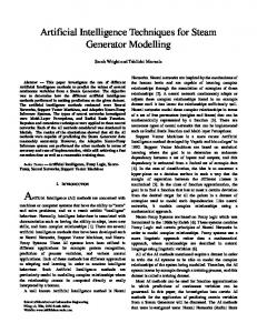
Figure 1 - DTI SAM toolset structure (Kellagher et al., 2009)

SAM Risk (see Figure 1) 1 and 2 are the user-interface and controller for the tool set, building the scenarios for SAM-UMC to process. SAM Risk 1 assumes full system functionality (no blocked or collapsed drains), whereas, SAM Risk 2 allows for the possibility of parts of the drainage system collapsing, or becoming blocked. The chance of a drain collapsing, or blocking, is calculated using an empirical equation (Long, 2008) for calculating pipe-failure probability. SAM-UMC then functions as an interface to the Infoworks CS COM object (Innovyze, 2007), which allows for the loading and running of simulations, from which the results can then be exported and collected. The rapid flood-spreading model distributes the excess water at each manhole (identified during the Infoworks CS run) over the terrain model. This project uses the SAM Risk 1 model, without taking into account the potential for drainage system collapse and blockage. SAM Risk 2 has a far larger demand on computational time, but produces very similar results to SAM Risk 1 on most networks (Kellagher, 2010). Further information on the function of the DTI-SAM tool set and calculation of risk can be found in chapter 3.

Page: 39

Chapter 2 – Literature Review

2.2.3 Flood Risk Management Summary In summary, risk-based methods of assessing flood risk are becoming more mainstream, and allow for a consequence-based evaluation of a flooding event, which gives a useful scale to measure how good a given drainage system is, compared to another. The DTI-SAM project previously completed at HR Wallingford has produced a useful tool set and methodology, which this project can build upon and incorporate in order to optimise flood-risk interventions.

2.3 Optimisation Algorithms 2.3.1 Introduction There are many kinds of optimisation algorithm, including: linear programming (Schrijver, 1998), integer programming (Schrijver, 1998), non-linear programming (Bertsekas, 1999), gradient descent algorithms (Baldi, 1995), evolutionary algorithms (Back, 1996) and swarm algorithms (Brownlee, 2012). In this chapter search algorithms are the main focus, which encompass some of the aforementioned types of algorithm. Search algorithms are designed to identify a desirable item, or items, amongst a superset of items. There are two main forms of search algorithm, deterministic algorithms, which are effective at solving simple problems and non-deterministic algorithms which are less efficient on simple problems. Non-deterministic algorithms can, however, solve considerably more complex problems that deterministic algorithms would either not converge on, or would not converge within a reasonable time. Deterministic algorithms encompass hill climbing or gradient descent algorithms Page: 40

Chapter 2 – Literature Review (Burges et al., 2005), the A* search algorithm (Liu and Gong, 2011) and TABU search (de Werra and Hertz, 1989; Gendreau and Potvin, 2005; Glover et al., 1993; Glover and Laguna, 1997; Hertz and de Werra, 1991; Soriano and Gendreau, 1996) amongst others. Non-deterministic algorithms encompass genetic algorithms (De Jong, 1975; Holland, 1975, 1962; Schaffer, 1985), simulated annealing (Kirkpatrick et al., 1983), and ant-colony optimisation (Dorigo et al., 1997; Dorigo and Blum, 2005; Dorigo and Stutzle, 2004; Gutjahr, 2000) amongst, again, a multitude of others. The problem this project is attempting to solve is highly complex and based on literature consulted, it is likely that deterministic algorithms would fail to converge to a good answer on the problem which this thesis solves in a reasonable time. This is because that problem is a non-linear, combinatorial, NP-hard problem, which are all characteristics of problems which deterministic algorithms do not solve well (Garey and Johnson, 1979). Therefore, deterministic algorithms will be ignored entirely, and only a brief overview of single-objective non-deterministic algorithms follows to set the scene, followed by an examination of the development and application of the powerful multi-objective techniques that would have a chance of obtaining a reasonably good answer to this project's problem within a sensible time frame.

2.3.2 Genetic Algorithms Genetic algorithms are based loosely upon Darwin’s theory of natural selection (Darwin, 1859), which suggests (to simplify greatly) that organisms evolve based on the more useful elements of an organism enabling that organism to breed Page: 41

Chapter 2 – Literature Review more, thus passing on those elements to some or all of its offspring, who will, again, breed more. Eventually the organisms with the useful traits will either supplant or exist alongside the original organisms. These useful elements would initially be produced by a mutation of existing elements, before being passed down parent to child in this manner. Genetic algorithms are immensely popular optimisation algorithms due to their suitability for non-linear, non-convex, multimodal and discrete problems with which traditional gradient descent derived algorithms may perform poorly in comparison (Nicklow et al., 2010). The process of a genetic algorithm can be separated into four distinct subprocesses: generation, selection, crossover and mutation. Generation involves building an initial population of potential solutions either by random creation or some other method. Selection is where the population is evaluated, and then a subset of that population is selected by one of many possible selection algorithms (e.g., fitness proportionate (Back, 1996), stochastic universal sampling (Ghimire et al., 2013), tournament selection (Miller and Shaw, 1996; Nicklow et al., 2010) etc.) for the generation of a child population via the next stages of crossover and mutation. Most modern implementations use either truncation or tournament selection (Nicklow et al., 2010) as these are scaling invariant and inherently elitist, which has been shown (Bayer and Finkel, 2004; Reed et al., 2000; Yoon and Shoemaker, 2001) to enhance the effectiveness of the genetic algorithm. Crossover is the process of generating new chromosomes by combining aspects from previous solutions chosen by the selection algorithm via one of several possible crossover algorithms (single-point, multi-point, uniform, partially mapped crossover, etc.) in the hope of producing a “child” chromosome more fit then Page: 42

Chapter 2 – Literature Review either of its “parent” chromosomes. Mutation involves introducing a chance of making random changes to the chromosomes, which helps to prevent premature convergence and allow a fuller exploration of the search space by including genes that were not present in the initial random population. A final process that is not essential to the function of the algorithm, but which vastly improves its efficiency and effectiveness, is called “elitism”. Elitism ensures that the best scoring chromosomes from each population make the transition from parent to child population intact. This ensures that promising search areas are not lost to the algorithm part way through iteration. Genetic algorithms have been around since the 1960’s (Holland, 1962). However, they only began to gain wider acceptance as an effective and efficient optimisation strategy in 1975. This was due to both the publication of “Adaptation in Natural and Artificial Systems” (Holland, 1975) and the thesis entitled “An analysis of the behaviour of a class of genetic adaptive systems” (De Jong, 1975). Holland (1975) presented the concept of adaptive algorithms utilising the concepts of mutation, selection and crossover, and De Jong (1975) showed that genetic algorithms could perform exceptionally well on discontinuous and noisy data that is challenging for many other optimisation techniques. Genetic algorithms have been utilised on many and varied problems since their development (Goldberg and Wang, 1997; Huang et al., 2009; Montana and Davis, 1989; Santarelli et al., 2006; Scully and Brown, 2009) with good success rates.

Page: 43

Chapter 2 – Literature Review

2.3.3 Simulated Annealing The annealing process in metalworking inspired the simulated annealing algorithm. Annealing is the process of heat-treating metal to achieve desired properties within the material by heating it up and then allowing it to cool very slowly. Annealing occurs because over time, the atoms within the metal align themselves towards the equilibrium state when the bonds between atoms have been broken (hence the heat). Simulated annealing (Kirkpatrick et al., 1983) is a computational emulation of this process, in order to apply it to optimisation problems. A temperature is tracked within the algorithm, beginning at a high level and gradually decreasing throughout the execution of the algorithm. The algorithm usually halts when the temperature reaches a pre-determined level. Initially, one solution to the problem in question is generated and the score obtained through the objective function represents the “energy” of that particular state. At each cycle of the algorithm, this state is altered to generate a new state. This new state is then evaluated and if its energy is lower, it replaces the current state. If the energy of the new state is higher, then it still may replace the current state, but that is based upon chance influenced by the current temperature and the difference in energy. As the temperature lowers, the chance of inferior solutions replacing the main solution drops swiftly (Smith and Savić, 2006). It has been proven (Geman and Geman, 1984) that with a sufficiently drawn out cooling schedule the simulated annealing algorithm will always converge to the best possible solution. Most implementations of simulated annealing are, Page: 44

Chapter 2 – Literature Review however, on far faster cooling schedules in order to be of use in providing an answer within a reasonable time frame. Simulated annealing does generally perform well over shorter intervals, however, and has proven to be an extremely effective solution for single objective optimisation problems.

2.3.4 Ant-Colony Optimisation Ant-colony optimisation is a relative newcomer to the field of optimisation algorithms, having been first introduced in the early 1990’s by M. Dorigo and his colleagues in Italy (Dorigo, 1992; Dorigo et al., 1997, 1991) as an algorithm for solving combinatorial optimisation problems. Like evolutionary algorithms, antcolony optimisation is a meta-heuristic algorithm inspired by nature. In this case, by the methods that ants in the natural world use to guide other members of their colony to discovered food sources, i.e., pheromone trails. When ants are exploring an area around their nest for food, they initially explore in a wholly random manner. When an individual ant discovers a food source, it evaluates the quantity and quality of this food source, and then carries a portion back to the colony’s nest leaving a pheromone trail behind it. The pheromone trail varies depending upon the quantity and quality of the food source. Other ants are attracted to follow this trail and will then discover the food and leave their own pheromone trail. The pheromones laid to mark these trails evaporate over time, so over time longer trails will become weaker than shorter ones and attract fewer ants in consequence. In this manner, although no direct communication has taken place, greater quantities of ants will be drawn towards the best food sources, the shortest distance from the nest (Dorigo and Blum, 2005). Page: 45

Chapter 2 – Literature Review Ant-colony optimisation has been applied to various problems successfully (Dorigo and Stutzle, 2004) since it was developed. A proof of convergence focusing on a particular implementation of ant-colony optimisation, called “Graph Based Ant System (GBAS)” to an optimum solution was published in 2000 (Gutjahr, 2000). This was followed by a more generalised proof of convergence to any optimal solution in 2002 (Gutjahr, 2002). Practical applications of GBAS have, however, been rare (Dorigo and Blum, 2005) and work continued on proving convergence of more commonly used ant-colony algorithms with an included positive lower bound. This has finally been completed with a proof for convergence in value and solution (Dorigo and Stutzle, 2004, 2002). Ant-colony optimisations main advantage over evolutionary algorithms, or other optimisation techniques, lies in its ability to be run on-line and swiftly compensate for live alterations to the problem being solved. It can be used with great effect for route planning, network planning, and similar problems, due to these capabilities. Evolutionary algorithms do, however, have a longer record of accomplishment and are considered a safer option, particularly where the problem has no element of volatility and does not have to be solved on-line.

2.3.5 Multi-Objective Optimisation The vast majority of optimisation algorithms are designed around the idea of a single objective; therefore, there is a proliferation of highly efficient, accurate algorithms to deal with single-objective problems that are highly documented (De Jong, 1975; Dorigo, 1992; Dorigo et al., 1997; Holland, 1975, 1962; Kirkpatrick et al., 1983). The field of multi-objective optimisation is more challenging and more Page: 46

Chapter 2 – Literature Review useful. Most real-world problems do not involve simply trying to find the most optimal approach to a problem to achieve one fixed solution. They are a matter of weighing different options against each other, based on several separate criteria, and attempting to select the approach with the most usable balance. Multi-objective optimisation algorithms are designed to work with more than one objective function. The algorithm works to minimise or maximise each of the objectives simultaneously. The objective functions are usually in conflict with each other, as if there was no conflict between the two objective functions it would be more efficient and possibly more accurate to develop a number of singleobjective optimisation algorithms and find the optimum value for each objective in this way (Coello, 1999). The issue of multi-objective optimisation is defined by (Coello, 1999) as finding the vector described in equation 1 where 2 and 3 are satisfied, the vector function in 4 is optimised, and the decision variable vector is as shown in 5.

∗ ∗ ∗ ! = # ,# ,…,# ) 1 2

*+ # ≥ 0 . = 1,2,3, … , 0

( 1 )

(

2

)

Page: 47

Chapter 2 – Literature Review

ℎ+ # ≥ 0 . = 1,2,3, … , 2

3 # = 34 # , 35 # , … , 36 #

# = #4 , #5 , … , #8

7

7

(

3

)

(

4

)

(

5

)

In words, multi-objective optimisation is the problem of finding from a given set, which satisfies the constraints listed in 2 and 3, the sub-set that is composed of the optimum values of all objective functions. This set is known as a “Pareto set” (Pareto, 1896), the non-inferior or non-dominated sets, which contain Pareto optimal solutions. A point is considered Pareto optimal if no vector exists which would improve the score of one criterion without causing a simultaneous deterioration in some other criterion.

2.3.6 Multi-Objective Evolutionary Algorithms The first mention of the concept of a truly functional multi-objective genetic algorithm (i.e., a genetic algorithm that could handle multiple objectives without resorting to objective function aggregation) dates back to the 1960’s (Rosenberg,

Page: 48

Chapter 2 – Literature Review 1967). However, no multi-objective genetic algorithm was developed at that time. An attempt was made in 1983 (Ito et al., 1983) to develop a multi-objective genetic algorithm, but usually credit is given to Schaffer with his Vector Evaluated Genetic Algorithm (VEGA) for developing the first fully functioning multi-objective genetic algorithm (Schaffer, 1985, 1984). VEGA offered a credible multi-objective genetic algorithm, but it failed to include a mechanism for multi-objective elitism. This dramatically affects the speed at which an algorithm converges to good solutions, as promising solutions may be lost throughout the process. After the development of VEGA, the most popular approaches for multi-objective genetic algorithms were aggregating functions. The most commonly used versions of these were the weighted-sum approach (Coello, 1999; Jones et al., 1993; Liu et al., 1998; Syswerda and Palmucci, 1991; Wilson and Macleod, 1993; Yang and Gen, 1994), goal programming (Charnes and Cooper, 1961; Coello, 1999; Ijirii, 1965; Sandgren, 1994; Wienke et al., 1992), goal attainment (Coello, 1999; Wilson and Macleod, 1993), s-constraint (Coello, 1999; Quagliarella and Vicini, 1997; Ranjithan et al., 1992; Ritzel et al., 1994). These aggregating functions had several common problems, including a difficulty in working well on non-convex search spaces. Furthermore, where weights were used within the algorithm a very good knowledge of the objective functions in question was required for the values of those weights to be decided. So the need for improvement in the field was still very obvious. The initial ideas of including the concept of pareto-optimality in multi-objective algorithms arose in Goldberg’s book in 1989 (Goldberg, 1989). Whilst criticising Page: 49

Chapter 2 – Literature Review VEGA, he suggested that the use of non-dominated ranking of solutions with selection could move a population towards the Pareto front. There was no implementation of this idea for an algorithm supplied, but the majority of multiobjective algorithms developed after the publication of this book drew in a large part upon his ideas and suggestions (Coello, 2005), most notable the nondominated sorting genetic algorithm (NSGA) (Srinivas and Deb, 1994), the niched Pareto genetic algorithm (Horn et al., 1994), and the multi-objective genetic algorithm (MOGA) (Fonseca and Fleming, 1993). Additionally, in 1992 a method was developed (Tanaka and Tanino, 1992) to incorporate user preferences into a multi-objective evolutionary algorithm. From this point onwards, a focus shift occurred. The problem of building effective algorithms had been solved, and the goal was now to produce ever more effective and efficient algorithms (Coello, 2005). One of the main initial steps moving towards efficiency and effectiveness was the introduction of elitism to the multiobjective evolutionary algorithm playing field. Elitism involves artificially preserving the most optimal chromosomes produced at each point where chromosomes may be lost from the algorithm process, to ensure that promising solutions are not lost. Although early studies hinted at the possibility of application of elitism to multi-objective evolutionary algorithms, the formal introduction of this concept to the subject is usually credited to Echart Zitzler (Zitzler and Thiele, 1999) and his strength Pareto evolutionary algorithm (SPEA). After the publication of Zitzler’s paper the majority of multi-objective evolutionary algorithms implemented some form of elitism (Coello, 2005). The most common form of elitism within a multi-objective evolutionary algorithm involves an external Page: 50

Chapter 2 – Literature Review population comprised of all generated non-dominated solutions. Every solution entered into the external population must be non-dominated with regard to that population, and replaces any solution that it dominates within it. The most popular current multi-objective evolutionary algorithms are SPEA (Zitzler and Thiele, 1999, 1998), SPEA2 (the second iteration of SPEA) (Zitzler et al., 2002), the pareto-archived evolution strategy (PAES) (Knowles and Corne, 2000), and NSGA II (the second iteration of NSGA) (Deb et al., 2002, 2000).

2.3.7 Multi-Objective Simulated Annealing Although attempts have been made to convert simulated annealing to multiple objective optimisation due to its effectiveness as a single objective algorithm (Bandyopadhyay et al., 2008; Smith and Savić, 2006), it does not lend itself to the concept in the same way as evolutionary algorithms do, with their large population based approach. Attempts have generally revolved around objective function aggregation, similar to earlier multiple-objective evolutionary algorithm attempts (Smith and Savić, 2006).

2.3.8 Multi-Objective Ant-Colony Optimisation Similarly, to multi-objective simulated annealing, attempts have been made to develop multi-objective ant-colony optimisation algorithms (López-Ibáñez et al., 2004; López-Ibáñez and Stützle, 2012; López-Ibáñez and Stutzle, 2010). Antcolony optimisation does not, however, lend itself so conveniently to multiobjective optimisation and finding Pareto sets as evolutionary algorithms do. Additionally, ant-colony optimisation is a fairly recent algorithm and does not have Page: 51

Chapter 2 – Literature Review a comparable body of published applications to some other algorithms to back up its effectiveness.

2.3.9 Optimisation Algorithms Summary In summary, there are an extremely large amount of optimisation algorithms available, even when discussing multi-objective optimisation. Genetic algorithms in general have been used for many applications, and are particularly suited for adaptation to multi-objective optimisation, due to population-based manner in which they operate. Ant-colony optimisation methods have the same benefit but have fewer real-world successful applications to date. NSGA-II has a proven track-record of published applications to various problems (Behzadian et al., 2009; Bekele and Nicklow, 2007; Kannan et al., 2009). It has also been applied successfully to water-distribution problems (which have some similarities to drainage problems) as the base of promising heuristic optimisation algorithms (Behzadian et al., 2009; di Pierro et al., 2009; Fu and Kapelan, 2010; Jourdan et al., 2005, 2004).

2.4 Machine Learning 2.4.1 Introduction Machine learning is a branch of artificial intelligence techniques dealing with algorithms that can learn from data. The most common usage is for data mining, and they can be used to great effect for classification of data (Kotsiantis, 2007). There are two main types of learning undertaken by machine learning algorithms,

Page: 52

Chapter 2 – Literature Review commonly referred to as “supervised” and “unsupervised” learning (Kotsiantis, 2007). Data sets for training machine learning algorithms may be continuous, categorical, or binary. Where instances within the data set are provided with known labels (i.e. the correct outputs) the training process is known as a “supervised” process (Kotsiantis, 2007). Where there are no known labels, the process is known as “unsupervised” (Kotsiantis, 2007). Algorithms designed to undertake unsupervised learning generally work with clustering techniques such as Bayesian techniques (Neal, 1995). Clustering techniques are methods of identifying similarities between data instances. Those instances are then given (often varying degrees of) membership of “clusters” in an attempt to identify unknown but potentially useful classifications of data. These have been used on such diverse problems as road sign recognition (Prieto and Allen, 2009), water resources (Kalteh et al., 2008) and text detection with character recognition (Coates et al., 2011). In this thesis the concentration is on classification algorithms, specifically artificial neural networks, and supervised training. This is because part of the work performed will be following on from previous work on developing neural network meta-models for multi-objective optimisation (Behzadian et al., 2009). Additionally, the second area where machine-learning techniques are utilised is within the LEMMO (Learning Evolution Model for Multiple-objective Optimisation) algorithm (Jourdan et al., 2005). The LEMMO algorithm is designed in the same way as the LEM algorithm that it was built upon (Michalski et al., 2000) to utilise

Page: 53

Chapter 2 – Literature Review any machine-learning algorithm. Artificial neural network (ANN) code was already implemented, so ANNs will be utilised for the machine learning part of this algorithm to minimise development time.

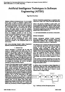
2.4.2 Artificial Neural Networks The first neural network model which featured digital neurons was developed as early as 1943, although in this model no capability for learning was initially included (McCulloch and Pitts, 1943), limiting the usefulness of the model. In 1958 Frank Rosenblatt developed the “Perceptron” model (Rosenblatt, 1958), however Rosenblatt was unable to identify a reliable mathematically accurate mechanism for allowing multi-layer perceptrons to learn. The next major advance in artificial neural networks occurred in 1974, when Werbos (1974) succeeded in discovering the back-propagation algorithm, which was also independently rediscovered in 1982 (Parker, 1982). The application of neural networks to varied and complex problems is, today, a common occurrence (Behzadian et al., 2009; Biswajeet et al., 2010; Rowley et al., 1998). There are two methods of training an artificial neural network – supervised and unsupervised (Kotsiantis, 2007). Supervised learning requires a set of training data that is pre-processed such that, along with each instance of data, there is an included expected output for the artificial neural network. The most common model for supervised-learning neural networks architecture is a feed forward network (see Figure 2). This is an arrangement of different layers of “nodes”, most commonly an input layer, a “hidden” layer, and an output layer. Each layer within

Page: 54

Chapter 2 – Literature Review this arrangement has connections to the outputs of nodes of the previous layer, and each of these connections has an associated weight (Lippman, 1987).

Figure 2 - Feed forward artificial neural network structure using a sigmoid activation function

Data then enters into the network at the “input” points (see Figure 2) and proceeds through the network node by node. At each connection it is multiplied by the value of the weight attached to that connection. At each node it is processed by a function – usually a differentiable function to facilitate training, of which the most popular are the logistic function (sigmoid function, see equation 6), and the Gaussian function (see equation 7). Artificial neural networks using Page: 55

Chapter 2 – Literature Review sigmoid or Gaussian functions have been shown to be capable of approximating any arbitrary continuous function on a limited size domain, with varying accuracy depending on the number of neurons in the network (Cybenko, 1989; Hartman et al., 1990; Hornik et al., 1989; Park and Sandberg, 1991). Indeed, it has been shown (Hornik, 1991) that the choice of activation function is not as critical in allowing for the potential of universal approximation as the feed-forward architecture.

9 : =

1 1 + < =>

3 # = ?< −

#−A 2B 5

5

+C

(

6

)

(

7

)

Training of feed forward artificial neural networks is accomplished by modifying the weights within the network to move them closer to achieving a desired output. The most commonly used algorithm to achieve this is the back-propagation algorithm (Parker, 1982; Rumelhart et al., 1986; Werbos, 1974). Backpropagation is a supervised learning technique that involves propagating error backwards through the network. It is a gradient descent method and because of this in its pure form it will be trapped at any localised optima that occur in the search space. A nearly ubiquitous addition to back-propagation in order to avoid this effect is “momentum” (Rumelhart et al., 1986). Momentum allows the backpropagation algorithm to be influenced by recent trends in the error surface, Page: 56

Chapter 2 – Literature Review reducing the likelihood of, but not eliminating, the possibility of being stuck in local optima. Back-propagation can be viewed as a simple gradient descent algorithm optimising the weights with the error from the artificial neural network performing the role of an objective function to be minimised. Taking this viewpoint makes it clear that any optimisation algorithm could be utilised to the same purpose. Genetic algorithms (see 2.3.2), simulated annealing (see 2.3.3), ant-colony optimisation (see 2.3.4) or any other optimisation algorithm can also be utilised, therefore, as part of the training process of an artificial neural network (Montana and Davis, 1989). This is also true for other versions of error propagation algorithms (Heaton, 2014; Igel and Hüsken, 2000).

2.4.3 Bayesian Belief Networks Bayes’ rule is a mathematical rule, which identifies the way in which existing beliefs should be altered, given a set of evidence previously unavailable. This can be simply illustrated with an example utilising white/black marbles as measures of belief. If it is imagined that a new-born baby sees the sun set, and wonders whether it will rise again. As the child has no prior knowledge, it assigns a fiftyfifty chance that the sun will rise again the next morning, and represents this by placing a white marble and a black marble into a bag. The following day, the sun does rise. The child, therefore, places another white marble into the bag to represent his increase in belief that the sun will rise. The probability that a random marble selected from the bag will be white (i.e. the child’s belief that the sun will rise), has gone from 50% to 66.67%. As time passes and the bag becomes nearly Page: 57

Chapter 2 – Literature Review entirely full of white marbles, the child becomes increasingly convinced that sunrise will come each day (Anonymous, 2000). Mathematically, this can be represented as in equation 9 (Bayes and Price, 1763; Laplace, 1986) where equation 8 denotes the probability that a random variable ‘R’ has the value ‘r’ given that the evidence is equal to ‘e’.

D E = F|