ARTIFICIAL NEURAL NETWORK ALGORITHMS FOR ACTIVE NOISE CONTROL APPLICATIONS PACS: 43.50 Ki
FERNÁNDEZ FERNÁNDEZ, ALEJANDRO; COBO PARRA, PEDRO Instituto de Acústica. CSIC. C/ Serrano 144 28006. MADRID SPAIN Tfn: 34-91-561 88 06 Fax: 34-91-411 76 51. E-Mail:
[email protected]
ABSTRACT This paper shows the use of several methods commonly applied to training Artificial Neural Networks (ANN) in Active Noise Control (ANC) systems. Although ANN are usually focused on off-line training, real-time systems can take advantage of modern microprocessors in order to use these techniques. A theoretical study of which of these methods suit best in CAR systems is presented. The results of several simulations will show their effectiveness.
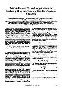
INTRODUCTION The objective of Active Noise Control or ANC systems is to generate an acoustical signal or “anti-noise” that is capable of cancelling the primary noise when both signals interfere. This task is accomplished by the use of electronic controllers which are able of filtering a reference signal (feedforward ANC) or the error signal (feedback ANC) so that their output (secondary signal) cancels the primary noise. This type of controllers usually needs to estimate transfer functions between the different outputs and inputs of the system (figure 1). This estimation is commonly done by the use of a FIR or IIR filter whose weights are adapted in order to minimize an error signal; a noise signal is emitted through the secondary source and measured by the error
microphone. It also e f eds the adaptative filter as reference signal. The controller then tries to minimize the sum of the error microphone signal and the output of the filter, normally using an LMS (Least Mean Square) steepest-descent algorithm applied to the instantaneous error.
Although simple and stable, the LMS algorithm and its variations (normalized LMS, leaky LMS, etc.) are slow. The speed of their convergence depends on the step size (µ), as can be seen in the weight actualization equation:
W ( k + 1) = W ( k ) + µ·e(k )·X ( k ) Error (e) Primary S.
P. Path
Reference (x)
+-
Secondary Source
W1
Estimate S.P. Weights W2
++
Measurement Noise
S. Path
W2
Figure 1: FXLMS controller scheme. This controller needs an estimation of the secondary path (transfer function between the secondary source and the error microphone).
The maximum value of the step size is a function of the power of the reference signal X and the number of weights (Widrow and Stearns, 1985):
0