Artificial Neural Network and Support Vector Machine ... - IEEE Xplore

710

IEEE TRANSACTIONS ON POWER DELIVERY, VOL. 20, NO. 2, APRIL 2005

Artificial Neural Network and Support Vector Machine Approach for Locating Faults in Radial Distribution Systems D. Thukaram, Senior Member, IEEE, H. P. Khincha, Senior Member, IEEE, and H. P. Vijaynarasimha, Student Member, IEEE

Abstract—This paper presents an artificial neural network (ANN) and support vector machine (SVM) approach for locating faults in radial distribution systems. Different from the traditional Fault Section Estimation methods, the proposed approach uses measurements available at the substation, circuit breaker and relay statuses. The data is analyzed using the principal component analysis (PCA) technique and the faults are classified according to the reactances of their path using a combination of support vector classifiers (SVCs) and feedforward neural networks (FFNNs). A practical 52 bus distribution system with loads is considered for studies, and the results presented show that the proposed approach of fault location gives accurate results in terms of the estimated fault location. Practical situations in distribution systems, such as protective devices placed only at the substation, all types of faults, and a wide range of varying short circuit levels, are considered for studies. The results demonstrate the feasibility of applying the proposed method in practical distribution system fault diagnosis. Index Terms—Artificial neural network, distribution systems, fault location, support vector machines.

I. INTRODUCTION

D

ISTRIBUTION SYSTEM (DS) consisting of a number of radial feeders, has to be highly reliable and efficient under normal and contingency conditions. In the event of fault there should be exact information about the type of fault and its location. This information is required to start the network reconfiguration, as soon as possible and restore normal energy supply. Hence, one of the crucial blocks in the operation of such a DS is that of fault detection and its location. This objective is achieved and depends on the success of the Distribution Automation (DA) System and in turn on the availability of reliable measurement database from SCADA systems. The DA system should be implemented quickly and accurately in order to isolate those affected branches from the healthy parts and to take countermeasures to recover normal power supply. DA analytical tools include various application functions [1], [2]. Faults are abnormal events that frequently occur in distribution feeders. Distribution feeder faults modulate primary current and generate noise through arcing phenomena. Owing to their nature (presence of low or no current), the conventional protection scheme is not capable of detecting them. Usually they are

Manuscript received March 31, 2004; revised June 24, 2004. Paper no. TPWRD-00151-2004. The authors are with the Department of Electrical Engineering, Indian Institute of Science, Bangalore 560 012, India (e-mail: [email protected]). Digital Object Identifier 10.1109/TPWRD.2005.844307

identified only when the consumers inform the utility about a broken cable or complain about the cut in power supply. Traditional outage handling methods were based on the customer trouble calls [3]. The geographic location of the caller and the connectivity of the distribution network have to be overlapped exactly for the exact location of fault. Also, there might not be any calls during night-time, which poses a problem for the operator in locating the fault. Also, the available measurements of currents in the lines and voltages at the distribution transformers may be limited, e.g., situations such as communication failures or due to other practical difficulties of installing measuring devices at each DS bus. Hence, it is of practical importance that the exact location of fault is estimated only with limited measurements available around the substation. In recent years, some important techniques have been discussed for the location of faults particularly in Radial Distribution systems [4], [5]. These methods use various algorithmic approaches, where the fault distance is iteratively calculated by updating the fault current. Measurements are assumed to be available at the sending end of the faulty line segment. The emerging techniques of Artificial Intelligence (AI) can be a solution to this problem, wherein all the short circuit analysis are carried out offline, and the fault is located online within short time. A brief comparison of various analytical techniques with the ANN method for fault location in Transmission System is provided in [6]. Among the various AI based techniques like Expert systems, Fuzzy Set and ANN systems, the ANN approach for fault location in transmission lines is found to be encouraging [7]–[9]. The major bottlenecks in Fault Location, particular to Distribution System are: • Very limited measurements along the path of the feeder. The limiting case being of measurements only at the substation. • No Circuit Breaker (CB) and relay statuses, and measurements of each line segment, unlike the Transmission System. • The number of generators in operation changes throughout the day and so, the measurements obtained during fault at a specific location, but at different times of a day, are different. The Function Approximation procedure must overcome these difficulties for the success of the DA. Artificial Neural Networks (ANNs) have been successfully applied for Fault Section Estimation (FSE) [10], [11], where the information of the current

0885-8977/$20.00 © 2005 IEEE

THUKARAM et al.: ARTIFICIAL NEURAL NETWORK AND SUPPORT VECTOR MACHINE APPROACH

status of protective relays and CBs are available. These techniques have been more popular in the Transmission Systems. Section II describes the Short Circuit analysis of the Distribution System with loads. A functional relation between the driving point impedances of buses and the substation measurements is developed in this section. Section III gives brief description of the proposed methodology, some schemes relevant to the problem, and describes the ANN and SVM approach used for the present problem. PCA based data preprocessing, particular to this problem, is outlined in Section IV. The test system and the results of the proposed approach are presented in Section V. II. FAULT LOCATION ALGORITHM There is a definite relation between the measurements at the sending end, and the distance of fault from this end, for the faulted phase. On the source side, in the case of a distribution system, an equivalent generator is modeled with an equivalent reactance, at the sending end of the radial feeders. The varying number of generators in operation is modeled by an equivalent reactance at this bus. Varying this equivalent reactance in a specified range varies the contribution of short circuit MVA from the source side. Consider a fault of a general type occurring on a bus (or on a line section) at a distance of p from the Source side, as shown in are voltages at bus i, initially and during fault Fig. 1. conditions. is Driving Point Impedance of bus i. are fault current, fault impedance. during fault voltage at fault point p. (1)

711

from the sending end. (The distance is implicit of the terms and ). In simple analogy, (6) is (7) where

is a function relating the distance of fault node from the source, and the corresponding terms of the Z-bus matrix. The relation in (7) will become complex, once varying load conditions, fault resistance, and different types of faults on a feeder, are incorporated. This function would then correspond to numerous inputs mapping onto a single target, e.g., a single line to ground fault occurring at the same location on a feeder, but at different load levels. Such type of mapping is difficult to model using an algorithmic approach. Hence, this paper proposes a new, combined approach, wherein the Support Vector Machine (SVM) breaks the complexity of (7), and the ANN (in this case, Feedforward neural network) estimates the unknown parameters in (7) based on supervised learning. Also the purpose of this paper is to show that a very limited and reliable set of measurements can lead to a very accurate estimation of the fault location, considering the various practical aspects of the DS. Any further information regarding the fault, i.e., statuses of various switches and CBs in the path of the feeder can be effectively added to the input space, so that the actual fault location can be determined among multiple fault locations. The high impedance faults can be simulated over a range of impedance values. This becomes a further more complex functional relation.

Voltage of bus i during fault is (2)

A. Proposed Approach

Similarly voltage at fault point p during fault is (3) Substituting (1) in (3), (4) The fault current is obtained as (5) Substituting the value of

III. ARTIFICIAL NEURAL NETWORK AND SUPPORT VECTOR MACHINES BASED FAULT LOCATION

from (5) in (2) (6)

This is the value of voltage at bus i, during steady state fault conditions. From (6), it is seen that, the voltage at bus i during fault is a function of initial voltage at buses i and p, driving point impedance of bus p, transfer impedance between buses i and p, as a measurement and the fault impedance. By considering at the sending end, we obtain the distance of the faulty bus p

The relationship between the measurements and the fault distance is highly complex if all types of faults at all loading levels and, along all the radial feeders, are considered simultaneously. The faulty feeder can of course be identified by the status of the protective device at the substation. Now, consider a system as shown in Fig. 11. There are 3 radial feeders, with 52 nodes, where each node is a distribution transformer with a specified load. Consider a single line to ground fault on a node (say node 8) of feeder 1. During fault, the 3 phase voltage and current measurements at the substation are considered as the input vector and, the line reactance of the feeder up to the node 8, is considered as the target. This is repeated for other nodes of the feeder 1. The relation between these measurements and the targets are built up by the ANN, which relates them only in a condition of one fault type and at one Source Short Circuit (SSC) level. To consider different types of fault and a range of SSC levels, we need to map multiple inputs to a single output. This becomes difficult to model using a single ANN. This can be seen from Fig. 10, i.e., variation of data points in the input space and the difficulty involved in mapping such a space. Hence we model the single input, single output type of mapping, e.g., single line

712


Fig. 1. Three-phase Radial network with general fault at distance p from the source side.

to ground fault at a known SSC level occurring on a node. For this, we need to know the type of fault and the SSC level prior to the estimation of the fault distance by the ANN. This is solved as a classification problem using techniques such as Support Vector Machines, which have well-established advantages over other classification methods. Multiclass classification [12]–[14] is adopted for both fault type (4 types of faults) and SSC level (7 classes of SSC levels) classification. Here, two schemes are proposed for locating the fault. In scheme I only fault type classification is done, and all SSC levels are considered with in one ANN. In scheme II, the fault type and SSC level are determined by the classification procedures and there is a one-to-one mapping, which is then modeled by the FeedForward Neural Network.

Fig. 2.

Block description of Scheme I.

Fig. 3.

Block description of Scheme II.

B. Training Patterns The data used in the supervised learning are obtained at the substation. We have considered the three-phase steady-state voltage and current signals as measurements. The SSC level at the source bus (substation) is varied in specific steps to simulate the DS under light load conditions up to peak load conditions. The range of SSC level used for simulation is from 20 MVA to 50 MVA, in steps of 5 MVA. Hence we get 7 SSC levels: 20, 25, 30, 35, 40, 45, and 50 MVA. Similarly, 4 types of faults, Line to Ground (LG), Double Line to Ground (LLG), Line to Line (LL) and 3-phase Symmetrical faults are simulated at each load point (bus) on the Distribution Network. Measurements are taken at each of the above DS conditions. Scheme I: In this scheme, multiclass classification is done based on the fault type. A Support Vector Classifier is trained for this purpose, with input patterns obtained by simulating all types of faults at the nodes of a feeder. The block diagram of scheme I is shown in Fig. 2. In this figure the 4 blocks “ANN a” to “ANN d” correspond to ANNs trained with patterns obtained corresponding to the 4 types of faults. Each ANN block approximates the function relating the input vectors and the targets, for all SSC levels that are considered during short circuit analysis. Hence, without explicitly knowing the SSC level at the time of fault, the fault location is estimated in this scheme. Scheme II: In this scheme, Support Vector Classifiers are trained with the patterns obtained during fault simulation with all types of faults and the entire range of SSC level. After training, these classifiers determine the fault and SSC level of a fault online. Hence, the work of the FFNN is reduced

to modeling of a simple one-to-one mapping. The block diagram of scheme II is shown in Fig. 3. In this figure the block ‘ANN 1a’ represents an ANN trained with patterns obtained at 20 MVA SSC level and fault of type Line to Ground. Hence there are 7 4 (7 SSC levels, 4 types of faults) ANN blocks. The fault type classifier SVM is trained to classify the type of fault. Also, there are 4 SVM blocks trained to classify the SSC level of the input, where each block corresponds to a particular type of fault. Though the ANN and SVM blocks are more in number, in this scheme compared to scheme I, training is faster due to the lesser number of training patterns for each ANN and SVM block. As training of all the blocks runs in parallel, with reduced number of training patterns, offline training of scheme II is faster. Detailed steps followed in scheme II are described as follows: Step 1: Fault of a type is simulated at each node on a feeder with a particular SSC level, say 20 MVA at the source, and measurements are collected at the substation. Step 1 is repeated for each node, for all types of faults and the complete range of SSC level from 20 MVA to 50 MVA.


713

Step 2: The input vectors and the targets corresponding to a feeder are normalized as outlined in Section IV. Steps 1 and 2 are repeated for other feeders. Step 3: There is some amount of redundant information in the input set. The redundancy exploring proves useful in case the dimension of the input vector is high, e.g., in the case of more measurements available along the path of the faulty feeder. The architecture of the ANN for such data of reduced dimension is simple and its training is faster, without much compromise on the accuracy of the results. For dimensionality reduction, consider a feature matrix, with training patterns as its columns. A covariance matrix of the input dataset is obtained. The reduced input dataset is obtained by multiplying the original feature matrix, with the eigenvectors of the covariance matrix that correspond to significant eigenvalues. This means that we consider only those dimensions of the input space that contribute maximum to the information contained in the dataset. Step 4: Support Vector Classifiers are trained to classify the fault type and the SSC levels. Step 5: The input vector corresponding to a fault type, a SSC level, and a feeder is passed on to an ANN block for training. The target for each node is provided. The Procedure for online Fault Location is outlined in the form of a flow chart shown in Fig. 4.

C. ANN Methodology

Fig. 4.

Flowchart representation of the online fault location process.

Fig. 5.

Typical Feedforward Neural Net used in the proposed approach.

The ANNs have emerged as powerful tools for function approximation [15], and control of dynamical systems [16]. This is because of the advantage of high computation rate provided by their massive parallelism and, versatility of the three-layered FeedForward Neural Networks (FFNN) in approximating a complex nonlinear mapping. The fault location problem of radial distribution systems has two distinct features, which qualify the ANN approach as the preferred one, among other AI techniques. •

Huge dataset corresponding to a vast Distribution Network. • The complex relation between the input dataset and the target set. The ANN used is the 3-layered FFNN whose architecture is shown in Fig. 5, with activation functions for the hidden and output layer neurons as the nonlinear e.g., tangent hyperbolic and the linear transfer functions retransfer function spectively. Number of hidden neurons is chosen to match the complexity of the function, which it emulates. The Training algorithm used is the well-known Levenberg Marquardt (LM) algorithm [17], due to its proven advantages over other conventional methods, like faster learning, reliable convergence. The LM algorithm is basically a Hessian-based algorithm that allows the network to learn more subtle features of a complicated mapping. The training process converges quickly as the solution is approached, because the Hessian does not vanish at the solution.

The Error function or Cost function chosen for the learning process is the mean squares of the error of the outputs, along with a regularization term, which increases the generalization ability of the neural net. This is of more relevance in this context as faults can occur at any point between two buses that are chosen for learning the function. The regularization term used is the mean of the sum of squares of the network weights.

714


TABLE I SAMPLE TWO-CLASS CLASSIFICATION OF 3-PHASE SYMMETRICAL FAULTS ON FEEDER 2

Fig. 6.

SSC level classification of Feeder 2.

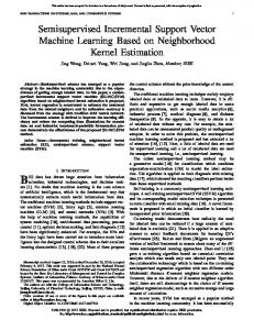
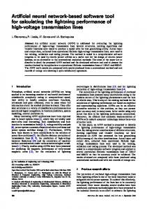
However, the advantages of ANN in the Fault Location process suffer a major setback when encountered with the situation of varying SSC levels in a Practical Distribution System. Due to this condition of the DS, a fault occurring at a specific location, though representing the same location, does not have the same target to map to. The target, if drawn from the Z-BUS impedance matrix, leads to this situation. Therefore the line reactances are chosen as targets to the fault locations. Further, there is the difficulty that the SSC levels are unknown, unless of course the utility gets this information from the control center each time the fault occurs. This disadvantage can be eliminated by the prior classification of patterns on the basis of a complete range of SSC levels. This leads to the information about the level at which the fault occurs, knowing which, the output of the ANN can be recognized as the true one. D. Support Vector Machines Methodology In recent years, Support Vector Machines (SVMs) [18] have risen as powerful tools for solving classification and, regression problems [19], [20]. SVMs try to find the hyperplane, which separates optimally, the training patterns according to their classes, which have been previously mapped to a high dimensional space, such that structural risk is minimized. Traditional quadratic programming algorithms [20] have been proposed, but these algorithms require enormous matrix storage and do expensive matrix operations. To avoid these problems, fast iterative algorithm like the Sequential Minimal Optimization (SMO) [21], which is easy to implement is chosen for training the SVMs. A sample Support Vector Classifier (SVC) is described in 2D space by simulating 3 phase symmetrical faults at the 12 nodes of feeder 2 of the test system described in Section V. The output of the SVC, classifying the patterns based on their SSC levels is shown in Fig. 6. If n is the number of SSC levels that are simulated, then the number of classifiers chosen is . Thus, there are 6 binary classification problems for each of the SSC level classifiers ‘SVM a’ to ‘SVM d’ to solve during training process, e.g., Classifier 1 classifies faults of 20 MVA and 25 MVA. ‘SVM a’ in Fig. 3 refers to SSC level classifier that is trained with Line to Ground faults. The function value in (A6) points to the class the pattern belongs to i.e., each SVC outputs the pattern as a positive or negative function value, which

TABLE II CLASSIFYING 3-PHASE SYMMETRICAL FAULTS OF TWO LEVELS ON FEEDER 2

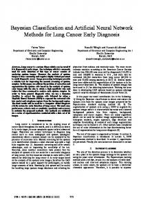
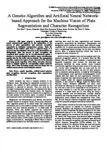
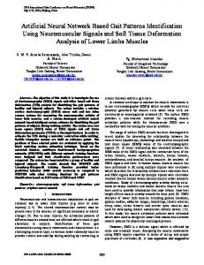
is indicative of it belonging to either class. Output of Classifier No 3 i.e., SVC classifying faults at 30 MVA and 35 MVA levels is given in Table I. The patterns corresponding to nonzero Lagrange multipliers are the support vectors, which define the separating hyperplane. Table II, describes the classification of 32 MVA and 33 MVA source level faults as that of 30 MVA and 35 MVA source levels respectively. The results correspond to 3 phase symmetrical faults of levels 32 MVA and 33 MVA, simulated on the midpoint of line connected between nodes 30 and 31. The value of the 32 MVA fault changes sign at classifier nos. 2, 3 (in third column of Table II—the value of changes from—2.4922 to ) and the common class between these two classifiers being 30 MVA, we classify this fault as one that occurred in the group of 30 MVA. Similarly for the 33 MVA fault, which is categorized as belonging to 35 MVA class. Similarly, in the fault type classifier, the patterns are classified into 4 classes as shown in Fig. 7. Now the fault is completely specified, in the sense that, its type and SSC level being known, the trained Feedforward Neural Network can estimate its location accurately. Another SVC is trained to classify the input pattern as belonging to a nearby node, i.e., fault occurring in the vicinity of the node and output of the trained SVC is shown in Fig. 8. Combining the three SVCs: Fault type classifier, SSC level classifier, Fault bus classifier described above, we get a stand alone SVM Fault Locator System. However, we describe here a scheme to show how the exact location of fault is determined using a combined approach.


Fig. 7.

Fault-type classification by an SVC.

715

However the current measurements of the three phases are normalized, to bring them within the range of 0.0 to 1.0. To get a feel of the pattern of scattering of data points in the input space, we shall show the input space in 3D. When more measurements are available to the Distribution System, the input dimension can increase, sometimes resulting in high redundancy, and more training times of the ANN and SVM. The variable reduction or dimensionality reduction comes to help under such conditions. The dimensionality reduction is carried out using the Principal Component Analysis (PCA) technique. A low-dimensional feature vector is a critical element in any pattern recognition problem as the number of data examples needed for training grows explosively with the dimension of the problem. Care must be taken at this stage that the information discarded in the dimension reduction is not relevant for diagnosing the fault. The PCA, which is a feature reduction technique is fast, simple and is characterized by minimal loss of information. : size of the input vector : dimension of the input vector : th element of input vector corresponding to th dimension. The initial feature matrix

with column vector Fig. 8.

Fault bus classification of Feeder 2.

The circled points in the Figs. 6, 7, and 8 are the support vectors that define the separating hyperplanes, lines or curves in the case of 2 dimensional space. The classification problem is: learning these separating hyperplanes. A brief mathematical derivation of the binary classification problem is outlined in the Appendix A. IV. DATA PREPROCESSING

of dimension d is adjusted to have zero mean, and unit variance by subtraction from each dimension (row), the mean of that dimension. Thus,

where, Mean Standard Deviation (SD) of

, is

The data and targets are normalized by dividing the current values by a suitable constant or can be done as follows: The covariance matrix of the feature matrix is calculated as where normalized input; raw input;

(say). Here, represents each element of the input vector and also that of target vector. The targets in this case are scalar. The elements of the input vector that are well within the range of 0.0 to 1.0 are not normalized, e.g., per unit voltage measurements.

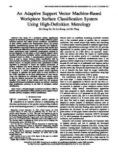
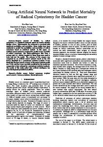
In general, the dimensionality of the dataset is reduced to the number of significant eigenvalues of the covariance matrix. Though these dimensions do not have any physical meaning in the fault location problem, they depict the most important aspect of the function approximation problem, i.e., the way in which the data are scattered in the reduced dimensional space. In Fig. 9 the data points of LG fault are shown in 3D space along the 3 major eigenvectors. The solid line connecting the points depicts the variation of the fault distance along the path

716


Fig. 9. Dataset of LG faults on Feeder 1.

Fig. 10. Dataset of Feeder 1, corresponding to the overall fault location problem.

of the feeder, whereas the dotted line depicts the variation of data points over the range of SSC levels. The points are arranged in the order of the targets, which they represent. We note that the surface has a well-defined shape, which can be modeled by the neural net. Scheme I models the whole surface, whereas Scheme II models each solid line independently. In Fig. 10, each point represents a fault of a particular type and at a particular SSC level, on a node of Feeder 1. From this figure we can conclude that a single ANN, that is required to map each of these points to the respective targets, cannot handle the Fault Locating Scheme efficiently. So, as a first step in the Fault Location process, the faults are classified by their type. A fuzzy type of logic can do this classification, but in this paper the Support Vector Machines (SVM) approach is used. As the size of the Distribution Network grows, the Fault Location system deals with huge datasets, which have to be classified into various classes and subclasses. The SVM shows its strength as a pattern classifier under these demanding situations. V. TEST SYSTEM AND RESULTS The developed algorithms are tested on a few Distribution Systems. Results obtained on a sample 11 KV Practical Distribution Network of 52 buses with 3 main feeders shown in Fig. 11 are presented. Each feeder of the system consists of more than one main branch. The Loads in kVA are represented by the distribution transformers at various nodes.

The simulated short circuit levels are 20 000 kVA (light load conditions) through 50 000 kVA (peak load conditions), in steps of 5 000 kVA. The value of this step change in SSC level can be chosen in accordance with the required accuracy of the function approximation. Each feeder is analyzed individually. Measurements are collected at the substation (Bus 1) for simulated faults on each node of a feeder. In the case of multiple branches e.g., 4 branches of feeder 2, the fault location is estimated to be on more than one branch of the feeder. To know the true fault location we need to know the statuses of the switches and fuses that are encountered along the path of the feeder. A sample problem of the above type is shown in Fig. 12 with results in Table III. The input vectors, targets and the corresponding outputs (in reactance), for faults of type single line to ground at two SSC levels, and at all the nodes of feeder 1, are shown in Table IV. In Fig. 13 the absolute error distances i.e., deviations of the estimated location of fault from actual Fault Location in meters, of Scheme I are shown. The errors correspond to the simulated fault locations at the nodes on feeder 1. The errors in case of Scheme I are in the range of 100 to 300 meters. But when each ANN encounters an SVM-classified fault described in Scheme II, we see from Fig. 14 that the error distances are reduced to a negligent value of about 10 meters. The simulated fault locations in Scheme II are: 20%, 50% and, 80% of distance on each line segment of a feeder. Results for the Peak load and Light load conditions are included. Also, this shows that the proposed scheme II is better than scheme I for the present problem. The performance errors (with regularization included), number of training epochs of the Feedforward Neural Network and, the architecture of the Feedforward Neural Network (FFNN), for schemes I and II are shown in Table V. It is seen that the 3-layered FeedForward Neural Network and the SVM network perform exceedingly well under various practical conditions of a distribution system. The use of Levenberg Marquardt algorithm in the case of FFNN and the Sequential Minimal Optimization algorithm in the case of SVMs proves to be fast and efficient for the problem under consideration. The total training time of each scheme, when run on a PC with processor speed—2 GHz is given in Table V. High impedance faults are quite usual in any distribution system and also they produce very low fault currents that may go undetected due to improper settings of the protection relays. Under such circumstances, the unknown function relating the measurements, during faults of varying fault impedances, to the corresponding targets of the fault locations has to be estimated by the ANN. There are three main issues of concern for such an estimation to be successful: • • •

the fault type has to be identified; the SSC level has to be estimated; the fault impedance has to be estimated;

after which the fault can be located. The estimation of fault impedance can however be overridden by providing simulated data, corresponding to a range of fault impedances, to the ANN. But, still there is a need to accurately estimate the SSC level.


Fig. 11.

717

Three-phase, 52-bus, distribution system with three radial feeders. Bus 1 is the source bus.

(a) Fig. 12.

Multiple branches of Feeder 2 of test system.

TABLE III ESTIMATED FAULT LOCATIONS—FOR ACTUAL FAULT OF TYPE SINGLE LINE TO GROUND AT DIFFERENT NODES ON FEEDER 2

(b) Fig. 13. (a) Simulated LG faults on Feeder 1 at all SSC levels. (b) Simulated LL faults on Feeder 1 at all SSC levels.

Hence there is an added stress over the ANN to learn an additional function. However, if it is assumed that the SSC level is known beforehand, we can proceed with the estimation of the location of high impedance faults. The magnitudes of high impedance fault currents at the lowest SSC levels are in the same

range as that of the load currents for the peak load conditions. As this forms the critical condition to test the performance of the ANN, we have considered the SSC level of 20 MVA, a range of values (50, 60, 70, 80, 90, and 100 ), and faults of type LG, on Feeder 1. From Fig. 15 we note that a clear distinction between the data sets (lines) diminishes for higher values of . Hence, we conclude that the ANN is able to locate accurately

718


TABLE IV TRAINING PATTERNS AND TARGETS OF FEEDER 1 FOR LG FAULTS AT TWO SHORT CIRCUIT LEVELS AND THE CORRESPONDING OUTPUTS (SCHEME I)

(a)

(b) Fig. 14. (a) Simulated LG faults on Feeder 1 at light load conditions. (b) Simulated LLG faults on Feeder 1 at peak load conditions.

high impedance faults up to the range of 70 for a SSC level of 20 MVA. The use of different ANNs for different feeders is to take into account the fact that network configuration, each section length and loading patterns in one feeder may be quite different than that of another feeder. However, if we consider testing an ANN that is trained with one feeder, on another feeder, we get satisfactory results in terms of percentage deviations from the actual fault locations as shown in Fig. 16. Here, we have considered an ANN trained with the data corresponding to Feeder 1, and the network is fed with data corresponding to Feeder 3, the results of which are shown in Fig. 16. The choice of Feeder 1 for the training is because the maximum and minimum values of the targets corresponding to Feeder 3 (0.8695 & 0.1480) are well within the respective range of Feeder 1 (0.9805 & 0.1110).

TABLE V COMPARISON OF THE TWO SCHEMES CONSIDERING ALL TYPES OF FAULTS

VI. CONCLUSION The use of ANNs as powerful tool for applications in fault location problems, specific to distribution systems is presented. The significance of ANNs, under various practical conditions of the distribution system, and usefulness of the SVMs in the classification of faults with respect to various factors is described. Two schemes particular to the problem are discussed and the accuracy of the results obtained for each scheme is shown to be in the range of a few meters from the actual location of fault on the feeder. It is also observed that the ANN methods provide accurate results compared to analytical methods. From the results, we conclude that, though measurements obtained during fault in a practical DS are very limited, they contain significant information about the Location of Fault. They

can be processed by an approach as described in this paper to get an efficient Fault Locating System. However, for a change in network configuration, following a contingency, either the ANN has to be retrained or an ANN trained beforehand for the contingency has to be put into service. The proposed approach also has the advantage that if retraining has to be adopted, the time


719

The training data are mapped to a higher dimensional space by the function . The Lagrangian for the above problem is:

(A2) By the Wolfe dual problem [22] of maximizing this Lagrangian, we get the optimum weights and bias terms as:

Fig. 15. Variation of data points corresponding to simulated LG faults on buses of Feeder 1 for a range of R values at SSC level of 20 MVA.

(A3) (where and are the Lagrangian Multipliers) Substituting these in the Lagrangian, we get the dual problem to be solved to get the optimum Lagrangian variables:

(A4) Fig. 16. Simulated LG faults on Feeder 3, tested on the ANN trained with LG faults on Feeder 1 (all SSC levels).

taken would be negligible. This is due to the simplicity and parallelism of the Neural Network architecture and algorithms. APPENDIX A Let the SVC be trained with patterns from classes then weight vector of the SVM network; bias term of the SVM network; input vector (pattern) of class ; positive slack variables; some nonlinear function;

and ,

penalty parameter (constant); total number of patterns. For training data from the th and th classes, we solve the following binary classification problem:

Instead of the dot product we use the Kernel Function to avoid the explicit calculation of the function . The kernel functions used are: Gaussian Kernel Function for Fault Level Classification and, for Polynomial Function Fault Bus and Fault Type Classifications. The SMO algorithm is extended to multidimensional pattern classification. The Quadratic Cost Function (A4) is broken down into multiple subproblems. Each subproblem optimizes two Lagrangian multipliers and the process is repeated to get the optimum values of all the multipliers that define the classifying function. Each iteration of the SMO algorithm contains two main computations: selection of the two Lagrange multipliers by heuristics [23], [24] (variables to the subproblem) and, updating their values using analytically derived equations for solving a two variable constrained Quadratic Programming (QP) problem. The conditions for optimality are stated as

(A5) where

is given by, (A6)

(pattern number) (A1)

720


REFERENCES

TABLE VI LINE AND LOAD DATA OF THE TEST SYSTEM

Here some j such that

&

for .

APPENDIX B The data corresponding to the practical 52-Bus Distribution System is tabulated in Table VI. Base kVA Conductor Type Line Resistance Line Reactance

Base kV

[1] Supply Restoration in Power Distribution Systems—A Benchmark for Planning Under Uncertainty (1996). [Online]. Available: http://discus.anu.edu.au/~thiebaux/benchmarks/pds/ [2] D. Shirmohammadi, W. H. E. Liu, K. C. Lau, and H. W. Hong, “Distribution automation system with real-time analysis tools,” IEEE Computer Applictions Power, vol. 9, no. 2, pp. 31–35, Apr. 1996. [3] C. N. Lu, M. T. Tsay, and Y. J. Hwang, “An artificial neural network based trouble call analysis,” IEEE Trans. Power Delivery, vol. 9, pp. 1663–1668, Jul. 1994. [4] J. Zhu, D. L. Lubkeman, and A. A. Girgis, “Automated fault location and diagnosis on electric power distribution feeders,” IEEE Trans. Power Delivery, vol. 12, no. 2, pp. 801–809, Apr. 1997. [5] R. Das, M. S. Sachdev, and T. S. Sidhu, “A fault locator for radial sub-transmission and distribution lines,” in Proc. IEEE PES SM, vol. 1, Seattle, WA, Jul. 2000, pp. 443–448. [6] G. K. Purushothama, A. U. Narendranath, D. Thukaram, and K. Parthasarathy, “ANN applications in fault locators,” Elect. Power Syst. Res., vol. 23, no. 6, pp. 491–506, Aug. 2001. [7] C. L. Yang, H. Okamoto, A. Yokoyama, and Y. Sekine, “Expert system for fault section estimation of power system using time sequence information,” Elect. Power Energy Syst., vol. 14, no. 2, pp. 225–232, 1992. [8] T. Dillon and D. Niebur, “Tutorial on artificial neural networks for power systems,” Eng. Intell. Syst., vol. 7, no. 1, pp. 3–17, Mar. 1999. [9] H. J. Lee, D. Y. Park, B. S. Ahn, Y. M. Park, and S. S. Venkata, “A fuzzy expert system for the integrated fault diagnosis,” IEEE Trans. Power Delivery, vol. 15, no. 2, pp. 833–838, 2000. [10] T. S. Bi, Y. X. Ni, C. M. Shen, F. F. Wu, and Q. X. Yang, “A novel radial basis function neural network for fault section estimation in transmission network,” in Proc. 5th Int. Conf. Adv. in Power System Ctrl., Oprn. and Mgmt., vol. 1, Hong Kong, 2000, pp. 259–263. [11] H.-T. Yang, W.-Y. Chang, and C.-L. Huang, “A new neural networks approach to on-line fault section estimation using information of protective relays and circuit breakers,” IEEE Trans. Power Delivery, vol. 9, no. 1, pp. 220–230, Jan. 1994. [12] E. J. Bredensteiner and K. P. Bennett, “Multi category classification by support vector machines,” Computational Optimizations and Applications, 1999. [13] C.-W. Hsu and C.-J. Lin, A comparison of methods for multi-class support vector machines, , http://www.csie.ntu.edu.tw/~cjlin/papers. [14] K.-R. Muller, S. Mika, G. Ratsch, K. Tsuda, and B. Schölkopf, “An introduction to kernel-based learning algorithms,” IEEE Trans. Neural Networks, vol. 12, no. 2, pp. 181–201, Mar. 2001. [15] E. K. Blum and L. K. Li, “Approximation theory and feedforward networks,” Neural Networks, vol. 4, pp. 511–515, 1991. [16] K. S. Narendra and K. Parthasarathy, “Identification and control of dynamic systems using neural networks,” IEEE Trans. Neural Networks, vol. 1, pp. 4–27, 1990. [17] M. T. Hagan and M. Menhaj, “Training feedforward networks with the Marquardt algorithm,” IEEE Trans. Neural Networks, vol. 5, pp. 989–993, Nov. 1994. [18] C. J. C. Burges, “A tutorial on support vector machines for pattern recognition,” Data Mining Knowl. Disc., vol. 2, no. 2, 1998. [19] B. D. Ripley, “Neural networks and related methods for classification,” J. R. Stat. Soc. B, vol. 56, pp. 409–456, 1994. [20] L. Kaufmann, “Solving the quadratic programming problem arising in support vector classification,” in Adv. in Kernel Methods: Support Vector Machines, B. Schölkopf, C. Burges, and A. Smola, Eds. Cambridge, MA: MIT Press, Dec. 1998. [21] J. C. Platt, “Fast training of support vector machines using sequential minimal optimization,” in Adv. in Kernel Methods: Support Vector Machines, B. Schölkopf, C. Burges, and A. Smola, Eds. Cambridge, MA: MIT Press, Dec. 1998. [22] R. Fletcher, Practical Methods of Optimization. New York: Wiley, 2000. [23] J. C. Mishra, Ed., Computing and Information Sciences: Recent Trends. New Delhi, India: Narosa Publishing House, 2003. [24] S. Haykin, Neural Networks: A Comprehensive Foundation, Singapore: Pearson, 1999.


D. Thukaram (SM’90) received the B.E. degree in electrical engineering from Osmania University, Hyderabad, India in 1974, the M.Tech. degree in integrated power systems from Nagpur University in 1976, and the Ph.D. degree from Indian Institute of Science, Bangalore in 1986. Since 1976 he has been with Indian Institute of Science as a research fellow and faculty in various positions and currently he is Professor. His research interests include computer aided power system analysis, reactive power optimization, voltage stability, distribution automation, and AI applications in power systems.

H. P. Khincha (SM’82) received the B.E. degree in electrical engineering from Bangalore University in 1966. He received M.E. degree in 1968 and Ph.D. degree in 1973 both in electrical engineering from the Indian Institute of Science, Bangalore. Since 1973 he has been with Indian Institute of Science, Bangalore as faculty where currently he is Professor. His research interests include computer aided power system analysis, power system protection, distribution automation, and AI applications in power systems.

721

H. P. Vijaynarasimha (S’04) received the B.E. degree in electrical and electronics engineering from Bangalore University in 2001. Currently he is pursuing his M.Sc. (Engg.) degree in electrical engineering at the Indian Institute of Science, Bangalore. His research interests include computer aided power system analysis, distribution automation, AI techniques and applications.