Artificial neural network based modeling and ... - Semantic Scholar

INTERNATIONAL JOURNAL OF ENGINEERING, SCIENCE AND TECHNOLOGY www.ijest-ng.com

International Journal of Engineering, Science and Technology Vol. 2, No. 6, 2010, pp. 177-188

MultiCraft

© 2010 MultiCraft Limited. All rights reserved

Artificial neural network based modeling and controlling of distillation column system Totok R. Biyanto1,4*, Bambang L. Widjiantoro1, Ayman Abo Jabal2, Titik Budiati3 1* Engineering Physic Dept. - FTI – ITS Surabaya, INDONESIA College of Engineering, Sudan University of Science & Technology (SUST), SUDAN 3 School of Industrial Technology - Universiti Sains Malaysia, MALAYSIA 4 Universiti Teknologi PETRONAS, MALAYSIA * Corresponding Author: e-mail: [email protected], Tel +62 31 5947188 Fax. 62 31 5982806 2

Abstract A Neural Network Internal Model Control (NN- IMC) strategy is investigated, by establishing inverse and forward model based neural network (NN). Further for developing the model has been selected suitable adaptive filter. Two types of NN-based inverse model (i.e. with and without disturbance input) were accurately simulated. The results indicated that the neural networks are capable to establish forward and inverse model rapidly from the couple of input-output open loop data of single distillation column binary system with a good root mean square error (RMSE). The simulation results revealed that NN-IMC with appropriate learning rate - momentum is capable to pursue the set-point changes and to reject the disturbance changes without steady state error or oscillations. NN-IMC with inverse model which contains disturbance input (modified NN-IMC) offer better performance than without it (conventional NN-IMC). Keywords: Neural network, modeling, control, modified internal model control (IMC), distillation column 1. Introduction Predictive control is currently one of the most widely used advanced control methods in industry, especially in the control of processes that are protected, multivariable and uncertain. A great number of implementation algorithms, including industrial predictive control applications (Qin et al., 2003) have frequently in the literature. Distillation is one of the most essential processing units in chemical engineering and petroleum refining, and it required to be controlled near to the optimum operating conditions as a consequence of economic incentives. The purpose of a distillation column is to separate a mixture of components into two or more products of different compositions. The physical approach of separation in distillation is the difference in the volatility of the components. The separation occurs in a vertical column where heat is added to a reboiler at the bottom and removed from condenser at the top. A stream of vapor produced in the reboiler rises through the distillation column and is forced into contact with a liquid stream from the condenser flowing downwards in the column. The volatile (light) components are enhanced in the vapor phase and the less volatile (heavy) components are enriched in the liquid phase. A product stream taken from the top of the column therefore mainly contains light components, whereas a stream taken from the bottom contains heavy components (Kanthasamy, 2009). The majority of the industrial distillation columns are currently controlled by multiloop controllers based on linear models which are penalized by several shortcomings. Nonlinear model based control system is one of the unique options to be explored for proper control of distillation columns. Furthermore, distillation column is used in industry as multivariable, nonlinear and complex processes. Extractive distillation is a separation process used to separate the binary mixture methanol-water by differences of volatility. Control structure of liquid flow rate at reflux and vapor boilup flow rate at reboiler (LV) are the best control pairing in binary distillation column system. Mole fraction of distillate and bottom product maintained respectively by regulate reflux flow rate & steam flow rate (Skogestad et al, 1990). Most promising application areas of the neural network control are robotics, process control, vehicle guidance and teleoperation. A good introduction to the subject is given in the books .Neural Networks for Control. (ed. Miller, Sutton and Werbos, 1990) and

178

Biyanto et al. / International Journal of Engineering, Science and Technology, Vol. 2, No. 6, 2010, pp. 177-188

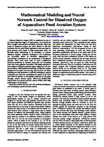
.Handbook of Intelligent Control. (ed. White and Sofge, 1992). Artificial neural networks can be used in several fields of control engineering: as process models, as controllers, for optimization and failure detection. Previous work (Garcia et al, 1986) refers to Model Predictive Control (MPC) as type of controllers in which there is a direct use of explicit and separate identifiable model. The same process model is implicitly used to compute the control action in such a way that the control design specifications are satisfied. Control design methods based on MPC concept have found wide acceptance in industrial applications due to their high performance and robustness. There are several variants of model predictive control methods, like Dynamic Matrix Control (DMC), Model Algorithmic Control (MAC) and Internal Model Control (IMC). Also nonlinear versions of these are developed, for example the nonlinear IMC concept. (Chen et al, 1994) A largely independently developed branch of MPC, called Generalized Predictive Control (GPC), is aimed more for adaptive control. For the current state-of-the-art of MPC (Clarke et al, 1989). For NNIMC, nevertheless, even though the NN model is available, it is complicated to design the NN inverse controller owing to the following reasons. First, the process required to be controlled, must be stable in open-loop, which certainly limits many of IMC applications (Saint-Donat et al., 1991; Willis et al., 1992). Second, the process to be controlled is required to have stable zero dynamics because of the use of the model inversion. For our understanding, little consequence has been reported about the NNIMC of nonlinear non affine discrete systems with unstable zero dynamics. Third, it may not be easy to have the model inversion for control law design due to the nonlinear internal model used. For the third problem mentioned previously, some solutions are introduced under certain conditions. One of the solutions is to train an NN inverse controller with the help of the identified NN model (Rumelhart et al., 1986, Baguman et al., 1990) If a nonlinear-in-the parameters type model is applied for adaptive control in a way analogical to the linear self-tuning scheme, one must accept that start-up behavior comparable to the linear case is not typically obtained and that all operation points should be visited at least once before good control performance is achieved. A minor off-line identification is of course a solution to the problems encountered during the initial start-up phase. This reduces the effect of randomly selected initial weights. (Rivals et al, 2000). The neural networks application in chemical engineering field offers potentially effective means of handling three difficult problems: Complexity, non linearity and uncertainties. The variety of available neural network architectures authorizes us to deal with a wide range of process control problems in comparison with other empirical models. Neural networks are relatively less sensitive to noise and incomplete information and deal with higher levels of uncertainty when applied in process control problems (Hunt et al., 1991). There are several results of research concerning the Neural Network – Internal Model Control (NN-IMC), which are implemented on different process (Rivals et al., 2000, Changjie et al., 2005, Varshney et al., 2009). These papers show that the advantages of Internal Model control systems are their robustness with respect to a model mismatch and to disturbances. In another paper, the NN-IMC was compared with conventional control (PID). It is shown that the NN-IMC has better performance than PID controller (Alarçïn, 2007). The objective of this paper is to obtain faster response performance in controlling binary distillation column using modified NN-IMC. The proper structure of NN model inverse and forward model, proper filter, and online training is needed. Multilayer feed forward neural networks with back propagation algorithm have been utilized for modeling in MATLAB and distillation column is modeled in HYSYS. Comparison of ANN based control schemes are illustrated using error analysis. 2. Distillation Column NN-IMC Control System 2.1 Distillation Column The column contains a total of NT theoretical trays. The liquid hold up on each tray including the down comer MN. The liquid on each tray is assumed to be perfectly mixed with composition XN, showing in Figure1, the mathematical formula expressing the process in the distillation column using rigorous modeling described as follows (Luyben, 1990): Nth tray Mass balance: dM N = L N +1 − L N + V N −1 − V N (1) dt Component mass balance: d( M N X N ) = L N +1 X N +1 − L N X N + V N −1Y N −1 − V N Y N dt

(2)

Energy balance: d( M N hN ) = L N +1 h N +1 − L N h N + V N −1 H N −1 − V N H N dt

(3)

179


Qc

VNT , YNT

AC xd

Condensor

rectifying L L F, X

,X N-1 N-1

Reflux drum

VN , YN

f

R = L /D LN , XN

V

Vb , Yb Lb , Xb

D

,Y N-1 N-1 AC xb

V stripping

D ,X

Qr reboiler V1

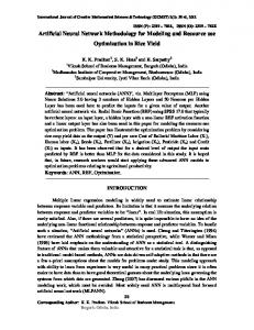
B , Xb Figure 1: Binary Distillation Column 2.2 Condenser and reflux drum The overhead vapor totally condensed in a condenser and flows into the reflux drum, whose holdup of liquid is MD (moles). The content of the drum is at its bubble point. Reflux is pumped back to the top tray (NT) of column at a rate L. Overhead distillate product is removed at a rate D Mass balance: dM D = V NT − L NT +1 − D (4) dt Component mass balance : d( M D X D ) = V NT Y NT − ( L NT +1 + D ) X D (5) dt Energy balance: d ( M D hD ) = V NT H NT − L NT +1 h NT +1 − DhD − Qc (6) dt 2.3 Reboiler and base column At the base of the column, liquid bottoms product is removed at a rate B and with composition XB. Vapor boil up is generated in thermosiphon reboiler at rate VB. Liquid circulates from the bottom of the column through the tubes in the vertical tube-in shell reboiler because of the smaller density of the vapor liquid mixture in the reboiler tubes. We will assume that the liquids in the reboiler and in the base of the column are perfectly mixed together and have the same composition XB and total holdup MB (moles). The composition of the vapor leaving the base of the column and entering tray 1st is yB. It is in equilibrium with the liquid with composition XB. Mass balance: dM N (7) = L1 − V B − B dt

180


Component mass balance: d( M B X B ) = L1 X 1 − V B YB − BX B dt

(8)

Energy balance: d ( M B hB ) = L1h1 − VB H B − BhB + QR dt

(9)

Feed tray (N = NF) A single feed stream is feed as saturated liquid onto the feed tray NF. Feed flow rate is F (mole/hour) and composition XF (mole fraction more volatile component). Mass balance: dM NF = L NF +1 − L NF + F + V NF −1 − V NF (10) dt Component mass balance: d ( M NF X NF ) = L NF +1 X NF +1 − L NF X NF + V NF −1Y NF −1 − V NF Y NF + Fz X F dt

(11)

Energy balance: d ( M NF h NF ) = L NF +1 h NF +1 − L NF h NF + V NF −1 H NF −1 − V NF H NF + Fh F dt

(12)

2.4 NN-IMC (Neural Network-Internal Model Control) The internal model control (IMC) scheme has been widely applied in the field of process control. This is due to its simple and straight forward controller design procedure as well as its good disturbance rejection capabilities and robustness properties. An Internal Model Control System (IMC) is presented in Figure 2. It consists of a collection of interconnected blocks: model, comparator, corrector, and controller. The model consist of controller model (Gc), plant model (Gp), forward model (Gm) and disturbance model (Gu). Basically in this structure, a feedback signal, result of a comparison between the actual process output Y and the model output of the process Ym to be controlled, is used to correct the reference signal (R). The feedback signal is active when a disturbance (U) acts on the process or the process and model behaviors are different. The IMC scheme has two interesting characteristics: • While modeling is accurately achieved, nominal tracking dynamic of the comprehensive system in absence of disturbance is reduced to that of the compensated process. The global system function is open loop. • Significant functioning is obtained even using a poor model. Generally, if the static gain of the compensated model is unity; full rejection of disturbance is achieved in steady state condition. U

Gu

R +

Gc

Gp

-

+ +

U1

C

Y -

Gm

+

Ym

Figure 2 : Neural Network IMC Structure The first characteristic implies that the process to be controlled must be stable. Accurate modeling of the process is not necessary thanks to the fairly significant robustness of the IMC scheme and approximate models of the process can often be satisfactory. Therefore a reduced amount of information about the process, such as the rise-time and the static gain, can be sufficient. Traditionally, internal models were implemented using mathematical equations. The structure of the model that was chosen could

181


use some previous knowledge of the plant, and the parameters obtained by an identification procedure. In some cases real time identification was used and the parameters of the model modified during the functioning of the system. The idea, here, is to use Internal Models implemented using NN in view of representing the knowledge of the control of the considered process. This is made possible because the internal model approach does not rely on an explicit mathematical model of the plant. Neural networks are information processing systems. Neural networks can be thought of as “black box” devices that accept input and produce output. Each neural network has at least two physical components: connections and processing element (neuron). The combination of these two components creates neural networks. In a broad sense, an artificial neural network diagram is consisting of three principal elements: • Topology – how a neural network is organized into layers and how those layers are connected. • Learning – how information is stored in the network. • Recall – how the stored information is retrieved from the network. In system identification view point, the advantages of neural networks to develop the model are nonlinear system, learning and adaptation, multivariable systems. Some of the most common neural networks are functional mapping nets like multilayer perceptron (MLP) and cerebellar model articulation computer (CMAC) (Albus,1975), adaptive resonance nets (ART) that form input categories from input data, input feature categorization nets of Kohonen (Kohonen,1984), bilinear associative memories and feedback network of analog neurons (Hopfield et al, 1985). An interpolation technique called Radial Basis Functions (RBF) (Moody, et al, 1989, Poggio et al 1990), is normally viewed as a neural network. Fuzzy models are also an efficient function approximation scheme. Multilayer perceptron (MLP) is one of the most commonly used neural network architecture today. It constructs an approximation of a multi-input multi-output function in a similar manner as fitting of a low order polynomial through a set of data points. A rich collection of different learning paradigms has been developed. Figure 3 illustrates the example of MLP networks, which consist of input, hidden and output layer. Input layer ϕd

Hidden layer f1 (• )

Output layer

F1 ( • )

ϕ2

F2 ( • )

ϕ1

y1

yC

f 2 (•)

w j,0

W k, 0

[w j, i ]

[W k,, j ]

Figure 3 : Structure of multilayer perceptron An important and useful feature of MLP networks is that the gradient and various other Jacobians of the model can be computed efficiently in a hierarchical and parallel manner using the chain rule differentiation. This gradient computation method is called the generalized delta rule or error back propagation. (Hopfield et al., 1985) This is commonly considered as a minimization method, i.e. it includes also the steepest descent parameter update. The terms forward pass and backward pass are used in this study to denote the computation of the predictions (forward) and the gradients (backward) only. Common nonlinear least squares methods are Levenberg-Marquardt (LM) and Gauss-Newton (GN) The MLP network is selected for the basic building block to be used in this study although localized representations have some useful properties over the MLP network. The learning algorithm using LM. The mathematical formula expressing what is going on in the MLP networks takes the form (Figure 3): ⎡ nh y k = F ⎢ Wk , j ⎢⎣ j =1

∑

⎤ ⎛ d ⎞ f⎜ w j ,i ϕ i + w j ,0 ⎟ + Wk ,0 ⎥ ⎜ ⎟ ⎥⎦ ⎝ i =1 ⎠

∑

k = 1,2,..C

(13)

All continuous function can be approximated to any desired accuracy with neural networks of one hidden layer of hyperbolic tangent hidden neuron and a layer of linear output neuron. (Clarke et al., 1989)

182


3. Design The first step of design: build the Amplitude Pseudo Random Binary Signal (APRBS), build the structure forward model of neural network for and inverse model of neural network from dynamic data of single distillation column binary system, choose low pass filter and tune gain controller to improve the performance of system. The second step: on-line training and choose an appropriate learning rate and an appropriate momentum in order to NN-IMC produce manipulated variable which make the control variable follow the set-point changes 3.1 Open loop data for training

xd (Fraction)

0.3 0.2 0.1 0

4 Qr (Kcal/min)

1

0 x 10

500 1000 t (Minute)

1500

0.9 0.85

8

2.4

3.5 3 2.5

0.95

L (gmol/min)

xb (Fraction)

0.4

0

500 1000 t (Minute)

1500

0 x 10

500 1000 t (Minute)

1500

500 1000 t (Minute)

1500

4

2.2 2 1.8

0

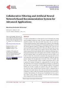
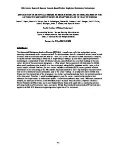
Figure 4 : Open loop data set for training The distillation column operated in open loop condition (inventory control only) in order to obtain its dynamic properties (Xd and Xb). Reflux (L) and steam reboiler (Qr) regulated according to signal APRBS (Amplitude Pseudo Random Binary Signal). Figure 4 shows the open loop - data which collected and they plotted against time. 3.2 Training of the forward model Forward model of distillation column is built using NN Multi layer Percepton (MLP), with input structure Neural Network AutoRegresive (NNARX), which trained by a couple of L and Qr as input-data and a couple Xd and Xb as output data and by using Levenberg Marquard as learning algorithm. (Figure 4.)

183


Input layer

Hidden layer

Output layer

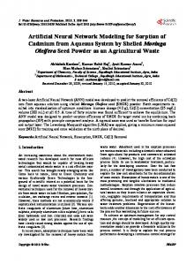
Figure 5 : NN forward model architecture Based on RMSE during training and validation phase, NN- forward model with 6 history lengths (HL) and 13 hidden nodes (HN) is chosen as the best NN structure (Figure 5). As shown in Figure 6 and 7, The RMSE are 5,9908 x 10-5 and 1,2686 x 10-4 for mole fraction of distillate (Xd) and mole fraction of bottom (Xb), respectively.

Figure 6 : Xd form process and NN model.

184


Figure 7 : Xb form process and NN model 3.3 Training the inverse model Similar procedure is applied to train the neural network - inverse model, as well as to train the forward model. The difference is on the inputs-model and on the outputs -model. Inputs of inverse model are Xd and Xb and its outputs are L and Qr, which obtained from training previously. Distillation column data which fed to the model are the past-data and the present-data.

Figure 8 : NN inverse model structure without disturbance input

Figure 9 : NN inverse model structure with disturbance input Figure 8 is inverse model structure without disturbance input (conventional inverse model) and Figure 9 is inverse model structure with disturbance input (modified inverse model). Both of inverse model of distillation column built-up from NN with

185


Multi layer Preceptor (MLP), Neural Network Auto Regressive, external input structure (NNARX), which trained by L and Qr as output data and Xd and Xb as input data (F and Xf constant and will update at online training) and by using Levenberg Marquard learning algorithm.

Figure 10 : Inverse model validation NN inverse model has 6 history lengths and 13 hidden nodes and trained for 200 times computer iteration is the best ANN structure to produce good RMSE. Two type NN inverse model have Root Mean Square Error (RMSE) about 0.0483 for L and RMSE about 0.0829 for the Qr. (Figure 10) 3.4 On Line Training The IMC control strategy required the inverse model as well as the forward model. IMC uses the forward model to compare with the process output and the deviation is used as one of the input to the inverse model (controller) to produce the better control action. IMC make use of both the inverse and forward model to predict the required control action input to the process. The IMC control strategy incorporates compensation to the inverse model because the output from the system is constantly being comparing with the output of the forward model. Figure 11 shows the control strategy for the Internal Model Control (IMC). +

E2

R ef

+

+ -

e

+ Inverse M odel

U

Y

P lant

+ + P lant

+

+

Y hat

E1

U = controller output / plant input Y hat = N N output Y = plant output ref = set point

e = error (Y -R ef) E 1 = error betw een plant and m odel E 2 = error betw een ref dn E 1

Figure 11 : Online training

186


The fact the inverse model is a recursive network is ignored during training in the sense that regresor’s dependency on the weights in the network is ignored. The simple training algorithm, which appears in accordance with this approximation, in some sense follows the spirit of so-called recursive pseudo-linier regression methods (PLR). 3.5 Filter The schematic diagram of NN-IMC for controlling binary distillation column is shown in Figure 12. Low pas filter had been used in this research is chosen by trial and error to filtered high frequency signal and adjusting the controller sensitivity. The filter transfer functions are: 3 1 Filter 2 = Fiter1 = s + 0.297229 s + 0,297229 4. Results and discussions Both of the proposed NN-IMC structure (conventional and modified) are stable and no error steady state. Proposed NN-IMC with inverse model input content of disturbance signal (modified NN-IMC) has better performance compare to NN-IMC without inverse model input content of disturbance signal. Proposed NN-IMC with disturbance input could get information about disturbance changing direct form measurement, so could produce manipulated variable signal early. The result has shown that process variable performance such as Integral Absolute Error (IAE) and settling time getting better. F & Xf

Disturbance

Ref(Xd & Xb )

+ Filter 1

+

JST Adaptif KOntroler

Filter 2

Proses

+

-

+ JST Forward Model

Ref = set point F = feed flow rate Xf = feed mole frac Xb = bottom mole frac

-

Xd = distilat mole frac C = control variable

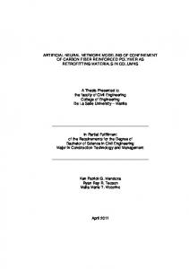
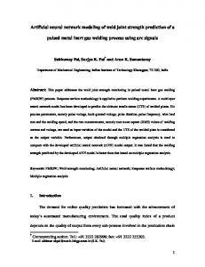
Figure 12 : NN-IMC for controlling binary distillation column Figure 13 shown that Xd response to the set point of Xd changes has rise time 187 minute and IAE 2.586 for NN-IMC structure with disturbance input and rise time 403 minute and IAE 4.4519 for NN-IMC structure without disturbance input. Figure 14 shown result of disturbance F change (increase from 45000 to 45450 gram mole/minute) that trajectory of Xd response return to the original set point at 266 minute and IAE 1.8133 for NN-IMC structure with disturbance input. Trajectory of Xd response return to the original set point at 500 minute and IAE 3.1608 for NN-IMC structure without disturbance input. set point

IMC Modified

IMC JST

0.9912

0.991

% metanol

0.9908

0.9906

0.9904

0.9902

0.99

0.9898 0

50

100

150

200

250

300

350

400

450

500

waktu(menit)

Figure 13 : Response Xd proposed NN-IMC when set point Xd changes.


187

set point

IMC Modified

IMC JST

0.99010

0.99000

% metanol

0.98990

0.98980

0.98970

0.98960

0.98950

0.98940 0

50

100

150

200

250

300

350

400

450

500

waktu(menit)

Figure 14 : Response Xd propose NN-IMC when disturbance F increase

Set Point

No

Table 1 : IAE for set point changes IAE NN-IMC With dist. input Xd Xb

IAE NN-IMC Without dist. Input Xd Xb 4.4519

1

(t=500 minute) Xd +0.001

2

Xd -0.001

3

Xb +0.001

2.1026

2.3046

4

Xb -0.001

2.1151

2.3575

2.5860 3.0235

5.0419

Table 1 shown IAE performance for set point changes and Table 2 shown IAE performance for disturbance changes. From the tables NN-IMC with disturbance input has better performance (IAE) than NN-IMC without disturbance input. Table 2 : IAE for disturbance changes No

IAE NN-IMC With dist. input

Disturbance

IAE NN-IMC Without dist. input Xd Xb

(t=500 minute)

Xd

Xb

1

F+1%

1.8133

11.0866

3.1608

12.8595

2

F-1%

1.8144

13.0649

3.1555

16.2314

3

Xf+1%

1.3694

12.9935

5.6888

23.4960

4

Xf-1%

1.4605

17.3190

5.5988

35.0071

5. Conclusions A forward model and two types of inverse models of binary distillation column have been built using NNARX. The models showed satisfactory performances as evidenced by the lower RMSE values of 5,9908 x 10-5and 1,2686 x 10-4 for mole fraction of distillate (Xd) and mole fraction of bottom (Xb), respectively. The RMSE of two types of inverse models have RMSE of about 0.0483 and 0.0829 for L and Qr, respectively. The models are therefore, ready to use in conventional and modified NN-IMC. Appropriate filters were selected and placed before and after the inverse model. Online training is also required for NN-IMC to obtain a better response in the system for controlling the binary distillation column. The simulation results, both conventional and modified NN-IMC have been found satisfactory. The proposed conventional and modified NN-IMC structures were found to be stable and no error steady state. This is mainly due to the selection of proper open loop data, optimized structure, proper filter, and adaptive inverse model. The inverse model with disturbance signal as input (modified NN-IMC) showed better performances in terms of lower IAE value and faster response as compared with the conventional NN-IMC. Future work will focus on the application of the proposed controller in many plants with difference complexities and characteristics. Acknowledgement Titik budiati would like to thank to Universiti Sain Malaysia and USM fellowship

188


References Alarçïn, F., 2007. Internal model control using neural network for ship roll stabilization, Journal of Marine Science and Technology, Vol. 15, No. 2, pp. 141-147. Albus, J. S., A New Approach to Manipulator Control. 1975. The Cerebellar Model Articulation Controller (CMAC). Trans. of the ASME. Journal of Dynamic Systems, Measurement and Control. Sept. 1975, pp. 220-227. Baguman, D.R. and Y.A Liu, 1990. Neural Networks in Bioprocessing and Chemical Engineering. Academic Press, San Dugo. Changjie Y., Jihong Z., and Zengqi S., 2005, Adaptive Neural Network Internal Model Control for Tilt Rotor Aircraft Platform, ICNC 2005, LNCS 3611, Springer-Verlag Berlin Heidelberg, pp. 262 – 265. Chen, Q. and W. A. Weigand. 1994. Dynamic Optimization of Nonlinear Processes by Combining Neural Net Model with UDMC. AIChE Journal, Sep. 1994, Vol. 40, No. 9, pp. 1488-1497. Clarke, D. W. and Mohtadi C., 1989. Properties of generalized predictive control. Automatica. Vol. 25, No. 6, pp. 859-875. Garcia, C. E., D. M. Prett, M. Morari, 1986, Model Predictive Control: Theory and Practice - a Survey. Automatica, Vol. 25, No. 3, pp. 335-348. Hernandez, E., Y. Arkun. 1992. Study of the control-relevant properties of backpropagation neural network models of nonlinear dynamical systems. Computers Chem. Eng, Vol. 16 No. 4, pp. 227-240. Hopfield, J. J., D. W. Tank. 1985. Neural. Computation of Decisions in Optimization Problems. Biol. Cybern, 52, pp. 141-152. Hunt, K. J.and Sbarbaro, D., 1991. Neural Networks for nonlinear internal model control, Proc. IEEE-Control Theory and Applications, Vol. 138, no. 5, pp. 431–438, Sep. Kanthasamy, R., 2009, Nonlinear model predictive control of a distillation column using hammerstein model and nonlinear autoregressive model with exogenous input, Thesis, Universiti Sains Malaysia Kohonen, T. 1984. Self-Organization and Associative Memory. Springer-Verlag, Berlin,.. Luyben, W.L., Process Modeling, Simulation, and Control for Chemical Engineers, McGraw-Hill Inc. Singapore, 1990. Moody, J., J. Darken. 1989. Fast learning in networks of locally-tuned processing units. Neural Computation, Vol. 1, pp. 281-294. Poggio, T., Girosi F. 1990. Regularization algorithms for learning that are equivalent to multilayer networks. Science, Vol. 247, pp. 978-982. Rivals, I. and Personnaz L., 2000. Nonlinear internal model control using neural networks: Application to processes with delay and design issues, IEEE Trans. Neural Netw., Vol. 11, No. 1, pp. 80–90. Rumelhart, D. E., Hinton G. E., Williams R. J. 1986. Learning internal representation by error backpropagation. In Rumelhart and McClelland [116], Vol. 1, Chapter 8. Saint-Donat, J., N. Bhat, T. J. McAvoy. 1991. Neural net based model predictive control. Int. J. Control, Vol. 54, No. 6, pp. 14531468. Qin,S.J., Badgwell, T.A, 2003, A survey of industrial model predictive control technology, Control Engineering Practice Vol. 11, pp. 733–764. Skogestad S. and Lundström, P., 1990, Mu-optimal LV-control of distillation columns, Computers & Chemical Engineering, Vol. 14, No. 4-5, pp 401-413. Varshney, T., Varshney, R., Sheel, S.,2009, ANN based IMC scheme for CSTR, International Conference on Advances in Computing, Communication and Control (ICAC3’09), pp 543-546. Willis, M. J., G. A. Montague et al. 1992. Artificial neural networks in process estimation and control. Automatica, Vol. 28, No. 6, pp. 1181-1187. Biographical notes Totok R. Biyanto is a lecturer in Engineering Physics Department – Industrial Technology Faculty, ITS Surabaya, He has published several papers in various national, international conferences and journals. He has an experience of 15 years as an instrumentation and process control consultant for many industries. Currently working at research & innovation office Universiti Teknologi Petronas, Malaysia. Titik Budiati is PhD student in School of Industrial Technology, Universiti Sains Malaysia. The scientific field is mathematical modelling. Bambang L. Widjiantoro is currently lecturer and Head of the Department of Engineering Physics, Sepuluh Nopember Institute of Technology (ITS) Surabaya, Indonesia. His research area is model predictive control, neural network based control system and process control. Ayman Abo Jabal received his M.Sc. degree from Czech Technical University Faculty of Technology Zlin in Plastic, Rubber and Leather Technology in 1996. Currently working in the Faculty of Engineering Industrial Technology Department at Sudan University of Science and Technology, His research interests are synthesis polymers material and composite, Rheological property data of Polymer Systems, kinetic reaction for formation and activation energy, thermodynamics.

Received July 2010 Accepted October 2010 Final acceptance in revised form November 2010