Missing:
Artificial Neural Network Based Prosody Models for Finnish Text-to-Speech Synthesis
Martti Vainio
University of Helsinki Department of Phonetics
Artificial Neural Network Based Prosody Models for Finnish Text-toSpeech Synthesis
Artificial Neural Network Based Prosody Models for Finnish Text-to-Speech Synthesis
Martti Vainio
University of Helsinki Department of Phonetics
Department of Phonetics University of Helsinki P.O. Box 35 (Vironkatu 1 B) FIN-00014, University of Helsinki, Finland ISSN 0357-5217 ISBN 952-10-0252-2 (Print) ISBN 952-10-0257-3 (PDF) Yliopistopaino c 2001 Martti Vainio Copyright
P¨aiville
ABSTRACT This thesis presents a series of experiments conducted on Finnish prosody for text-to-speech synthesis using artificial neural networks. The study serves the purpose of mapping and extracting out the relevant factors that have an effect on prosody in general – be they phonetic or linguistic in nature. The interplay between the relevant factors and the behavior of the prosodic parameters range from the simplest, phonetically determined variation on the segmental level to the linguistically determined variation on the level of the utterance. The fundamental idea of this work is to use similar models for all aspects and levels of suprasegmental and segmental prosodic phenomena – in effect building a superpositional and modular model from similar building blocks. All in all, a framework that can be further extended to encompass all levels of prosody is presented. Since the models are intended to work on all aspects and parameters of prosody, any underlying models that are generally used for prosody control in speech synthesis systems have been intentionally left out. That is, by allowing a large amount of redundancy in the models, the conceptual and practical discrepancy between, say, a tone sequence intonation model and a CART-based duration model has been circumvented. Nevertheless, it is not claimed that in a real world situation these models would out-perform a less redundant but more heterogeneous set of models. Instead, a conceptual framework that can be tailored to suit arbitrarily large domains and to include separate models for all aspects and scopes of prosody is presented. As mentioned, these models have not only intended for prosody control, but also to extract the relevant factors for each type of network – or each problem the network is intended to solve. That is, the presented artificial
x
Abstract
neural network methodology can be used to measure separate influences that the different phonetic and linguistic factors have on the complicated interplay among the physical prosodic parameters.
PREFACE Prosody modeling of Finnish has been basically non-existent for the period between the 1970’s (where it briefly existed) and the occurrence of the work presented in this thesis. Moreover, the basic methodology for doing such work has not been taught in Finnish universities – that is, how to bring together phonetic, linguistic and mathematical methods and knowledge that are necessary for such work. The research community has benefited from the good descriptive accounts of Finnish prosody that have existed for decades, and the Finnish scientific community has gained international fame with work on linguistic morphology on the one hand and neural computation on the other. But not until 1991, when Matti Karjalainen and Toomas Altosaar at the Helsinki University of Technology produced their first study on segmental duration modeling with artificial neural networks (ANNs), were these disciplines brought forward in a unified study. The study conducted by Karjalainen and Altosaar was a pioneering work in prosody modeling and this thesis builds on their results. This thesis is based on a collection of seven articles which were published between 1996 and 2000. The articles have a certain amount of overlap and it should be sufficient for the general reader to get acquainted with the introduction alone. The intended, or primary audience of this thesis is the future research worker who will be responsible to further push forward the prosody modeling for Finnish. It can be safely said that this work constitutes the majority of prosody modeling that has been conducted for Finnish, and that all further research and publications thereof on the subject are more than welcome. For the above reasons and to the benefit of the average reader, two somewhat superficial chapters have been included to this thesis. They deal with
xii
Preface
prosody modeling in general and Finnish prosody. More detailed information on both of these subjects can be found throughout the literature dealing with prosody and speech technology. Nevertheless, I hope that they will make this thesis more coherent and easier to follow. This is not an apology and if the reader perceives a sense of urgency in this work, he or she is not mistaken since models for Finnish prosody and their description are long overdue.
ACKNOWLEDGEMENTS I would like to thank the following institutions and people for providing me with the possibility to conduct the research presented here: The Academy of Finland, the University of Helsinki and the Alfred Kordelin fund for providing financial support: Professor Antti Iivonen for providing an unrestrained research environment at the Department of Phonetics as well as Professor Matti Karjalainen for doing the same at the Acoustics Laboratory of the Helsinki University of Technology; Professors Wim van Dommelen and Unto Laine for shining a harsh but necessary light on the first version of this manuscript; my colleagues and fellow research workers Stefan Werner, Reijo Aulanko and, especially, Toomas Altosaar, who has influenced my work on so many levels – positively, of course. I would also like to thank the members of my family in which I grew up – especially my father and mother without whom none of this would exist. And above all, I thank the members of my family with whom I share the daily life; your love and patience have been the basic requisite for this work!
xiv
Acknowledgements
CONTENTS
Abstract . . . . . . . . . . . . . . . . . . . . . . . . . . . . . . . . . . .
ix
Preface . . . . . . . . . . . . . . . . . . . . . . . . . . . . . . . . . . .
xi
Acknowledgements . . . . . . . . . . . . . . . . . . . . . . . . . . . . . xiii List of Figures . . . . . . . . . . . . . . . . . . . . . . . . . . . . . . . xix List of Tables . . . . . . . . . . . . . . . . . . . . . . . . . . . . . . . . xxi List of Abbreviations . . . . . . . . . . . . . . . . . . . . . . . . . . . . xxiii List of Publications . . . . . . . . . . . . . . . . . . . . . . . . . . . . . xxv 1. Introduction . . . . . . . . . . . . . . . . . . . . . . . 1.1 Overview . . . . . . . . . . . . . . . . . . . . . . 1.2 Prosody Modeling and Text-to-Speech Synthesis 1.2.1 Data-based models . . . . . . . . . . . . 1.3 Organization of this Thesis . . . . . . . . . . . . 1.4 Author’s Involvement in the Published Work . .
. . . . . .
. . . . . .
. . . . . .
. . . . . .
. . . . . .
. . . . . .
. . . . . .
2. An Overview of Existing Models for Prosody . . . . . . . . . . . . 2.1 Segmental Duration Models . . . . . . . . . . . . . . . . . . 2.1.1 Klatt Rules . . . . . . . . . . . . . . . . . . . . . . . 2.1.2 Linear Statistical Models – Sums-of-Products Model . 2.1.3 Classification and Regression Trees (CART) . . . . . 2.1.4 Syllable Durations with Neural Networks . . . . . . .
. . . . . .
1 1 2 2 4 5
. 7 . 8 . 8 . 9 . 10 . 12
xvi
Contents
2.2 Intonation Models . . . . . . . 2.2.1 Tone Sequence Models 2.2.2 Fujisaki Model . . . . 2.2.3 Tilt Intonation Model 2.3 Prosody Modeling for Finnish 3. Finnish Prosody and Domains 3.1 Lexical Prosody . . . . . 3.2 Segmental Prosody . . . 3.3 Sentence Level Prosody .
. . . . .
. . . . .
. . . . .
. . . . .
. . . . .
. . . . .
. . . . .
. . . . .
. . . . .
. . . . .
. . . . .
. . . . .
. . . . .
. . . . .
. . . . .
. . . . .
. . . . .
. . . . .
13 16 17 18 20
of Modeling . . . . . . . . . . . . . . . . . . . . .
. . . .
. . . .
. . . .
. . . .
. . . .
. . . .
. . . .
. . . .
. . . .
. . . .
. . . .
. . . .
. . . .
. . . .
23 26 27 29
4. Data . . . . . . . . . . . . . . . . . . . . . . . . . . . . . . . . . . . 33 4.1 Segmental and Lexical Level Experiments . . . . . . . . . . . 34 4.2 Sentence Level Intonation and Morphological Experiments . . 36 5. Methods . . . . . . . . . . . . . . . . . . . . . . . . . . . 5.1 A Short Introduction to Artificial Neural Networks 5.1.1 Artificial Neuron . . . . . . . . . . . . . . . 5.1.2 Network Architecture . . . . . . . . . . . . . 5.1.3 Learning in Neural Networks . . . . . . . . . 5.1.4 Pre- and Post-processing . . . . . . . . . . . 5.1.5 Feature Selection . . . . . . . . . . . . . . . 5.2 Neural Network Methodology Used in this Research 5.2.1 Input Coding . . . . . . . . . . . . . . . . . 5.2.2 Output Coding . . . . . . . . . . . . . . . .
. . . . . . . . . .
. . . . . . . . . .
. . . . . . . . . .
. . . . . . . . . .
. . . . . . . . . .
. . . . . . . . . .
39 39 40 42 42 43 44 45 48 52
6. Results . . . . . . . . . . . . . . . . . . . . . . . . . . . . . . . 6.1 Segmental Prosody . . . . . . . . . . . . . . . . . . . . . 6.2 Word Level Prosody . . . . . . . . . . . . . . . . . . . . 6.2.1 Specialization . . . . . . . . . . . . . . . . . . . . 6.2.2 Effect of Context Size . . . . . . . . . . . . . . . 6.2.3 Relative Importance of Different Input Factors . . 6.3 Sentence Level Prosody . . . . . . . . . . . . . . . . . . . 6.3.1 Influence of Morphology on Network Performance
. . . . . . . .
. . . . . . . .
. . . . . . . .
55 56 60 60 62 64 65 66
Contents
xvii
6.3.2
Modeling Accuracy . . . . . . . . . . . . . . . . . . . . 68
7. Conclusion . . . . . . . . . . . . . . . . . . . . . . . . . . . . . . . . 77 7.1 Future Work . . . . . . . . . . . . . . . . . . . . . . . . . . . . 80 A. Database Labeling Criteria . . . . . . . . . . . . . . . . A.1 Summary of Speech Database Labeling Criteria . A.1.1 Utterance Boundary . . . . . . . . . . . . A.1.2 Segment Boundaries within Utterances . . A.2 Statistical Analyses of Segmental Durations . . . A.3 Distribution of Words According to Part-of-speech
. . . . . .
. . . . . .
. . . . . .
. . . . . .
. . . . . .
. . . . . .
. . . . . .
83 83 84 84 95 98
xviii
Contents
LIST OF FIGURES 2.1 2.2 2.3 2.4 2.5
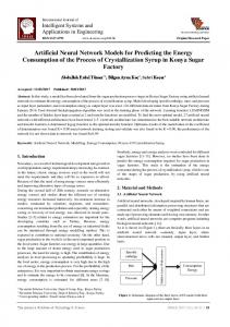
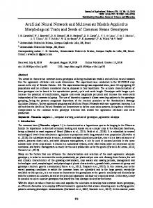
A partial decision tree for segmental durations. . A comparison of intonation models. . . . . . . . . An example sentence analyzed the Fujisaki model. The Tilt intonation model. . . . . . . . . . . . . . Matti Karjalainen’s intonation model for Finnish.
. . . . .
. . . . .
. . . . .
. . . . .
. . . . .
. . . . .
. . . . .
11 15 19 20 21
3.1 3.2 3.3 3.4
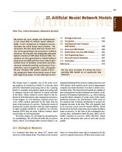
Sentence “Tarkka kirurgi varoo n¨ak¨oa¨a¨n”. . . . . . . . . . The stress structure for the phrase “Jyv¨askyl¨an asemalla”. The word “sikaa”. . . . . . . . . . . . . . . . . . . . . . . . The word “aamunkoitossa”. . . . . . . . . . . . . . . . . .
. . . .
. . . .
25 26 29 31
4.1 Distribution of sentence durations in the corpus. . . . . . . . . 35 4.2 A waveform and spectrogram of a typical Finnish utterance. . 37 5.1 5.2 5.3 5.4 5.5 5.6 5.7 5.8
An artificial neuron as found in most multi-layer perceptrons. The logistic (sigmoid) function. . . . . . . . . . . . . . . . . . Pre- and post-processing of data for neural networks. . . . . . A global view of the model for prosody control proposed in this study. . . . . . . . . . . . . . . . . . . . . . . . . . . . . . Neural network architecture. . . . . . . . . . . . . . . . . . . . Representation of phonetic context. . . . . . . . . . . . . . . . Spatial coding for phonetic context. . . . . . . . . . . . . . . . Duration distributions for training data. . . . . . . . . . . . .
40 41 44 45 47 49 51 53
6.1 Examples of F 0 networks’ results. . . . . . . . . . . . . . . . . 58 6.2 Error percentages for lexical level duration networks. . . . . . 61 6.3 Average absolute relative errors for the duration networks. . . 63
xx
List of Figures
6.4 Averaged values for different factors’ effect on network performance. . . . . . . . . . . . . . . . . . . . . . . . . . . . . . . 6.5 Actual vs. predicted contours, example 1. . . . . . . . . . . 6.6 Actual vs. predicted contours, example 2. . . . . . . . . . . 6.7 Actual vs. predicted contours, example 3. . . . . . . . . . . 6.8 Segmental duration predictions vs. observed values. . . . . . 6.9 Observed vs. predicted pitch. . . . . . . . . . . . . . . . . . 6.10 Duration prediction error vs. expected duration . . . . . . . 6.11 Pitch prediction error vs. expected pitch. . . . . . . . . . . .
. . . . . . . .
65 68 69 70 72 73 74 75
A.1 A.2 A.3 A.4 A.5
. . . . .
86 87 89 91 92
Segmentation Segmentation Segmentation Segmentation Segmentation
of of of of of
a a a a a
vowel-fricative pair. . . . . stop-vowel, vowel-vowel and nasal-fricative pair. . . . . . vowel-liquid pair. . . . . . . trill-vowel pair. . . . . . . .
. . . . . . . vowel-stop. . . . . . . . . . . . . . . . . . . . . .
. . . . .
LIST OF TABLES 4.1 Contents of the Finnish Speech Database . . . . . . . . . . . . 34 5.1 Morphological factors as network input. . . . . . . . . . . . . . 50 5.2 Miscellaneous word-level input information . . . . . . . . . . . 50 6.1 Segmental level network estimation results. . . . . . . . . . . . 59 6.2 Results from adding morphological information, function word and part-of-speech information to the network input. . . . . . 67 A.1 Duration data for the phones in the 692-sentence database. . . A.2 Average z-scores of syllables according to the position in word. A.3 Average z-scores of the word-initial syllables according to the type of word. . . . . . . . . . . . . . . . . . . . . . . . . . . . A.4 Average z-scores for utterance final, penultimate and antepenultimate syllables. . . . . . . . . . . . . . . . . . . . . . . . A.5 Average z-scores for utterance final and penultimate as well as other than final phones. . . . . . . . . . . . . . . . . . . . . A.6 Average z-scores for utterance final, penultimate and antepenultimate words. . . . . . . . . . . . . . . . . . . . . . . . . A.7 Distribution of words according to part-of-speech. . . . . . . .
94 96 96 97 97 98 98
xxii
List of Tables
LIST OF ABBREVIATIONS ANN C CART DUR EBP F0 INHDUR JND MINDUR MLR MLP o SOM t TTS HMM V
Artificial Neural Network Consonant Classification and Regression Tree Segmental duration Error back-propagation Voice fundamental frequency Inherent duration of a segment Just noticeable difference Minimal duration of a segment Multiple Linear Regression Multi-layer perceptron Network Output Self Organizing Map Network Target Text-to-Speech Hidden-Markov Model Vowel
xxiv
List of Abbreviations
LIST OF PUBLICATIONS 1. Martti Vainio and Toomas Altosaar. Pitch, loudness, and segmental duration correlates: Towards a model for the phonetic aspects of Finnish prosody. In H. Timothy Bunnell and William Idsardi, editors, Proceedings of ICSLP 96, volume 3, pages 2052–2055, Philadelphia, 1996. 2. Martti Vainio and Toomas Altosaar. Pitch, Loudness and Segmental Duration Correlates in Finnish Prosody. In Stefan Werner, editor, Nordic Prosody, Proceedings of the VIIth Conference, Joensuu 1996, pages 247 – 255. Peter Lang, 1998. 3. Martti Vainio, Toomas Altosaar, Matti Karjalainen, and Reijo Aulanko. Modeling Finnish Microprosody for Speech Synthesis. In Antonis Botinis, Georgios Kouroupetroglou, and George Carayannis, editors, ESCA Workshop on Intonation: Theory, Models and Applications, September 18-20, 1997, Athens, Greece, pages 309 – 312. ESCA, University of Athens, 1997. 4. Matti Karjalainen, Toomas Altosaar, and Martti Vainio. Speech synthesis using warped linear prediction and neural networks. In Proc. IEEE Int. Conf. Acoustics, Speech, and Signal Processing (ICASSP’98), pages 877 – 880, 1998. 5. Martti Vainio and Toomas Altosaar. Modeling the microprosody of pitch and loudness for speech synthesis with neural networks. In Proceedings of ICSLP 98, Sydney, 1998. 6. Martti Vainio, Toomas Altosaar, Matti Karjalainen, Reijo
xxvi
List of Publications
Aulanko, and Stefan Werner. Neural network models for Finnish prosody. In John J. Ohala, Yoko Hasegawa, Manjari Ohala, Daniel Granville, and Ashlee C. Bailey, editors, Proceedings of the XIVth Internation Congress of Phonetic Sciences, pages 2347 – 2350, 1999. 7. Martti Vainio, Toomas Altosaar, and Stefan Werner. Measuring the importance of morphological information for Finnish speech synthesis. In Baezon Yuan, Taiyi Huang, and Xiaofang Tang, editors, Proc. ICSLP 2000, volume 1, pages 641–644, Beijing, China, October 2000.
Chapter 1 INTRODUCTION
1.1 Overview This chapter will give a brief description of the contents and the structure of this thesis as well as a slightly more lengthy discussion about problems associated with prosody modeling and text-to-speech synthesis (TTS) in general. The basic problem motivating this study was the lack of prosody models for Finnish. Such models are necessary in many respects: first of all, they are an essential part of any high quality TTS system and secondly, they provide a framework for the description of the phenomena that prosody comprises. The general problems with prosody modeling lie in the grey area between the discrete, symbolic representation of speech and its actual manifestation as a continuously varying signal. Basically, one needs to develop a methodology to associate a set of linguistic, para-linguistic and emotional instructions or representations with the prosodic parameters of synthetic or natural speech. The solution to the above problems presented in this thesis is based on data, artificial neural networks (ANN), and the general methodology related to their use. The most significant results from this study are, firstly, that neural networks can be used for both prosody control in Finnish TTS and that they may be used so directly – there is no need for underlying models and, secondly, that the modeling paradigm presented here can be used for certain aspects of prosody research in general.
2
Chapter 1. Introduction
1.2 Prosody Modeling and Text-to-Speech Synthesis The essence of text-to-speech synthesis is to convert symbols into signals. Thus, a TTS system occupies a special place in the realm of information technologies. As the signal generation systems, i.e., the speech synthesizers themselves have moved into the domain of sampled speech and stored forms, the main problem of adding naturalness and intelligibility to the systems can largely be solved by incorporating better prosody models. The mapping from a string of phonemes or phones and the linguistic structures in which they participate, to the continuous prosodic parameters is a complex and nonlinear task. This mapping can, and has traditionally been done by sets of sequentially ordered rules which control a synthesizer that produces the digital forms of the signals that are then rendered audible by some means. Nevertheless, a set of rules cannot describe the nonlinear relations past a certain point without getting impractically large and complicated. The rules are usually as general as possible and exceptions to them tend to extend and complicate the rule-set. Moreover, rule development is usually based on the introspective capabilities and expertise of individual research workers. It usually reflects their theoretical backgrounds, which is only natural, but can be a burden if the theories rely too much on introspection and subjective measurements. 1.2.1 Data-based models In speech synthesis, data-based, statistical methods have practically replaced explicit rules. These modern data-oriented methods include Hidden Markov Models (HMM), Classification and Regression Trees (CART) and Artificial Neural Networks. The investigation of prosodic variation has a serious problem in common with the study of many other aspects of speech and language research; one frequently encounters phenomena that are both extremely common as well as extremely rare. (See for instance van Santen in [69] and [31].) This makes the preparation of representative databases for all speech phenomena and their combinations practically impossible even in a fairly constrained domain, such
1.2. Prosody Modeling and Text-to-Speech Synthesis
3
as prosody. The situation calls for models that can produce generalizations and accurately predict patterns that are absent in the data. Neural networks are known for their ability to generalize according to the similarity of their inputs but also to distinguish different outputs from input patterns that are similar only on the surface. As a consequence, networks have the power to predict, after an appropriate learning phase, even patterns they have never seen before. This provides the researcher with a potential solution to the problem of constructing models from imperfect data. The problem, then, boils down to finding an optimal network organization and data representation as well as a method for training the network successfully from real speech data. Provided, of course, that one has large amounts of high-quality speech data available.1 In this study neural networks were used to accomplish the prediction of continuous values for fundamental frequency, loudness and segmental duration, which in turn determine the accentuation and prominence level of the syllables and phones within the utterances. This is done for the same reason that most researchers use decision trees (see for instance [12], [23], [8] and [53]). That is, neural networks should in principle enjoy the same advantages the decision tree methodology does; “they can be automatically trained to learn different speaking styles and they can accommodate a range of inputs from simple text analysis for the problem of synthesis from unrestricted text to more detailed discourse information that may be available as a by-product of text generation” [12]. Moreover, artificial neural networks with hidden units can learn new features that combine multiple input features. This is also a drawback when the inner workings of a network are under study and one desires to learn more about the way the networks accomplish their task. The modeling framework presented here assumes the existence of a text
1
The data that are used to train speech synthesis systems have very stringent requirements concerning the segmentation and annotation (i.e., labeling) of the utterances. Since the amount of well-labeled data available is usually small compared to data used for training automatic speech recognizers, the requirements for the quality of the content of the data are also increased.
4
Chapter 1. Introduction
processing module that is capable of providing neural networks information about the linguistic structure of the text. At this point no explicit information or instructions in the form of intonational transcriptions have been used, but the networks rely on their ability to infer the necessary information from the input text and its implicit linguistic and phonetic structure. In other words, the training data contained no annotations for prosodic constituent structure. The models described here are, not like Taylor’s Tilt model [57] and Fujisaki’s superpositional intonation model [16], phonetic in nature. Their purpose is not only to describe observable linguistic sound phenomena [57], but to associate these phenomena with the abstract linguistic structures. The increasing scope of information and context in terms of hierarchical levels and horizontal extent described in this thesis could be used for a “proof by induction” for the case that neural network models could be extended to give representations to arbitrarily large domains; i.e., the problem of producing correct prosody can be divided into a) the problem of identifying the particular types of information that have an effect on physical parameters, and b) acquiring and labeling sufficient amounts of data for model training. As an example, one could imagine a situation where different types of information that have been identified by conversation analysis techniques could be coded as network input. Similarly, the givenness of each word could be easily added by simply making the networks aware of the occurrence of any given word (or a semantic feature that it shares) before and the distance of the word from the current one; any metric that can be translated to the network input space would do.
1.3 Organization of this Thesis The first chapter of this thesis gives an overview of the problems commonly encountered in prosody modeling as well some discussion about the relative merits of different modeling paradigms. The rest of the chapter describes the outline of this thesis and gives an account of the author’s contributions in relation to the published work.
1.4. Author’s Involvement in the Published Work
5
The second chapter gives an outline of some existing models used for prosody control in various TTS-systems. This chapter and the following one, which gives an account of Finnish prosody, are fairly shallow with respect to detail and are intended to give support the reader who comes from outside the field of prosody and speech technology. The fourth chapter gives a description of the various databases and the fifth chapter gives a short introduction to the neural network methodology used in this study. The results from the study are discussed in various degrees of detail in the sixth chapter. The final chapter serves as a conclusion to the thesis with a recapitulation of the actions taken, some concluding remarks about the results and a section on future directions of study.
1.4 Author’s Involvement in the Published Work The following is a brief summary of the publications (see Page xxv) and the author’s involvement in their preparation as well as the research work: • Paper 1 describes the basic methodology used for word level prosody modeling including the neural network architecture. Basic results from pitch, loudness and segmental duration as well as some error analyses are described. The author was the main researcher in the study and the final paper was mostly written by him. • Paper 2 is basically a continuation of paper 1 with results from new experiments relating to specialization. The paper also includes a description of a new methodology for evaluating the relative importance of different input factors and summarizes the results from experiments of word level data. The author was the main researcher in the study and also wrote the paper. • Paper 3 describes the extension of the methodology into modeling microprosodic variation. An alternative method based on multiple linear
6
Chapter 1. Introduction
regression (MLR) is also described. Results from both neural network and MLR modeling are presented. The author was the main researcher in the study and also wrote the paper. • Paper 4 describes the global structure of the synthesizer where the neural network models were intended to act as the prosody control module. The author was responsible for the section describing prosody control. • Paper 5 is a continuation of paper 3. New results for microprosody of both pitch and loudness are presented as well results from applying the methodology to sentence length material. The author was the main researcher in the study and also wrote the paper. • Paper 6 describes work done on both word level and segmental level prosody. New results from sentence level prosody are presented. The author was the main researcher in the study and also wrote the paper. • Paper 7 describes results from extending the models with linguistic information. Specifically, results from experiments to determine the relative importance of different levels of linguistic information for predicting segmental durations and syllabic pitch values are presented. The author was the main researcher in the study and also wrote the paper.
Chapter 2 AN OVERVIEW OF EXISTING MODELS FOR PROSODY Prosody is an elementary component in all text-to-speech systems. No system seriously attempts to produce the full range of phenomena that can be conveyed in speech with the means of varying fundamental frequency, intensity and timing, the main physical parameters used in prosody control in text-to-speech systems. Instead, most research is centered around producing a declarative reading – void of any emotion – of the input text (with the exception of providing different pitch contours for questions when necessary). Even this restricted goal is difficult to achieve with the current state of knowledge and technology. The models used for prosody control range from rule-based methods to trainable, data-based methods. The extreme ends of this continuum both have their merits as well as problems: rule-based models often generalize too much and cannot handle exceptions well without getting exceedingly complicated; data-based methods are generally dependent on the quality and quantity of available training data (see Chapter 1 and references therein for more detail about the scarcity-of-data problem). Although there are three acoustic parameters that need to be predicted, loudness is often either completely neglected or is modeled concurrently with fundamental frequency. This is based on the assumption that the loudness contour is implied by the fundamental frequency of the utterance. Many concatenative synthesizers based on either linear prediction or overlap-and-add methods (e.g., MBROLA [13]) use the inherent loudness values in the diphone data and no other modeling is used. Although, in the case of MBROLA, the possibility to control loudness is currently being studied.
8
Chapter 2. An Overview of Existing Models for Prosody
Thus, prosody control is usually accomplished with three separate modules: prosodic boundary placement, segmental duration determination and F 0 contour specification. Since the research presented here is mainly concerned with segmental durations and intonation1 , the rest of this chapter discusses some of the most influential existing models – those concerning loudness, pause insertion, and pause length prediction are ignored. The ones discussed here represent, of course, only a fraction of the prosody models in existence and were chosen because of their influence on TTS systems development and prosody research in general.
2.1 Segmental Duration Models Four distinct segmental duration models are introduced. They range from purely knowledge-oriented, rule-based models to purely data-based models which gain their predictive power directly from the data. 2.1.1 Klatt Rules Dennis Klatt proposed a rule-based system [41] which was implemented in the MITalk system [2]. His model was based on information presented in phonetic literature about the different factors affecting segmental duration. The duration of each phone was calculated according to the following equation:
DU R = (IN HDU R − M IN DU R) ∗
P RCN T + M IN DU R 100
(2.1)
where INHDUR and MINDUR are the inherent and minimum durations for the phone, respectively. PRCNT is the shortening in percent of the 1
In this thesis the term prosody is used for all suprasegmentals and intonation for the variations in fundamental frequency (usually and if not explicitly mentioned, on the level of sentence/utterance). Daniel Hirst and Albert Di Cristo give a good overview of the different definitions for the basic terminology and the consequent problems in [25].
2.1. Segmental Duration Models
9
duration change which is determined by the rules themselves. Klatt used ten rules that were based on effects of the phonetic environment, emphasis, stress level, etc. on the current phone’s duration. Each rule adjusts the PRCNT term in a multiplicative manner and the final result is the product of the rules plus the effect of one final rule that is applied after the calculation of DUR in equation 2.1 [2]. As with any rule-based models, the Klatt rules and their parameter values are determined manually by a trial-and-error process. 2.1.2 Linear Statistical Models – Sums-of-Products Model Jan van Santen has developed a model which seems to be able to address the scarcity-of-data problem better than other data-based models ([70], [71], [69] and [53]). His model is linear and is based on a collection of equations that are determined according to prior phonetic and phonological information as well as information collected by analyzing data. He calls it the sums-ofproducts model for the reason that each equation, which is determined by certain contextual factors, represents a sum of a sequence of products of terms associated with the contexts. Equation 2.2 shows a typical sums-ofproducts model whose variables have to be manually determined from data by standard least-squares methods.
DUR(Vowel:/e/, Next:V oiced, Loc:F inal) = α(/e/) + δ(F inal) + β(V oiced) × γ(F inal)
(2.2)
Equation 2.2 states that the duration of a vowel /e/ which is followed by a voiced consonant and is in utterance-final position is given by taking the intrinsic duration of the vowel [α(/e/)], adding a certain number of milliseconds for being utterance-final [δ(F inal)], and finally adding the effect of post-vocalic voicing [β(V oiced)] modulated by utterance-finality [γ(F inal)]. The model is based on the assumption that most factors that have an effect on segmental durations have the property of directional invariance; for instance, with other factors being constant, the stressed vowels are longer
10
Chapter 2. An Overview of Existing Models for Prosody
than non-stressed ones – i.e., the direction of the effects of a factor is unaffected by other factors. Van Santen makes the claim that sums-of-products models have the property that they can capture directionally invariant interactions using very few parameters [72]. The sums-of-products models are applied by constructing a tree whose terminal nodes split the feature space into homogeneous subclasses each of which is represented by a separate sums-of-products model. This is done manually by incorporating knowledge from literature and information from exploratory data analysis. 2.1.3 Classification and Regression Trees (CART) The Classification and Regression Trees are typical data-based duration models that can be constructed automatically. This capability of self-configuration makes them very popular; for instance the Festival speech synthesis system includes tools for building such trees from existing databases [7]. A duration predicting CART is basically a binary-branching tree whose inputs are instances of phones which are fed in from the top node. The phones then pass through the arcs satisfying their constraints. Figure 2.1 shows a partial tree constructed to determine segmental durations for Finnish. The numbers in the leaf-nodes are so called z-scores and the final durations are calculated according to an equation which states that duration = mean + (z-score * standard deviation). Both the mean and standard deviation are estimated from a corpus. The tree in Figure 2.1 has already satisfied the following criteria: the current phone is in a lexically unstressed syllable, it is the coda of the syllable and the syllable itself is fewer than three syllables from a following phrase break. The circles in the figure depict omitted sections. As an example, the tree asserts that the duration of the phone [u] in word [minut] is approximately 81 milliseconds (0.065 + (0.717 ∗ 0.022) = 0.080774 where 0.065 and 0.022 are the mean and standard deviation in milliseconds for [u] in the database.). The tree itself is constructed (or grown) with an algorithm that accepts sample phones with correct outputs, in this case their observed z-scores from
2.1. Segmental Duration Models
11
current phone is + voc, −long n
y
next is −voc
current phone is +voc, +round n
y
prev is +voc
y
next is +nas
y
n
y
0.003
−0.138
prev is +voc y −0.597
n
n −0.978
n
syllable dist. to pause < 2.5 next is +cons, +lab n y n y
1.398
0.115 next is +cons,+voc y 2.923
n 0.717
next is +cons, +voc y 0.872
n 0.519
Fig. 2.1: Partial decision tree for segmental durations in Finnish. The circles depict omitted sections.
a set of training data. Usually the tree-constructing methods look for a binary split that is 1) determined by a single factor and 2) that best correlates with the data. Basically, the algorithm clusters durations according to their contexts. Usually the contextual effects that are used include the stress level of the current phone, its position in the word, its position in the phrase, and the phonetic context within a window that spans a number of phones on either side of the current one. These are, of course, the basic factors that are known to influence segmental durations. The tree in Figure 2.1 was trained with a subset of the 1126-sentence corpus described in Chapter 4.
12
Chapter 2. An Overview of Existing Models for Prosody
Using individual phone identities in the description of the phonetic context usually leads to highly individual and distinct feature vectors and therefore increases their number. This usually leads to problems concerning the coverage of data that are difficult to address without gathering and labeling enormous amounts of speech for model training. Therefore, it is better to describe the context in terms of broad classes; i.e., the phones can be grouped according to their phonological features. This is how the problem is usually solved in data-based systems. The tree-constructing algorithms usually guarantee that the tree fits the training data well but there is no guarantee that new and unseen data will be properly modeled. The tree may simply be over-trained to fit the idiosyncrasies in the training data [46]. However, there is a way to get around this problem by pruning the tree by cutting off the branches that are responsible for the over-training. The pruning is usually done by evaluating the tree on some unseen data (usually called the pruning set) and then simplifying the tree by cutting off the parts that do not fit well to the pruning data. 2.1.4 Syllable Durations with Neural Networks Campbell [10] has devised a neural network based model which predicts syllable durations and then fits phone durations to the syllables. He uses neural networks because it is assumed that the networks can learn the underlying interactions between the contextual effects. That is, they should be able to represent the rule-governed behavior that is implicit in the data (this is precisely the reason for using them for all aspects of prosody modeling in this study). If the networks can code the underlying interactions, they should do well with unseen data. Campbell computed a feature vector for each syllable which consisted of information about the syllable’s length in terms of number of phones, the nature of the syllable nucleus (Campbell calls it the syllabic peak ), the position in tone-group, the type of foot, stress level, and word class (function vs. content word). He then predicted the syllable durations with these feature vectors and an artificial neural network. The phone durations within
2.2. Intonation Models
13
the predicted syllables were then determined by their elasticity. The elasticity is determined from a normalized duration which is calculated “by subtracting the means and expressing the residuals in terms of their standard deviations to yield a zero with unit variance for each phoneme distribution” [10]. These normalized values then represent the amount of lengthening or compression undergone by each segment relative to its elasticity. According to Campbell, in the majority of cases, the amount of compression or lengthening within a syllable can be expressed with a single constant which is determined from data by solving the following equation for k: n X
exp(µi + kσi )
i=1
The equation returns the duration for a syllable of length n in milliseconds (exponentiation is due to the fact that all durations in the system are expressed in logarithmic form (see section 5 for more detail)). The segment (i ) is assigned the duration according to exp(µi +kσi ) where µi and σi are the mean and standard deviation of the log-transformed duration for the realization of phone or phoneme class (e.g., [e]) represented by i. Some analyses of Finnish data done with this kind of normalization scheme can be found in Appendix A.
2.2 Intonation Models Two major schools for intonation modeling have emerged within the last twenty years: the tone sequence school which follows a traditional phonological description of intonation and the more phonetically oriented superposition school. The tone sequence models interpret the F 0 contour as a linear sequence of phonologically distinctive units (tones or pitch accents), which are local in nature. These events in the F 0 contour do not interact with each other and their occurrence within the sequence can be described by a grammar. That is, they are linguistic in nature. The most influential of the models is based on Janet Pierrehumbert’s theory, which was presented in her doctoral thesis
14
Chapter 2. An Overview of Existing Models for Prosody
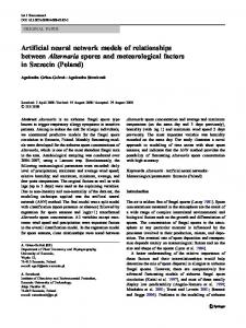
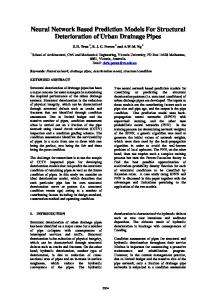
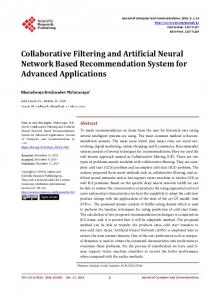
in 1980 [50] and led to a widely used and popular transcription system ToBI (Tone and Break Indices [52]). On the other end of the continuum are the superpositional models which are phonetic in nature. They are hierarchically organized models which interpret the F 0 contour as a complicated pattern of components that are superimposed on each other. The best known of these models is the Fujisaki ¨ model [15] which was inspired by theories developed by Ohman in the sixties [27]. The main difference between these models is how local movements (e.g., accents) and global phenomena (e.g., declination) and their relations are viewed. The problem, of course, is that all those phenomena are manifested in the same signal; basically the F 0 contour (although the amount of influence loudness, segmental durations and other factors have on the perception of these phenomena is not well known – this is problematic especially with the tone sequence models as they usually depend on human produced transcriptions). The basic problem with intonation models in general is how to separate accentuation from intonation 2, [48]; that is, the word-level phenomena from the more global, sentence-level phenomena. This cannot be achieved on the acoustic basis alone; a linguistic description is needed. One should be able to formulate a set of “rules that can predict accent- or intonation-related patterns independent of, as well as in interaction, with each other” [48]. On the basis of this argument, none of the current models can and should be purely phonological as opposed to phonetic. Figure 2.2 shows a comparison of four different intonation models ranging from Pierrehumbert’s tone sequence model to Paul Taylor’s Tilt model. The Pierrehumbert model, inevitably, belongs to the tone sequence school; Fujisaki’s model is the quintessential superpositional model whereas the Dutch IPO model [55] lies somewhere between the extremes. The Tilt model attempts to capture the whole spectrum by being both phonological and pho2
By accentuation the author means the possible manifestation of lexical stress on the F 0 contour.
2.2. Intonation Models
15
Phonology
Intermediate Level targets
Pierrehumbert (ToBI) x
H* + L L*
x x
IPO
F0
x
x
standardized shapes
1, 2, 3,
Fujisaki
impulses and steps
accent and phrase commands
Tilt
tilt + other parameter values
accent, boundary, silence, continuation
Redundancy
Fig. 2.2: A comparison of four different intonation models (after [58] and [57]). Note that all of the models are bi-directional in the sense that they can be used for both analysis and synthesis of pitch contours. The IPO model is not discussed further in this work.
netic to the same degree. The rest of this section will briefly introduce three different intonation
16
Chapter 2. An Overview of Existing Models for Prosody
models: the tone sequence model, the Fujisaki model and the Tilt model. Modern TTS systems use both tone sequence and superpositional models and it is difficult to asses which type is more popular among the developers. According to van Santen, Shih and M¨obius, these models of intonation diverge in notational and formal terms but are, nevertheless, fairly similar from descriptive or implementation points of view [53]. From a theoretical and philosophical standpoint the tone sequence and superpositional models seem to follow the traditional split between phonetics and phonology and their respective methodological discrepancies. Phonology has traditionally been based on the methodology of the human sciences while phonetics has based its explanations on the methodology of natural sciences [30]. The failure to recognize this fact has lead to many unfortunate misunderstandings between the two schools. 2.2.1 Tone Sequence Models This section describes briefly the tone sequence model as introduced by Pierrehumbert in [50]. In her model an utterance consists of intonational phrases, which are represented as a sequence of tones: H and L for high and low tone, respectively. These tones are in phonological opposition. In addition to tones the model incorporates accents of three different types: pitch accents, phrase accents and boundary tones. Pitch accents are marked by a “*” symbol, e.g., H* or L*. Pitch accents may consist of two elements, e.g., L*H. Phrase accents are marked by a “-” symbol, e.g., H-. Boundary tones are marked by “%”. Phrase accents are used to mark pitch movements between pitch accents and boundary tones. Boundary tones are used at the edges (boundaries) of (intonational) phrases. The occurrence of the three accent types are constrained by a grammar, which can be described by a finite-state automaton. The grammar will generate or accept only well-formed intonational representations. The grammar for describing English intonation contours or tunes can be formulated in the following regular expression, which stipulates that an intonation phrase consists of three parts: one or more pitch accents, followed by a phrase accent
2.2. Intonation Models
17
and ending with a boundary tone:
H∗ L∗ H ∗ +L H + L∗ L ∗ +H L + H∗ H ∗ +H
+
H− H% L− L%
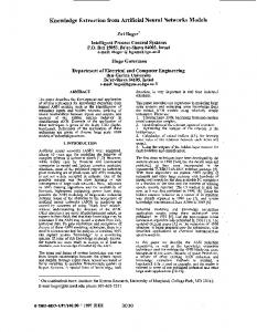
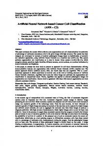
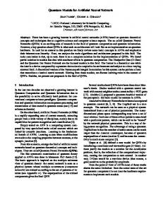
Sentences given an abstract tonal representation are converted to F 0 contours by means of phonetic implementation rules. These rules determine the F 0 values of tones and their temporal alignment with the syllables. The rules are calculated from left to right and they apply locally – any global trends (e.g., declination and rising intonation in questions) are caused by the sequence of tones and their interaction with each other. In a TTS implementation the tones, which are described in terms of their height and position, are connected to each other either by straight line interpolations or smoothed transitions in order to avoid discontinuities. The smoothing is accomplished by filtering the interpolated signal with e.g., a Hamming window [5]. Tone sequence models have been implemented for several languages including German, English, Chinese, Navajo and Japanese [53]. Unfortunately, no one has implemented a tone-sequence model for Finnish so far. 2.2.2 Fujisaki Model The Fujisaki model was developed for generating F 0 contours of Japanese words and sentences. The model is widely used in TTS systems and it has been applied to at least Japanese, German [49], English [17], Greek [20], Polish, Spanish [18] and French. The model is based on the assumption that any F 0 contour can be considered to consist of two kinds of elements: the slowly varying phrase component which consists of one or more slowly varying components, and a more quickly varying accent component (see Figure 2.3). These components are said to be
18
Chapter 2. An Overview of Existing Models for Prosody
related to the actions of the laryngeal muscles, specifically the cricothyroid muscle, which control the frequency of vibration of the vocal chords. Thus, the model has a physiological basis. The model is driven by a set of commands in the form of impulses (the phrase commands) and a set of stepwise functions (the accent commands) which are both fed to critically damped second-order linear filters and then superimposed to produce the final F 0 curve in the logarithmic domain which is then transformed to absolute pitch values. A good quantitative account of the model can be found in [19]. Figure 2.3 shows a Finnish sentence “menemmek¨o Lemille laivalla” (Will we go to Lemi by boat?) decomposed into its phrase and accent components. The figure depicts the signal waveform (on the top) followed by the actual pitch values (depicted by plus signs), the phonetic transcription (in Worldbet alphabet [22]) and the phrase and accent commands. The fitted F 0 curve from the model is drawn underneath the actual pitch values (the continuous line depicts the final contour and the dotted line the phrase component alone). 2.2.3 Tilt Intonation Model Taylor’s Tilt model [57] is based on the rise/fall/connection model that he introduced in [56]. Tilt is a bi-directional model that gives an abstraction for the F 0 contour directly from the data. The abstractions can then be used to produce a close copy of the original contour. In Tilt, each intonation event, be it an accent, a boundary, silence or a connection between events, is described by a set of continuous parameters. As an event-based model it is phonological in nature. The continuous nature of the parameters, however, give it a phonetic dimension that renders it very useful for prosody control in speech synthesis. The events are described by following parameters (see Figure 2.4): starting F 0 , amplitude (the distance between starting F 0 and the peak F 0 (amplitude is further divided to rise- and fall-amplitudes), duration (of the event in seconds), peak position (distance from the start of the first vowel of the
2.2. Intonation Models
19
J:innishdatawavs87
Fo [Hz] 240 180 120 60
Ap 1.0 0.2 Aa 0.6 0.2 0.0
# me n em:e k 7 l e m i l: e l
0.5
1.0
a
i v a l: a #
1.5
2.0
Fig. 2.3: An example sentence analyzed the Fujisaki model.
event and the peak of the F 0 event and the tilt, which is the result of dividing the difference of the rise and fall amplitudes by the sum of the rise and fall amplitudes [57]:
20
Chapter 2. An Overview of Existing Models for Prosody peak position rise amplitude fall amplitute
start F0
start of vowel
end of event
start of event
Fig. 2.4: The tilt model and its parameters. The final shape of the contour in this figure implies a tilt-value of approximately 0.25.
tilt =
| Arise | − | Af all | | Arise | + | Af all |
(2.3)
The tilt parameter gives the actual shape of the event with a range from -1 to 1. -1 is a pure fall, 0 is a symmetric peak and 1 is a pure rise. The shape in Figure 2.4 has a value of approximately 0.25. The importance of the Tilt model is in its ability to capture both phonetic and phonological aspects of intonation and its applicability to automatic speech recognition. This is due to its design goals which state that the model should have an automatic mechanism for generating F0 contours from the linguistic representation and that it should be possible to derive the linguistic representation automatically from the utterance’s acoustics [57].
2.3 Prosody Modeling for Finnish The most conspicuous aspect of any Finnish text-to-speech system is usually the lack of an intonation model.3 Segmental durations, however, are often quite well modeled; at least, the quantity degrees are well preserved and the 3
Some synthesis systems have a linearly descending pitch, which attempts to model the declination in F 0 . Others even give users the option of adding random fluctuations to pitch! And this is not to model the perturbation in the form of jitter found in real speech.
2.3. Prosody Modeling for Finnish
21
speech rhythm is acceptable. Most of the Finnish text-to-speech systems are proprietary and lack any documentation pertaining to the algorithms used for the models.
a depicts the Fig. 2.5: Matti Karjalainen’s intonation model for Finnish. b depicts the word-level component and c is sentence-level component, the superimposed signal used for F 0 control.
Arguably, the most sophisticated intonation and segmental duration models can be found in the Finnish version of the Infovox speech synthesis system. Nevertheless, even they are primitive compared to modern standards. The Infovox system is rule-based [11] and the intonation is carried out with less than 50 rules and a lexicon of less than 500 word-forms to separate function
22
Chapter 2. An Overview of Existing Models for Prosody
words from content words [61]. The segmental duration model is an implementation of Klatt-type rules. Matti Karjalainen and Toomas Altosaar [35] have used neural networks for duration modeling.4 Aaltonen [1] worked on a fairly sophisticated, syntactically driven intonation model in the 1970’s. Unfortunately, Aaltonen’s work was not continued. Matti Karjalainen also implemented an interesting superpositional model, which is presented in his doctoral thesis [34]. Figure 2.5 show the components of the model. The input to Karjalainen’s model was limited to syllabic segmentation and certain quantitative analysis of the input phoneme strings. The lack of prosody models does not imply that Finnish prosody itself lies in uncharted territory – on the contrary. It is only an implication of the fact that Finnish speakers as synthesis developers have usually been loyal to their intuition and misconception that there is no intonation in Finnish or that intonation is very simple and has direct correspondence to the written forms of the sentences. The misconception is most likely due to the fact the intonation is not in distinctive use in Finnish.
4
The segmental duration research described in this thesis is a continuation of that work.
Chapter 3 CHARACTERISTICS OF FINNISH PROSODY AND THE CORRESPONDING DOMAINS OF MODELING Finnish is among the languages that use morphology and morpho-syntax to convey certain types of information that in other languages are expressed by suprasegmental means. For instance, questions in more formal types of speech can be fully signalled by structural means – no specific intonation pattern is necessary. This ability is partly due to the free word-order in Finnish, which in turn, is a consequence of the rich morphology. The emphasis on linguistic structure has a bearing on the phonetic aspects of utterances – the structure, brought forth by rich morphology, has to be identifiable from the utterance, not vice versa. That is, prosody in Finnish may be more tightly coupled to the linguistic structure of the language than, say, in English. Finnish prosody is characterized by two conspicuous phenomena: the fixed place of word stress (always on the first syllable of the word) and the quantity system which strongly influences the segmental durations (and to a lesser degree the other parameters as well). The segmental degree of length (i.e., quantity1 ) encompasses all sounds of Finnish, thus in effect, doubling the phoneme inventory of 17 consonants and eight vowels to 34 consonants and 16 vowels.2 Statistically, quantity represents a high frequency phoneme within 1 2
For more information on Finnish quantity, see [45] and [76].
Not all sounds in Finnish take part equally in the quantity dichotomy; long /h/, /v/, /j/ and /d/ are marginal and long /j/ is very rare, occurring only in certain dialects and as a phonetic variant in words like [lyij:y] (lead). Long /b/, /g/ and /d/ occur only in loan words.
24
Chapter 3. Finnish Prosody and Domains of Modeling
the phonological system: there are 4074 long phonemes in our database of 692 sentences whereas the same data has 4608 /i/ and 4388 /a/ phonemes. The next most frequent phoneme is /n/ with 3515 tokens. A more detailed account of the data can be found in Appendix A. The two quantity degrees have an average duration ratio of roughly two to one.3 This ratio of lends credibility to the claim shared by most linguists and phoneticians who are familiar with Finnish that in fact the long phones stand for a sequence of two identical phonemes. Nevertheless, the distribution of durations is highly complex – this is best explained by an example; even though the first [a] in Figure 3.1 is more than twice as long as the second one, they are both perceived as short by Finnish listeners, furthermore the first [k] (whose quantity degree is long and is therefore perceived as long) is approximately equal in duration with the second one, whose quantity is short (it should be noted that the second [k] is word-initial; nevertheless, it causes no perception of an inserted pause). The lengthening of the short sounds is, of course, due to the fact that they reside in an accented syllable. A more detailed account of the distribution of durations and the effect of accentuation on durations in our data can be found in Appendix A. Since this research was concerned only with non-emphatic, declarative speech, no description of other kinds of utterances is given here. For a good overview of other types of utterances and of Finnish prosody in general, see [28]. The rhythmic structure of Finnish is straightforward with a strong syllable followed by zero, one or two weak syllables constituting a foot. A word is usually started by a new foot; see Figure 3.2 for a simple example and Section 3.1 for more detail. This is, of course, a simplification and does not 3
Ilkka Marjomaa [47] has found the average ratio between the durations of short and long phones to vary from 1:2.1 to 1:2.4 depending on speech rate (smaller ratio for faster speech). In our database of 692 sentences from one speaker the durations for long and short phones are 126.9 ms and 69.2 ms, respectively – this yields a ratio of 1:1.83. This is less than Marjomaa’s results and is probably due to the fact that Marjomaa had a fixed place for the opposition within an utterance whereas our results show the average over all occurrences of long phones in the data.
25
tarkka kirurgi varoo näköään tarkka t
A
r
kirurgi k:
A
k
i
0
r
u
varoo r
g
i
v
A 1.1
Time (s)
Fig. 3.1: Wave-form and transcription for the first two words in the sentence: “Tarkka kirurgi varoo n¨ ak¨ oa¨a¨n” (A meticulous surgeon is careful about his eye-sight). The durations for the first two [ ]-phones are 122 ms and 52 ms, respectively – similarly for [k] the durations are 122 ms and 118 ms.
include cases where the words have a more complex syllabic structure or when an utterance is started with a non-accented (or non-stressed) function word (the so called silent ictus), which usually does not occupy the beginning of a foot. Nevertheless, this simplification reflects the very basis of the rhythmic structure of Finnish. Another conspicuous aspect of Finnish prosody is that the linguistic function of fundamental frequency is much weaker than in most European languages – that is, intonation is not used for linguistic distinctions the way that is common among so called intonation-languages. This increases the relative importance of other prosodic parameters in carrying out the required linguistic distinctions. Segmental durations are especially important as they are the
26
Chapter 3. Finnish Prosody and Domains of Modeling Fs
Fw
Fs
Fw
σs σw
σs σw
σs σw
σs σw
jy . väs . ky . län . a . se . mal . la
Fig. 3.2: The stress structure for a phrase “Jyv¨ askyl¨ an asemalla” (At the Jyv¨ askyl¨ a station). Note that the long /l/ in the last word is – like all long consonants in Finnish – ambisyllabic.
most important factor responsible for the perception of phonemic length (for the relationship between F 0 and duration, see [73] and [4]). Loudness, on the other hand, has a trading relation with duration in the perception of prominence [60], which inevitably increases its significance. The following sections correspond to the domains (or levels) that were modeled throughout the investigation. With the exception of segmental durations, all three physical parameters were modeled on all levels independently (with the exception of loudness, which was not modeled on the sentence level).
3.1 Lexical Prosody Unlike the Indo-European languages, Finnish has a very central role for the word – as opposed to a phrase – as a grammatical and phonetic unit. This is due to the very rich morphology of the language. Most words in running text or speech are thus collections of both function- and content-related information and the distribution of actual function words is much more sparse than, for instance in English.4 For example, any noun in Finnish can have 4
Shattuck-Hufnagel and Veilleux [51] counted the percentage of function words in English text and found out that 48 % of the words are function words and the rest either, what
3.2. Segmental Prosody
27
more than 2000 different surface forms [38]. The grammatical information is always attached to the end of the stems as suffixes. Therefore, the last syllables of the word are usually functional/grammatical whereas the content resides in the beginnings (stems). This and the basic foot structure forces the lexical stress to the first syllable of the word. Most Finnish stems are bisyllabic and the most common stem-type is CVCV. The primary stress falls on the first syllable and the secondary stress on the third syllable which is always the strong syllable in the second foot of the word (see Figure 3.2 for an example). Even-numbered syllables are usually unstressed. This gives Finnish its characteristic rhythm. The fixed stress naturally serves as a place for accentuation – although the F 0 peaks do not always fall on the stressed syllable; see for instance [29]. Nevertheless, there is no dispute as to the perception of stress and accent on the first syllable of the word.
3.2 Segmental Prosody Finnish is among the languages where pitch-related microprosodic variation has been well attested; see for instance Aulanko [4]. Although the microprosodic characteristics work on the segmental level, they can be seen as the lowest level of a multi-layered system producing the final realization of the suprasegmentals in speech. The microprosodic variation is not generally considered to be a part of the linguistic or the prosodic pattern of the utterance, but rather to be something that is conditioned segmentally either by the identity of the segments themselves or by their immediate segmental context. That is, this variation reflects the specific articulatory movements that produce the sounds themselves. For instance, the fundamental frequency difference between open and close vowels and the effect of immediate consonant context on the fundamental frequency of a vowel seem to be universal they call intermediate words (adverbs, some prepositions, exclamations, post-determiners, quantifiers and qualifiers) (5 %) or content words (47 %). The percentage of function words in our database (692 sentences) is only 23.6.
28
Chapter 3. Finnish Prosody and Domains of Modeling
[75], [4], [74]. Similar variation can be observed with regard to loudness. The best-known phenomenon is the difference between the inherent loudness levels of, e.g., open vs. close vowels and sonorant vs. obstruent consonants [44]. If, however, one considers the final shape of the F 0 or loudness trajectory within a given segment to be a part of the aforementioned multi-layered prosodic system, the prediction of that shape will be dependent on information pertaining to all of those layers or levels. That is to say that microprosodic variation can hardly be abstracted away from the rest of prosody in a straightforward manner. Nevertheless, microprosodic variation is often left out of prosody models in text-to-speech systems. Some systems leave the microprosodic information in the concatenated units themselves and no further processing is done. Considering the amount of variation found in speech, this may not be the best approach unless one is willing to accept the necessary repercussions as to the size of the database or the quality of the output speech. Furthermore, great care has to be taken when the local events are superimposed on the global contour. The developers of text-to-speech systems usually regard microprosody as a set of a few well-known phenomena (the aforementioned intrinsic pitch and the effect of the immediate consonant context on the F 0 during a vowel or a voiced sonorant). This view is, perhaps, a little too simplistic and does not deal with the possibility that correctly modeled microprosody may well enhance the segmental intelligibility and naturalness of a system. The only microprosodic aspect of segmental durations would be the relative durations of the different parts of sounds that comprise more than one acoustically different chunk, such as stops and affricates. Nevertheless, no such phenomena have been investigated so far.5
5
Naturally, the final segmental durations are a product of an interplay between segmentally conditioned factors (e.g., inherent durations). Therefore, it can be said that in fact, certain microprosodic aspects of segmental durations were modeled by the addition of segmental and contextual information to the models’ input.
3.3. Sentence Level Prosody
29
3.3 Sentence Level Prosody Naturally, the word-level stress pattern of an utterance forms the basis for its accentuation pattern. The accentuation itself is carried out by the means of segmental durations (durations are longer in accentuated syllables (see Appendix A for more detail)), fundamental frequency and loudness (both have conspicuous peaks during accentuated syllables). 100
Hz 50
0 2
2.1
2.2
2.3
2.1
2.2
2.3
2.4
50
phon 25
2
2.4
0
2
2.1
2.2
2.3
2.4
time
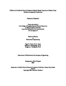
Fig. 3.3: The word “sikaa” in the sentence “tupakointi on siis t¨ aytt¨ a sikaa ja tupakoitsijat tulisi ampua l¨ ahimm¨ ass¨ a aamunkoitossa” (‘smoking, then, is pure swinery and smokers should be shot in the closest dawn’). The laryngealization visible in both the time waveform and loudness contour is used for signaling finality before a silent pause.
The basic declarative utterance in Finnish usually follows a gradually declining F 0 -curve with a corresponding loudness curve (although the loudness does not always undergo declination). This pattern is common for both
30
Chapter 3. Finnish Prosody and Domains of Modeling
statements and questions, which nevertheless, usually start with a higher F 0 than statements, but otherwise follow a similar declination pattern. Certain types of questions may, however, follow a different default pattern [26]. Finality is usually signaled with creaky (pressed) voice or an aperiodic (sometimes diplophonic) voice during the last (unstressed) syllables of the utterance. Continuation, on the other hand, is signaled by a higher level of F 0 before the boundary or some kind of laryngealization if there is a measurable pause within the utterance.6 Figures 3.3 and 3.4 show the two types of laryngealizations. The examples are from the sentence “tupakointi on siis t¨aytt¨a sikaa ja tupakoitsijat tulisi ampua l¨ahimm¨ass¨a aamunkoitossa” (‘smoking, then, is pure swinery and smokers should be shot in the closest dawn’).7 The first figure depicts the word “sikaa” which occurs before a silent pause and is therefore signaled by a laryngealization and a falling F 0 . Nevertheless, the change in F 0 is minimal (during the long [�� ] compared to the laryngeal effect that can easily be seen on the time waveform and loudness curve. The utterance-final word in the same utterance, on the other hand, ends with a creaky voice and a premature loss of voicing; see word “aamunkoitossa” in Figure 3.4.
6
This regular use of laryngeal gestures that are extremely difficult to detect in the F 0 contour of an utterance is one reason why it is very difficult to apply existing intonation models in Finnish. 7
This sentence is taken from the database of 692 sentences described in Chapter 4.
3.3. Sentence Level Prosody
31
75 50
Hz
25 0 5
5.25
5.5
5.75
50
phon 25
5
5.25
5
5.25
5.5
5.75
5.5
5.75
0
time
Fig. 3.4: The word “aamunkoitossa” in sentence “tupakointi on siis t¨ aytt¨ a sikaa ja tupakoitsijat tulisi ampua l¨ ahimm¨ ass¨ a aamunkoitossa” (‘smoking, then, pure swinery and smokers should be shot in the closest dawn’). The diplophonic voice, which can be seen in all displays is used to signal utterance finality.
32
Chapter 3. Finnish Prosody and Domains of Modeling
Chapter 4 DATA The research presented in this thesis has co-evolved with the Finnish Speech Database [3] in the sense that the scope of the study correlates with the inclusion of speech data in the database. On the other hand, the type of speech that has been included has largely been determined by the requirements of our research. Since the database initially consisted of isolated words, it was inevitable that lexical prosody was studied before moving into modeling whole utterances. The following sections give a short account of the different sets of data that were used for the research ranging from lexical prosody and microprosody on both lexical and sentence level to sentence level prosody with morphologically and morpho-syntactically tagged data. The current state of the database is shown in Table 4.1. Throughout the tests the material under study was divided into training and evaluation sets with the ratio of 2 to 1, respectively. This division was always based on random selection of data.
34
Chapter 4. Data
Description phonetically balanced isolated words phonetically balanced isolated sentences syntactically diverse sentences diverse sentences
Items/speaker Speakers
Labeling
2000
2 male
manual
117
2 male/female manual
276 1126
5 male 1 male
semi-autom. manual
Tab. 4.1: The contents of the Finnish Speech Database used for the studies (as of August 2000). The diverse sentences were further divided into questions (ca. 300 sentences), exclamations (ca. 100 sentences) and basic declarative sentences (ca. 700 sentences). A recording of these sentences by a female speaker is also in preparation.
4.1 Segmental and Lexical Level Experiments The segmental and lexical level experiments were run on several subsets of the database. These subsets were chosen according to the problem at hand – for segmental prosody studies at the word level, both isolated words and sentence material were used. The sentence material consisted of 117 sentences spoken by two male and two female speakers. The isolated words consisted of 889 phonetically balanced words with a wide coverage of different diphones and triphones spoken by two male speakers. Some tests were run on a 276 sentence, syntactically diverse (balanced) material spoken by five male speakers (this material was not, however, labeled by trained phoneticians and was not reliable for anything but very coarse pitch estimation). The material was prepared for a study on Finnish intonation [40]. Since loudness was only studied with the isolated word material, the varying signal amplitudes had to be normalized. A normalization scheme to keep the inputs for the loudness networks as constant as possible was devised. The scheme is described in [63]. The loudness curves for the study
4.1. Segmental and Lexical Level Experiments
35
Duration Distribution for Sentences (in seconds) 50 ’sentence-dur-dist.asc’ 45 40 35 30 25 20 15 10 5 0 1
2
3
4
5
6
7
8
9
10
11
Fig. 4.1: The distribution of sentence durations in the 692 sentence set of declarative sentences. The horizontal axis represents the duration of the sentences in seconds.
were calculated with the QuickSig signal processing system1 from auditory spectra. Two auto-correlation based pitch-detection systems were used for attaining the F 0 -curves for the material.2
1
The QS-system serves as an application development environment for the Finnish Speech Database [36] 2
One method was implemented in the QuickSig -system and some curves were calculated with the Praat program [9].
36
Chapter 4. Data
4.2 Sentence Level Intonation and Morphological Experiments For the sentence level experiments a database of 692 declarative sentences selected from a corpus of a Finnish periodical (Suomen Kuvalehti, 1987) was used. The sentences were selected randomly from a set of 60 000 sentences where the occurrence of foreign words had been minimized. Moreover, the lengths of the sentences (as phonemes) were kept between certain limits to keep their consequent durations within natural bounds with respect to speech production. The sentences were kept between 50 and 150 graphemes. The distribution of consequent sentence durations is shown in Figure 4.1. Figure 4.2 shows a typical isolated sentence in the database. The figure also depicts the typical creaky voice at the end of the utterance. This phenomenon is extremely common in this type of speech in Finnish (in our data more than 90 % of the sentences end with a creak). For this reason the experiments described in Section 6 which included sentence level pitch were run on everything but the last words in the data. The creaky voice and the premature cessation of phonation at the end of the utterances seem to be systematically distributed and merit a model of their own.3 The sentences were aligned with phonetic transcriptions with the aid of a Hidden-Markov-model based system (HTK by Entropic) and further manually corrected by a trained phonetician. The orthographic forms of the sentences were then analyzed morphologically by a two-level morphological tool (FINTWOL by Lingsoft Ltd.) and the analyses were further disambiguated by hand and attached to the word level transcriptions in the database. According to other researchers in the field, the study of prosody with a set of isolated sentences is bound to be doubtful as the “speaker has no emotional involvement in their content and no hearer for whom the message is intended, other than a microphone and any future listeners of the recording” [10]. However, V¨alimaa-Blum [68] argues that intonation in Finnish has 3
Since these phenomena are based on voice quality, they are impossible to model by the basic control parameters (F 0 , timing and intensity).
4.2. Sentence Level Intonation and Morphological Experiments
37
6 kHz
frequency 0 Hz 150 Hz F0 50 Hz
intensity
81 dB
37 dB 0.4404 0 –0.6982 2.513
0 Time (s)
Fig. 4.2: A typical sentence in the sentence level test set: “sellainen malli tuntuu vieh¨ att¨ av¨ alt¨ a” (Such a model feels charming). The typical creaky voice at the end of the utterance can be seen (the smaller box within the waveform display and the spectrogram). Note that although there is basically no detectable fundamental frequency during the creaky period, the intensity level remains fairly high. Note also that a typical pitch detection algorithm is unable to detect the F 0 at the end of the utterance; only two values are detected and even those are doubtful.
38
Chapter 4. Data
default forms that are directly related to the utterances syntactic form, its semantics and function, which is determined by its context. Therefore, it can be argued that the database of isolated sentences can be used for fruitful research on prosody. This is based on the grounds that the sentences are decontextualized and that the function of the sentences is neutralized or normalized (the function is simply to produce the decontextualized utterances as neutrally as possible). If there actually is a default form of intonation for each of the sentences, this may well be the only way to learn what that form is. Any deviation from the default will then be the result seen in longer stretches of speech or discourse that provide a stronger semantic and functional context for its parts. The deviations themselves are difficult to measure unless the default form is known beforehand.
Chapter 5 METHODS This chapter describes the neural network methodology used in our research. First, a short introduction to multi-layer-perceptrons is given followed by a description of their application to Finnish prosody.
5.1 A Short Introduction to Artificial Neural Networks Artificial neural networks are widely used in speech research today. Their uses range from acoustic pre-classification for automatic speech recognition [32] to full-scale neural net based synthesis systems ([33] and [37]). But what is an artificial neural network and why is it good for modeling prosody? Basically a “neural network is an interconnected assembly of simple processing elements, units or nodes, whose functionality is loosely based on the animal neuron. The processing ability of the network is stored in the interunit connection strengths, or weights, obtained by a process of adaptation, or learning, from a set of training patterns” [21]. A plethora of different types of artificial neural networks have been devised with the multi-layer perceptron (MLP) – especially when trained with the back-propagation algorithm – being perhaps the most widely used. An MLP consists of at least two layers of neurons; the hidden and output layers with a separate layer of nodes for the input. There is a certain amount of confusion as to the number of layers in the literature – some authors include the input layer in their description whereas other do not. Therefore, one encounters the terms two and three layer networks as describing similar architectures.
40
Chapter 5. Methods
...
Σ
... outputs to other nodes
inputs from other nodes
Fig. 5.1: An artificial neuron as found in most multi-layer perceptrons.
5.1.1 Artificial Neuron Figure 5.1 shows graphically the structure of an artificial neuron (or a node in neural network parlance). The following description describes both the input to the node and its activation in more formal terms. The input to a node or a neuron can be defined by the following equation: neti =
X
wij aj
(5.1)
j
This states that the net input is the sum of all inputs where each input is a product of node j ’s activation aj and the weight from j to i (wij ). The node’s response to the net input is determined by its response or activation
5.1. A Short Introduction to Artificial Neural Networks
41
Output (Activation)
1
0.5
0
−6
−4
−2
0 Input
2
4
6
Fig. 5.2: The logistic (sigmoid) function.
function. This function can be anything from a simple linear response to a so called logistic function: g(neti ) =
1 1 + exp(−neti )
(5.2)
Equation 5.2 defines a basic sigmoid function which is graphed in Figure 5.2. The sigmoid activation function makes the node act as a Threshold Logic Unit for both small and large inputs (i.e., it outputs either a 0 or a 1) but has a gradual and more sensitive response for inputs in the middle of its range.1 In these cases the nodes are capable of categorization even along dimensions that are continuous in nature [14]. This mixture of linear and nonlinear responses is what lies behind the behavior of these nodes and makes them so useful when grouped properly. Note that with the absence of input (i.e., when the input = 0.0) the nodes’ response is 0.5. It is often desirable to have a default activation other than 0.5 and a bias is used. The bias takes the form of an additional input (from a separate node) that is constant for a given node (although different nodes may have different biases). 1
This response is, in fact, linear and a network with sigmoidal activation functions contains a linear network as a special case [6].
42
Chapter 5. Methods
5.1.2 Network Architecture According to the description above, the network’s knowledge resides within the weights between its nodes as well as in the form of the network’s architecture – to be efficient, the architecture has to match the problem it is designed to solve. A network with an unfavorable number of units on any of its layers can be expected to be incompetent and inaccurate when compared to a network with the correct number of nodes. The determination of the correct architecture is, however, a trial-and-error process which reflects the theoretical views of the modelers.2 5.1.3 Learning in Neural Networks Since the knowledge within a network is represented by the weights between its nodes, a means to adjust those weights from their initial (usually random) values to something that best represents the solution to the problem at hand is needed. In other words, the network needs to learn and one needs a way to teach it. The most widely used training algorithm for multi-layer perceptrons is the so called error back-propagation or EBP. The aim of the algorithm is to adjust the weights from the output units to the hidden layer(s) and onwards from the units in the hidden layer to the input units in a manner which minimizes the discrepancy between the network’s output and its target, the desired output. In back-propagation this is done by propagating the error 2
It has actually been said that all of the modeling that a neural net is capable of can be expressed in standard, classical statistical means and the success of the neural net methodology reflects the cleverness of different input representations that modelers have designed. When our research is considered in this light, the verdict is not necessarily a bad one: this kind of methodology suits especially well the determination of the important factors in the symbolic domain that influence the physical aspects of prosody. There are two points that defend our choice of methodology: the networks’ ability to model the underlying interactions in the data which does away with some of the problems brought about by the nature of our data and the ability to use similar models for all of the physical parameters (F 0 , segmental durations and loudness).
5.1. A Short Introduction to Artificial Neural Networks
43
(i.e., the network’s output for a given training vector (t − o) subtracted from the target, or (ti − oi ) if there is more than one output node)) back to the network in such a way that the weights are gradually adjusted to optimal values. This process is in no way deterministic and the networks do not always converge on the same solution. Elman and his co-authors give a simple formal account of the back-propagation algorithm in [14]. The existence of target values implies that multi-layer perceptrons gain their knowledge in a supervised manner. This is in stark contrast with the real world where most learning is done without supervision. This kind of learning is captured in networks that are capable of learning without supervision – Teuvo Kohonen’s Self Organizing Maps (SOM), [42] being a prime example. 5.1.4 Pre- and Post-processing Since the input to the network can only be numerical and text is graphical in nature, a pre-processing phase is needed. That is, the textual representation of speech has to be transformed into a numerical representation. The fact that the networks’ mapping serves a general purpose implies that less emphasis is needed as to the care of optimizing the inputs than is the case with simple linear techniques, e.g., multiple linear regression (see [65] for an example). This is not to say that one can go about pre-processing carelessly. In the case where the (input) data has to be transformed into another representation (as opposed to transformations within representations), the network’s performance is directly dependent on the amount of prior knowledge incorporated in the input. In relation to prosody, the prior knowledge dictates what information that is known to have an influence on the prosodic parameters should be included in the input. For instance, the phonetic context is known to affect segmental durations and should, therefore, not be left out of the model. Prior knowledge should also be used to determine how to post–process the network output – the output coding should reflect the way the parameters are distributed. For instance, it is well known that segmental durations
44
Chapter 5. Methods
input data preprocessing
neural network
postprocessing
output data
Fig. 5.3: Schematic illustration of the use of pre- and post-processing of data for neural network mapping (after [6]).
follow a logarithmic distribution and it is, therefore, more practical and advantageous to use the logarithm of the duration as a target value. Moreover, the logarithm can be further coded so that the mean of the durations is located in the middle of the sigmoid response function. Figure 5.3 shows the process of pre- and post-processing in conjunction with a neural net mapping (after [6]). In our case, the pre-processing stage refers to the transformation of text and linguistic structures to numerical inputs (see Section 5.2.1 for more detail) while post-processing refers to the target and output coding of the physical parameter values to match an optimal output from the networks. In order to get a final output from a network, the coded values have to undergo the inverse of the original output coding. 5.1.5 Feature Selection In order to make the problem easier for the network to model, some information in the training data has to be ignored. That is, not all information inherent in the data is useful for training. For instance, defining phonetic contexts with phone identities rather than grouping them under broader classes increases information in the training data without giving the network any advantage. The process of reducing the dimensionality in the input is called feature extraction or feature selection. Given a linguistic input, feature selection can be based on prior linguistic knowledge. In this case, the features are the well-known phonological and linguistic ones that can be calculated from the textual input. The reduction of dimensionality by grouping the features or by representing the units by higher-level features (e.g., using the feature nasal rather
5.2. Neural Network Methodology Used in this Research
input text
45
duration
− linguistic analysis − morphological analysis − syllabification −etc.
loudness
segmental F0
+
F0 contour
global F0
input coding
neural networks for all physical parameters and levels
output coding
Fig. 5.4: A global view of the model for prosody control proposed in this study.
than the phone identities [m],[n], and[ ]) works to our advantage in two ways: it reduces the scarcity of data by reducing the number of different feature vectors and it ensures that only the relevant information is given to the networks to learn from. Naturally, most of this linguistic knowledge is discrete. To avoid artificial ordering, certain care must be taken when coding it.
5.2 Neural Network Methodology Used in this Research Figure 5.4 shows the overall architecture of the model for prosody control described in this thesis. In our experiments the network’s task was to compute from one to three values (duration, average pitch, average loudness-level or any combination therein) for a known phoneme in a context defined by the phoneme sequence within a word or a sentence and additional information pertaining to the
46
Chapter 5. Methods
syllable, word or utterance in question.3 Since the sentence level experiments with morphological information required the most complex input representation which actually included all of the input used for the earlier experiments, it is sufficient to describe only the final composition of the input vectors here. It should be noted that this coding scheme differs in minor details from the one used for lexical and microprosody experiments. However, the differences are not significant and have no bearing on the final results. Each type of network (duration, loudness or pitch) was given an identical training vector. The composition of the training vector was varied systematically throughout the tests. In order to determine the optimal network size for a problem, the number of input and hidden nodes in the networks was varied. This was done by varying the length of the phone context window, choosing different factor combinations for the network input and varying the number of hidden nodes in a systematic manner. All results from the tests are described in Chapter 6. Since the network architectures and data representations for different tasks were kept as similar as possible throughout the tests, certain inferences could be made from the influence of the different factors on the parameters’ behavior.4 The basic network architecture used was based on a two-layer perceptron5 architecture with fully connected nodes throughout (see Figure 5.5). The activation function of the nodes in the hidden layer as well as the output node was a basic sigmoid. The networks were all trained with the standard back-propagation algorithm.
3
Only a few tests were run for concurrent parameter prediction for the reason that a set of specialized nets always performed better than a network trained to predict more than one parameter at a time. 4
This will hopefully make the system’s transition from the laboratory to the real world a little less painstaking. 5
Feed-forward network is practically synonymous with multi-layer perceptron. It should also be noted that some authors use the concept of layer to include the input nodes. Thus the networks employed in this study would consist of three layers.
5.2. Neural Network Methodology Used in this Research
Input layer
Hidden layer
47
Output layer
Fig. 5.5: The basic neural network architecture used for all experiments. The layers are fully connected. The activation function in both the hidden and output layers is a sigmoid. The output of the network is either a coded loudness value, a coded fundamental frequency value or a coded segmental duration.
Since this study was concerned with the relative importance of different linguistically motivated factors in the network input, the optimal performance of the networks was not always the primary goal. It may even be argued that the basic MLP methodology is not well suited to the problems at hand – intonation and segmental duration modeling on the level of utterances. For instance, recursive networks have enjoyed better success in modeling intonation [59]. However, Campbell [10] has successfully used a similar methodology for segmental duration modeling. It must be emphasized that the models described here do not attempt to predict F 0 or loudness curves per se, but instantaneous values within an utterance. The models simply map values between a phonetically and linguistically motivated input vector for a certain unit in a sequence and a
48
Chapter 5. Methods
corresponding physical parameter. Any curve or trajectory is just a sideeffect of predicting values for a sequence of vectors that earn their cohesion from being calculated from the same utterance and being reconstructed into a similar sequential order. This is important when one looks at the problem from the point of view of selecting the right kind of neural network architecture for a given task. Viewed in this light, it should be clear that no time series estimation or forecasting is being done with the models presented here and therefore the networks do not need to have information about their prior behavior. That is, a simple multi-layer perceptron trained with backpropagation is sufficient for the purpose. No explicit prosodic information was used. Therefore, the networks’ task was to associate the given prosodic value (pitch in semi-tone, logarithmic duration) with the symbolic information in the linguistic and spatial description of the sentence. The final input to the network consisted of coded values for the current phone or syllable and the current word. Also, a window of three units on either side of it was similarly coded and added to the input vector. Thus the duration network’s input consisted of word-related and phone-related data covering a certain span of the input text as well as data concerning the place and size of the current units in the sentence (see Figure 5.7 for more detail). The neural networks were trained speaker-dependently, i.e., one or more models were generated for each speaker. The individual coding schemes are described in the following papers: lexical experiments [62]; microprosody for pitch and loudness (isolated words) [65]; microprosody on the sentence level [64], [63] and [66] and sentence level prosody augmented with morphological and morpho-syntactic information [67]. 5.2.1 Input Coding Input Data Representation – Words Tables 5.1 and 5.2 show the factors that were given as input to the networks. All factors were translated to a numerical representation so that the values
5.2. Neural Network Methodology Used in this Research
49
Region of input vector dedicated to phonetic context
Current phoneme: − identity − broad class − quantity degree Nearest neighbor: − broad class − quantity degree Other neighbors: − consonant vs vowel − quantity degree
Fig. 5.6: The representation of phonetic context in the neural network input.
varied between 0.0 and 1.0. Those factors that had more than three levels (e.g., case with 15 levels) were distributed to two nodes. This is akin to the 1-of-C coding scheme described in [6]. As can be seen in Table 5.1, most of the morphological factors concern words of a certain part-of-speech only; e.g., comparation is inherently connected to adjectives. Verbs on the other hand have more morphological features and more factors attributed to them than other words. Whenever a factor was unrelated to the word being coded, a small, non-zero value was added to the input vector. Thus, it made no sense to test each morphological factor’s influence against the whole set of words and the morphological factors were tested as a whole against other factors (see Section 6.3 for more detail). Input Data Representation – Phonemes The information relating to phones and phonemes for coding the phonetic context consisted of three different levels of description depending on the proximity of the current (predicted) phone to the rest of the phones included
50
Chapter 5. Methods
Morphological factors Values Number of nodes Comparation Case Number Mood Tense Voice Person Negative Infinitive/participle Suffix
3 14 2 4 2 2 7 2 6 2
1 2 1 2 1 1 2 1 2 1
Tab. 5.1: The morphological factors concerning words and the number of necessary values that were coded as input to the networks.
Coded factors Function word Punctuation Compound word Part-of-speech Place in syllable Place in word Place in sentence Length in phones Length in syllables Length in words
Number of values
Number of nodes
2 2 2 15 continuous continuous continuous continuous continuous continuous
1 1 1 2 1 1 1 1 1 1
Tab. 5.2: Other types of information pertaining the phone, word and sentence in question and the number of values needed.
in the input. That is, the phonetic context was described in a heterogeneous way.
5.2. Neural Network Methodology Used in this Research
51
The coding of the current phoneme included its identity and broad class broken down between two nodes and its length degree. The nearest neighbors to the current phoneme were coded according to their broad class (e.g., nasal) and their length. Any further phonemes were coded as either vowels or consonants and being either short or long. See Figure 5.6 for more detail. Input Data Representation – Size and Place
Fig. 5.7: The hierarchical coding of relative position and size of the current (estimated) phone or syllable. In this case the phone [v] is being estimated and its place is coded according to its position in the syllable [va] of length two (phones). The syllable’s position is coded in relation to the word [va . roo] with a length of two syllables. The word is further given a code according to its place in the sentence /tarkka kirurgi varoo n¨ ak¨ oa¨a¨n/ with a length of four words (“A meticulous surgeon is careful about his eyesight”). This yields six values for the networks’ input vector that concisely describe the relevant units’ places in the hierarchy as well as their lengths: 0.0 and 0.2773 for the phone; 0.0 and 0.2773 for the syllable; 0.6666 and 0.5546 for the word.
Finally, the relative position of the estimated phone within the word, syllable and sentence was added according to a scheme that takes into account the units’ sizes and position in a hierarchical representation of the utterance; see Figure 5.7 for more detail.
52
Chapter 5. Methods
5.2.2 Output Coding In all but the microprosodic experiments the network’s output consisted of a single value for each phone, or, in the case of sentence level F 0 experiments, a syllable. In the microprosody experiments three to nine values were generated for each (voiced) phone. In order to yield a single value for loudness and pitch, the original time functions were reduced to an average for each phone. The central third of the whole phone was chosen as the span to be averaged. Naturally, for segmental level, microprosodic networks, no averaging was needed and the networks were trained to predict from three to nine absolute pitch or normalized loudness values for each phone. This was done to capture the shape of the pitch or loudness contour during the predicted sound. It is a well known fact that segmental durations follow a normal distribution on a logarithmic scale (see Figure 5.8). Therefore, the network was output coded to yield the logarithm of duration which was further coded so that the values remained between 0.0 and 1.0. Similarly, the output of the pitch-network was the frequency value in Hertz converted to semitones which was further coded to a value between 0.0 and 1.0. The network error was simply the target value minus the output value, i.e., (t − o). The errors reported in Section 6 are all average absolute errors in percent: thus, an error of 5 % for pitch would be 5 Hz at 100 Hz. Thus, the target values for the networks were as follows: • Duration networks: log of duration (mapped linearly to values between 0.0 and 1.0) • Pitch networks: semitone (mapped linearly to values between 0.0 and 1.0) • Loudness networks: phon (mapped linearly to values between 0.0 and 1.0) In order to study the influence of morphological information on the networks’ performance to predict F 0 values, the syllable nucleus – instead of a
5.2. Neural Network Methodology Used in this Research
53
Raw and Logarithmic Distributions for Segmental Durations ’duration-distribution.asc’ ’duration-distribution-log.asc’
Fig. 5.8: The distribution of durations in the 692-sentence database: both raw durations in milliseconds (leftmost, skewed distribution) and logtransformed durations are plotted.
single phone – as the predicted unit, was chosen. Thus, the target value for the network was an averaged F 0 value for the center one third of the syllable nucleus. This is a very coarse way of calculating the pitch values for it ignores partially the shape of pitch accents as well as their exact placement in relation to the syllables. It also produces a fairly large margin of error concerning the values usually deemed important in relation to perception of pitch, that is, the peaks and valleys of the pitch contour as well as their placement in relation to the syllable nucleus.
54
Chapter 5. Methods
Chapter 6 RESULTS
This chapter summarizes the results from the various experiments which were conducted during the research. The results are presented in a conceptually motivated order that does not necessarily reflect the order in which the studies were conducted. The discussion of results from the lexical and microprosodic studies are basically duplicated from the publications (see the list of publications on page xxv) with a little more discussion added, whereas a more detailed discussion of the results from the sentence level studies is given. The overall results obtained in all of the experiments are very encouraging and point to possibility of using this methodology, as it is, for prosody control in a TTS system (see Chapter 7 for more details). Since the modeling task for isolated words – as opposed to isolated sentences – is less complex in nature, it is not surprising to find that the results are better as well. All in all, the results for segmental and word level prosody stay within the perceptual thresholds for speech, whereas the results for sentence level networks generally perform somewhere in the area around the thresholds as reported in the literature:
• Networks modeling word level loudness achieved an average error of 2.2 phon whereas segmental level networks error was 2.6 phon at best (1 phon is generally considered just noticeable for non-speech sounds), whereas the just noticeable difference (JND) for more speech-like sounds
56
Chapter 6. Results
varies from 1.0 to 4.0 dB1 [54]. • Networks modeling word level pitch achieved an average error of 3.5 % which corresponds to about 0.6 semitones and is well below the 1.5 to 2 semitone JND for speech [55]. • Networks modeling segmental duration on word level achieved an average error of approximately 12 %, which is well below the 20 % threshold for Finnish as reported in [35]. • Networks modeling segmental duration on sentence level achieved an average error of approximately 17 %. • Networks modeling pitch on sentence level achieved an average error of approximately 8 % (1.33 semitones), which is within the JND for pitch perception in running speech. Nevertheless, it must be emphasized that the errors reported here are averages and the networks sometimes make predictions that are well beyond the reported thresholds. This is especially the case with sentence level networks. Some analyses of the errors are discussed in Section 6.3.
6.1 Segmental Prosody As mentioned earlier, segmental or microprosodic variation was studied in relation to F 0 and loudness. Table 6.1 shows the performance of the segmental level networks on both pitch and loudness. The values in the table are average absolute errors in percent and do not depict the networks’ ability to predict the actual shapes for the contours during the predicted phone; this can be seen in Figure 6.1 which shows the performance of an F 0 network against actual data. It should be mentioned that these tests were run on 1
At the loudness and frequency ranges of speech the phon and dB scales are practically equal.
6.1. Segmental Prosody
57
isolated words which are, as a matter of fact, always accented. This simplifies the network’s task in the sense that it can predict the accentedness from the position of the current phone and its phonetic context.2 Accentedness, naturally, defines the basic shape of the given contour during the phone; e.g., the shape of the F 0 contour during accented vowels often contains a clear peak whereas unaccented vowels tend to have flat3 or concave shapes. Nevertheless, the F 0 shapes of accented phones (especially vowels) vary greatly depending on the segmental make-up and context of the current syllable. This can be seen in Figure 6.1 where the shapes of the two accented [ ] vowels are markedly different (lower left and middle right panes). The networks’ good ability to predict the shapes of the F 0 and loudness curves was, therefore, partly due to the fact that they did not need to predict whether a given phone was in an accented syllable or not; this information was directly related to the position of the current syllable in the word.
2
This is, naturally, due to the fact that lexical stress in Finnish always falls on the first syllable of the word. However, this does not mean that the consequent F 0 and loudness peaks occur during the lexically stressed syllable; see for instance the first word (“olennaisia”) in Figure 6.6. 3
That is, more or less linear shapes that are either rising, falling, or level.
58
Chapter 6. Results
normalized pitch (Hz)
[tuuli]
normalized pitch (Hz)
[ladata]
normalized pitch (Hz)
[gal:up]
[tase] relative time
[knal:i]
[tase] relative time
Fig. 6.1: Examples of F 0 networks’ results (circles) plotted against natural data (squares) (from [65]). The current or predicted phone is printed with bold-face letters.
Table 6.1 summarizes the results for a group of networks with a varying degree of specialization for two male speakers (two sets of identical words spoken by the speakers). It is fairly conspicuous that the results for Speaker 1 are generally better than for Speaker 2 – only in two out of sixteen cases are the results better for Speaker 2. This may be a consequence from a multitude
6.1. Segmental Prosody
59
of factors – however, Speaker 1 had (at the time of recording) much more experience in speaking in an anechoic environment, which lead to much less prosodic variation in the material. Speaker 2, on the other hand, tended to over-articulate the words leading to unnaturally long segmental durations at times as well as unnaturally large variation in loudness.4
Pitch (% error)
Loudness (error in phon)
Network trained for: Speaker 1 Speaker 2 Speaker 1 Voiced Vowel Sonorant Voiced Stop Unvoiced Fricative Unvoiced Stop [ ] [l] [s] [] �
1.66 1.39 1.76 1.40 1.18 -
2.07 2.01 1.88 2.18 1.74 -
2.61 1.76 3.05 4.59 3.66 2.55 3.18 1.37 2.48 2.33 3.28
Speaker 2 3.22 2.50 3.45 3.56 4.45 3.28 3.39 1.76 2.30 2.53 2.32
Tab. 6.1: Segmental level network estimation results (average absolute error in percent) for pitch and loudness — two male speakers. The pitch values are in Hertz (average percent error) and the loudness values are average phon. The values for [ ] are for the release phase only. The term “sonorant” refers to voiced, continuant consonants (from [63]). �
4
�
The 889-word material used for both segmental and word level prosody experiments was recorded in an anechoic environment without auxiliary auditory feedback for the speaker (e.g., headphones), which in the case of Speaker 2 lead to some compensatory raising of the voice and consequent (and somewhat unpredictable) prosodic variation.
60
Chapter 6. Results
6.2 Word Level Prosody The term word level, as used here, refers to the fact that these tests were run on isolated words. Naturally these words are bound to have a residue of prosodic variation from larger domains; mainly the utterance. The material was, however, recorded in a manner which minimized sentence or utterance level effects; the words were each spoken three times with a small pause between the tokens. Since the tokens were identical, the speakers were able to avoid an obvious list intonation. The possible prepausal lengthening effect was also minimal – by a rough estimate, over ninety percent of the time the middle token was used for final data and the rest of the tokens were discarded. This section describes the results from a series of three tests which were run to determine: • the level of specialization necessary for adequate prosody control, • the effect of the size of phonetic context on the network performance, and • the relative importance of different input factors to the networks. 6.2.1 Specialization It is often the case that the networks need to specialize on a subset of objects in order to minimize the overall error over all types of units in question. Specialization turned out to be critical with networks predicting segmental durations on the word level. For optimal performance, 16 networks – which were categorized according to natural phonetic or phonological classes – had to be trained. Figure 6.2 depicts the results of specializing a set of networks for lexical level segmental duration prediction. On the other hand, estimating either average pitch or loudness levels turned out to be more straightforward — dividing the task to cover only a subset of phones did not yield comparatively better results. The figure shows the error percentages for a set of duration networks that were trained for one speaker’s data of 889 words. The tree depicts the optimal distribution of networks for the task. The leaves of
6.2. Word Level Prosody
61
the tree comprise the optimal set of networks with an approximately 12 % average error.
Short Short Vowels Vowels 12.0% 12.0%
Short Short Phones Phones 18.1% 18.1% Vowels 13.8 %
Long Long Vowels Vowels 7.3% 7.3% Short Short Consonants Consonants 18.5 18.5 % %
All All Phones Phones 16.9% 16.9%
Stops 12.5 %
Consonants Consonants 19.5 19.5 % %
Long Long Phones Phones 7.7% 7.7%
Nasals Nasals 19.5 19.5 % %
Short Short 13.0 13.0 % % Long Long 5.0 5.0 % % Short Short 17.8 17.8 % % Long Long 8.5 8.5 % %
Fricatives Fricatives 14.0 14.0 % %
Short Short 14.2 14.2 % %
Semivowels Semivowels 21.1% 21.1%
Short Short 19.7% 19.7%
Long Long 10.4 10.4 % %
Long Long 10.6% 10.6%
Long Long Consonants Consonants 11.0 11.0 % %
Fig. 6.2: Error percentages for lexical level duration networks (from [64]).
There is a consistent difference in the networks’ performance in relation to the long vs. short categories of phones; e.g., the error for a network trained on long stops is only 5 % as opposed to 13 % for short stops. It is not immediately clear why it is so and further analysis of the training data is needed for an explanation. With respect to the number of occurrences, the short phones outnumber the long ones with a ratio of nine to one. This, however, does not
62
Chapter 6. Results
explain the difference in performance – neither does the overall variability in the absolute or raw durations. The standard deviations for the long and short durations are 0.067 s and 0.054 s, respectively. The log-transformed durations, on the other hand, reveal a different picture with the short durations having a relatively large standard deviation compared to the long durations (0.55 vs. 0.20, respectively). The relatively small variability of the durations of the long phones may be due to various reasons: the long/short distinction has to be maintained, without exceeding certain boundaries which may be rhythmically determined. Moreover, long consonants cannot occur in word-initial or word-final positions where their durations are bound to vary more due to residue from phrasal factors. The relatively good performance, then, is due to the fact that the networks were trained to predict durations in the logarithmic domain and the smaller variance in that domain make the networks’ task easier. 6.2.2 Effect of Context Size Figure 6.3 shows the effect of phonetic context on a duration network. The y-axis stands for prior context and the x-axis for context after the current phone as a number of phones. The context is measured as the number of phones on each side of the current one. The figure clearly indicates that increasing the contextual information has a beneficial effect on a network’s performance. One conspicuous fact is visible in Figure 6.3; after a context size of ±2, increasing the right context leads to no improvement in performance whereas increasing the left context has nearly the same effect as increasing both contexts at once. This finding is difficult to interpret due to small size of training data. Nevertheless, the results beg for an intuitive interpretation concerning speech production; it seems that the already produced segments have more influence on the duration of a given segment than the ones still in planning. This gives support to the claim that the duration of a word-final vowel in a CVCV word in Finnish is influenced by the length of the preceding vowel and not vice versa (see for instance [45] and [76]). A similar effect could be
6.2. Word Level Prosody 4
63 13
15
13
14
16
14 17
13
13
14
15 16
3
14 15
Left Context
17
14
16
14 2
15 18
17
15
15
16 16
19 1
20
20 0 0
18
19
19
17
15
16
16
16 17
17
15
17
17
18
17 18 1
2
3
4
Right Context
Fig. 6.3: Average absolute relative errors for a duration network trained to estimate vowel durations as a function of the input vector’s composition. The horizontal axis represents the right context and the vertical axis the left context as numbers of neighboring phones. Each pair is an average result of five separate neural networks trained for 500 training iterations of the training set. The minimum error (12.26 %) occurs at (-4,4) and the maximum error (20.14 %) at (0,0). From [64].
observed for F 0 but not for loudness.
64
Chapter 6. Results
6.2.3 Relative Importance of Different Input Factors A study to determine the effect of adding different factors to the network input was also carried out. This was done in order to measure the factor’s relevance and influence on the behavior of the physical parameters. These results are shown in Figure 6.4. The methodology to obtain these values was similar to the one described in Section 6.3. That is, the aggregate improvement of network performance when a certain factor (e.g., phoneme identity) was added to an otherwise similar network input was measured. Having six different factors to test lead to 26 − 1 = 63 different combinations of input to test.5 The improvement, then, was the averaged difference between the networks’ error before and after adding a factor. For n factors. each factor was added 2n /2 times to the input. The final results are averaged for five different test runs. All in all, 315 networks were trained and tested. Each network was trained for 500 cycles and the minimum evaluation error was used for the result. In summary, the results state the obvious: phoneme length is the most important factor in relation to segmental durations followed by phoneme identity, which points to the well known fact that phones have intrinsic durations. A more interesting result is that phoneme identity seems to have practically no effect on the pitch networks’ performance. This suggests that the intrinsic pitch, as described in [4] and [75], may not be realized in other than tightly controlled test conditions and material.
5
The omitted combination stands for the lack of any input; a network without input generates a random output and cannot be used as a measure against other factors.
6.3. Sentence Level Prosody
65 8
Duration
7
10 Average % improvement
F0 8
6
Loudness
5
6
4 3
4 2 2 1 0
Average improvement Hz (F0) Phon (Loudness)
12
0 PNUM
SNUM
PLEN
SPOS
PPOS
PID
Factor
Fig. 6.4: Averaged values for different factors’ effect on the network performance: pitch and loudness (right) and duration (left). The y-axis represents the average decrease in average percent error when a factor is added to the input vector. The results are for two speakers (MK and MV). The abbreviations are as follows: PNUM, number of phonemes in word; SNUM, number of syllables in word; PLEN, segmental length (long vs. short); SPOS, syllable position in word; PPOS, phoneme position in word, PID, phoneme identity. From [64].
6.3 Sentence Level Prosody On the sentence level 6 two different problems bearing on the modeling were of interest: on the one hand the relative importance of grammatical – mainly morphological – information had to be determined and, on the other hand, the prediction accuracy had to be determined. Results from adding morphological information to the network input are discussed in Section 6.3.1. Specialization, as discussed in the previous section, had no considerable effect on sentence level network performance. The context size was kept constant 6
The terms sentence and utterance are used interchangeably here.
66
Chapter 6. Results
at ±3 words and phones throughout the tests. As the modeling task becomes more complex with longer stretches of speech, the actual performance of a single network becomes more important. Therefore, a series of investigations on the network error was conducted and the results are discussed in section 6.3.2. 6.3.1 Influence of Morphology on Network Performance Morphology has traditionally played a minor role in prosody research and prosody control in TTS. Finnish is, however, a language in which morphology plays a very central role and a question naturally arises as to what degree does it influence prosody? A test to determine the influence of morphological information on the networks’ performance was conducted in a following manner:7 1. Three factors had to be tested: these were the part-of-speech and function-word status of the words as well as the morphological values of the words as a set. Three factors yielded eight combinations (i.e., 23 ).8 2. The effect of each factor was determined by averaging the differences in the performance of the different networks. Within the eight combinations, each factor was supplied four times and omitted four times (i.e., 23 /2). 3. Once all tests had been run (that is, all different networks representing different combinations), the differences in the performance level were calculated and averaged for each factor. The results from each combination were averaged over five different networks. 7
This test is basically the same which was used for assessing the relative importance of input factors for word level prediction (see Section 6.2 for more detail). 8
Unlike the word level networks, there was always some input in the form of spatial coding (see Section 5.2.1) to the network and it was not necessary to omit the “empty combination”.
6.3. Sentence Level Prosody
67
Table 6.2 shows the average reduction in error (%) when different kinds of information to the network input for both segmental duration and F 0 were added. The value for function word status is binary, whereas the other values are more gradual (see Section 5.2.1 for more detail). It can be seen from the results that when morphological information is added to the network input the performance of the networks increases. However, the significance of the drop in error is fairly difficult to assess in quantitative terms and perception tests should be conducted to determine the final significance of the results. The improvement is largest for segmental durations which seems to point to a higher level of interaction between segmental durations and morphology. The results from the F 0 networks, on the other hand, can be explained by the fact that including morphological information to the network input gives the network a better possibility to generate hypotheses about the implicit linguistic structures within the sentences. The networks may be said to implement some sort of a statistical grammar model akin to the so called n-gram models, which in turn helps the network in determining those prosodic boundaries that coincide with (or depend on) the syntactically determined boundaries. F0 Function word Part-of-speech Morphology
Average decrease in error (%) -0.15 -0.40 -0.71 Duration
Function word Part-of-speech Morphology
Average decrease in error (%) -0.61 -0.28 -1.16
Tab. 6.2: Results from adding morphological information, function word and partof-speech status to the network input (from [67]).
68
Chapter 6. Results
6.3.2 Modeling Accuracy Figures 6.5, 6.6 and 6.7 show three randomly selected sentences and their annotations on the sentence, word and phone levels from the evaluation set of a network trained to predict F 0 values on a syllabic basis. The grey lines depict the actual (interpolated) F 0 contour and the dotted line the network’s predictions for all but the last words in the utterances. The network was trained for 100 cycles and contained 30 hidden nodes. It should also be noted that the network was not trained to predict values for the syllables in the last words of the utterances (see Section 4.2 for more detail).
Frequency (Hz)
150
0 0
4.551 Time (s) intellektuelliksi joko synnytään tai julistaudutaan .
intellektuelliksi
i n t[ e l: e k
t[ u e
joko
l: i k s i j o k o s
synnytään
y
n: y t[
tai
@: n t[ A i j u l i s
julistaudutaan
t[ A u d u t[
A:
n
Fig. 6.5: The sentence “Intellektuelliksi joko synnyt¨ aa¨n tai julistaudutaan.” (One is either born as an intellectual or one announces to be such.). Note that the first predicted value (not produced by the network) is arbitrarily set at 100 Hz.
The figures show distinctly that the networks are capable of predicting accent placement very accurately. That is to say, the networks are capable of capturing the phonological aspects of intonation whereas the more phonetic aspects still lack precision. It is interesting, however, to notice that the networks are quite accurate in predicting values for unaccented syllables –
6.3. Sentence Level Prosody
69
Frequency (Hz)
150
0 5.828
0 Time (s) olennaisia toimintoja saa käsikirjoista etsiä kummallisuuksien seasta .
olennaisia
toimintoja
saa
käsikirjoista
etsiä
o l e n: A i s iA t[ o i m i n t[ o j A s A: k @ s i k i r j o i s t[A e t[ s i@ k
kummallisuuksien
seasta
u m: A l: i s u: k s i e n s e A
s t[
A
Fig. 6.6: The sentence “Olennaisia toimintoja saa k¨ asikirjoista etsi¨ a kummallisuuksien seasta.” (One has to look for essential functions in the manuals from the midst of peculiarities.).
especially in a relative sense within words . This seems to point to the fact that – at least with regard to speech production9 – the stretches between so called important parts (accented syllables) are not so uninteresting after all and do not merely happen [43]. The details in Figures 6.5, 6.6 and 6.7 are difficult to interpret. Nonetheless, there are certain things which are evident: function words (including copula) are always unaccented10 and verbs are either accented or not depending on their function – something that the network has to infer from the relative position and morphological analyses of the words. For instance,
9
’t Hart, Collier and Cohen have shown that the level of detail visible in Figures 6.5, 6.6 and 6.7 may not be necessary in relation to perception. Nevertheless, the fact that the networks are able to capture such detail makes it relevant with respect to speech production. 10
Accentuation is simply determined by an occurrance of a clear peak in the F 0 curve.
70
Chapter 6. Results
the passive verb “julistaudutaan” (is announced ) in Figure 6.5 is accented as opposed to the members in the verb chain “saa etsi¨a” (one (gets—is forced) to look for ) in Figure 6.6 which are unaccented. Another interesting detail is the division of the intonation curve into two prosodic phrases or units in Figure 6.7 between the words “nuorisolle” and “taiteilija”.
Frequency (Hz)
150
0 0
7.5 Time (s) taiteilija aaltosen tuomio on näyttänyt huonoa esimerkkiä nuorisolle , taiteilija aaltonen itse ei niinkään .
taiteilija
aaltosen
tuomio
on näyttänyt
huonoa
esimerkkiä
nuorisolle
t[A i t[ e i l i j A A: lt[os en t[ u om i o o nn@y t[:@nyt[ h u o n o A e s im e r k: i@n u o r i s o l: e
taiteilija
aaltonen
itse
ei
niinkään
t[A i t[ e il i j A A: l t[ one n i t[ s e e i n i: N k @: n
Fig. 6.7: The sentence “Taiteilija Aaltosen tuomio on n¨ aytt¨ anyt huonoa esimerkki¨ a nuorisolle, taiteilja Aaltonen ei niink¨ aa¨n.” (The conviction of artist Aaltonen has been a bad example to the youth, artist Aaltonen himself has not).
Modeling Error In the previous sections (6.1 and 6.2) it was mentioned that the average error of the networks usually remained below the reported JNDs by a fairly wide margin and the modeling accuracy was considered to be crucial in a relative sense only. While the 17 % average error for durations and 8 % for pitch in the sentence level are fairly low, it is obvious there is still room for improvement in the networks’ performance. The source of error is fairly difficult to assess, but
6.3. Sentence Level Prosody
71
in the case of anomalies in e.g., Figure 6.8, the cause can usually be found in training data. More structural patterns in error usually point to inadequacies in the models themselves. This section summarizes some analyses of the latter kind of error in both segmental duration and pitch modeling. Informal listening tests based on the networks’ output were carried out. Prosody produced by a set of networks was used as a basis for a Finnish diphone synthesizer and a set of sentences were generated. These listening tests revealed two consistent errors in the duration networks’ performance: first, the so called initial doubling 11 was always absent and the speech rate was perceived to be too high. Otherwise no conspicuous errors were heard and the basic rhythm of Finnish was intact. Intonation produced by the pitch networks was also perceived as being highly natural and even prosodic phrasing could be perceived. This was very encouraging since the networks did not produce pauses and any perception of phrasing had to be based on prosodic cues. Figures 6.8 and 6.9 show the distribution of observed values against predicted values for segmental durations (Figure 6.8) and observed values against the network error for pitch (Figure 6.9). Although the error for durations is fairly tightly scattered around the expected values and no obvious clusterings can be seen, a general trend for long durations and high pitch values to be overestimated and short durations and low pitch values to be underestimated is present. This can be seen in Figure 6.8, which shows the predicted vs. observed values for a sentence level duration network with an average error of approximately 17 %. The network was trained to predict durations for phones with a minimum duration of 40 ms.12 The pitch network’s results, on the other hand, have an obvious cluster of values that is absent from the distribution of the observed values (a long curve-like group of values running 11
Certain words and phonological structures in Finnish cause the first consonant of the following word to be lengthened as if to represent a long variant of the sound or phoneme [39]. 12
Most segments with a duration of less than 40 ms were post-pausal voiceless stops, which consist of the release phase only and should be handled differently from other stops.
72
Chapter 6. Results
from 20 % at around 55 Hz to -40 % at around 90 Hz). A closer inspection reveals these values to be from utterance final syllables. The network was trained to predict values for all syllables which have F 0 values and a large part of the error is contributed by the erroneous values produced by the pitch detection algorithm attempting to detect pitch from a creaky voice. Observed vs. predicted durations 0.35 Predicted fit Expected fit
Predicted duration (in seconds)
0.3
0.25
0.2
0.15
0.1
0.05
0 0
0.05
0.1 0.15 0.2 0.25 Observed duration (in seconds), 13277 Observations
0.3
0.35
Fig. 6.8: Segmental duration predictions vs. observed values for a network trained to predict all segmental values longer than 40 ms. The average absolute error is approximately 17 %.
Figures 6.10 and 6.11 show the averaged errors fitted with a bezier curve to reveal the distribution of error in a more visible manner. Both figures distinctly show that the error is not distributed evenly throughout the data range; the high values tend to be underestimated and low values tend to be overestimated. In [5] Bellegarda, Silverman, Lenzo and Anderson consider this a common problem in modeling, which usually becomes less severe when the models acquire more independent variables representing higher-order in-
6.3. Sentence Level Prosody
73
Observed pitch values vs. prediction error (all syllables) 80
60
% error
40
20
0
-20
-40
-60 50
60
70
80 90 100 110 120 Observed pitch values (in Hz), 6130 Observations
130
140
Fig. 6.9: Observed vs. predicted pitch values for a network with an average absolute error of approximately 8 %.
teractions within the data. Another possible cause for the shapes in Figures 6.10 and 6.11 might pertain to the transformation function used for the networks’ output coding. The solution suggested in [5] is to apply an appropriate transformation to the raw values to compensate for the structural nature of the patterns that can be observed in the errors. Bellegarda and his co-authors base their observations on output from a sums-of-products model and suggest a piecewise linear transformation which expands the values at both ends of the range. This is in striking contrast with the logarithmic functions with compressing characteristics usually employed in the transformations. Their functions force the models to give more weight to the extreme values at both ends of the range. Judging from the shapes in Figures 6.10 and 6.11, this might also be the case with the neural network
74
Chapter 6. Results
Expected vs. predicted durations 0.35 Smoothed predictions Expected 0.3
Duration (in seconds)
0.25
0.2
0.15
0.1
0.05
0 0
0.05
0.1 0.15 0.2 0.25 Duration in seconds, 13277 observations
0.3
0.35
Fig. 6.10: Segmental duration prediction error (averaged by duration and fitted with a bezier curve) for a network trained to predict durations for all phones regardless of type or duration. The average absolute error is approximately 22 %.
models where a logarithmic transformation in the raw domain is employed to the raw durations or pitch values (Section 5.2.2). Figures 6.10 and 6.11, moreover, show that the structural patterns of the errors are not similar to segmental durations and pitch, which calls for different transformations to the values in the raw domain. This can be expected given the fact that logarithmically transformed F 0 values do not follow a strictly normal distribution. The network whose results can be seen in Figure 6.10 was trained to predict all duration values including the erroneous post-pausal stops, which can be seen as a rise in the curve as the durations become shorter. The phenomenon of under- and over-estimation can be seen throughout the data
6.3. Sentence Level Prosody
75
range. Predicted vs. expected pitch values 140 Smoothed predictions Expected 130 120
Pitch in Hz
110 100 90 80 70 60 50 50
60
70
80
90 100 110 Pitch in Hz, 6130 Observations
120
130
140
Fig. 6.11: Pitch prediction error (averaged by pitch and smoothed with a bezier curve) for a network with an average absolute error of approximately 8 %.
Figure 6.11 shows the distribution of predicted values against the expected values for a network trained to predict pitch values for all syllables – including utterance final syllables (as long as they had detected pitch values). The erroneous utterance final predictions are visible as a hook-like shape in the beginning of the curve. As in Figure 6.10, the smallest amount of errors are in the area around the mean of the distribution of the original training data. Consequently, this is the area where the sigmoid function of the networks’ output node is the most accurate. This suggests, that rather than using a different function for post-processing the raw data, it might be more beneficial to divide the data range into intervals and predict the probability that a given syllable falls into an interval. Another possibility to improve the
76
Chapter 6. Results
network’s accuracy is to post-process the actual predictions by making them undergo the inverse of the average error distribution.
Chapter 7 CONCLUSION This thesis has presented the beginning of a journey on the long road towards a comprehensive computational model of Finnish prosody. The main contributions of this work are the application of neural network methodology to the problem of modeling Finnish prosody – both for the purpose of controlling prosody in text-to-speech synthesis and studying Finnish prosody in general. In order to achieve the goals, the following tasks were accomplished: • Artificial neural network models for predicting segmental durations and actual as well as averaged pitch and loudness values were constructed. These type of models and their application to speech synthesis in other languages have been reported; however, none to the extent described here and, more importantly, none to Finnish. • Experiments with different types of network topologies were run in order to determine the optimal size for the networks. • Experiments with different types of network input were run to determine the necessary factors for a given problem. • Methodology for the determination of relative importance of different input factors was designed and used for phonetically motivated factors on word level prosody and linguistically motivated factors on sentence level. • A large database of read sentences was designed, collected and labeled. The phonetic labeling and segmentations were carried out on the seg-
78
Chapter 7. Conclusion
mental level and both words and sentences were labeled orthographically. In addition to the orthographic labels the lexical items were also analyzed morphologically and the resulting, disambiguated analyses were added to the database. The basic conclusion that can be drawn from this work is that the neural network methodology – as presented here – is well suited to modeling the rich and various phenomena that prosody as a whole comprises. This conclusion, however, should not be taken without a grain of salt – in a real world situation where the prosody of a given utterance should be either correct or (at least) neutral, these models may fail. This is not due to the basic premises incorporated into the methodology, but to the real world problems that concern the quality and quantity of the training data. It may simply be impossible to gather and process necessary amounts of it. Furthermore, predicting values for physical parameters directly may not be the wisest choice for a working model. Nevertheless, the prediction power of the neural networks – when constructed and trained properly – is such that when applied to the parameter values of an underlying model (e.g., the Tilt intonation model) the advantages should stand out over any traditional statistical models or hand-configured sequential rules. On the other hand, the results from the experiments were good enough by themselves for application in a working system and an underlying model might, in actual fact, hide important information from the researcher’s viewpoint. The basic problem with mapping information between different representations and completely different domains in spoken language is that those mappings are often nonlinear in nature. The constraints found on different levels of representation may not work in the same direction: e.g., the lengthening of segmental durations in a stressed syllable may be constrained by the segmental make-up of the syllable and the word, as well as the rhythmical demands of the utterance as a whole. As long as one is unaware of these constraints and demands, he or she is at the mercy of the methods which may not reveal their inner workings in a trivial manner. Therefore, it is clearly of primary importance to identify the factors that influence the behavior of the
79
physical parameters. Only after their identification can they be approached with proper tools. Certain factors (mainly morphological) that have not been considered before and which seem to have an influence on the behavior of the acoustic parameters under study were identified during this research. One question that is left unanswered is whether these parameters themselves – fundamental frequency, timing and intensity – are adequate for the description of prosody. The answer here seems to be negative, for there are suprasegmental phenomena in the form of alterations in voice quality that are clearly within the domain of prosody and cannot be reduced to alterations in the aforementioned parameters. This becomes painfully clear when one attempts to model the intonation of utterance final words (or unstressed syllables in utterance final words).
The basic finding of this research is that – for most parts – the different parameters depend on the same information in the input representation. This is, of course, something that can be expected since it is known that prosodic parameters correlate with each other. Just how independent or orthogonal they are remains to be shown. For instance, it can be clearly shown that segmental durations correlate with F 0 in accented syllables but the exact degree and distribution is more difficult to estimate. For this we need more data.
This work is solely based on data and its importance is difficult to exaggerate. As mentioned in Chapter 4, the results are based on the contents of a speech corpus that has evolved with this work. The largest part of the corpus (the 692 declarative sentences) took several months to prepare (even with the aid of a semi-automatic labeling program) but can only be used for evaluation of systems and methods – the final TTS products must rely on much more data to be useful and reliable. Moreover, the data should be balanced in relation to the types of information or factors included. But what types? That is the question.
80
Chapter 7. Conclusion
7.1 Future Work The models constructed here are based on availability of data and thus far only isolated sentences read aloud by a single speaker (or two speakers) have been used and consequent models have been restricted to producing segmental durations or pitch contours for utterances which have no outside references – i.e., their information structure is purely internal to themselves. Therefore, the models cannot produce adequate prosody for longer stretches of speech which include semantic and pragmatic references between sentences. Another aspect left unmodeled is discourse structure. Both information and discourse structure could in principle be included into the paradigm; one merely needs to collect right kind of data, tag it in a meaningful way and devise the right kind of input representation for the tags. Another problem that remains to be solved is to find better transformations for the raw output and training values for the networks as it seems that a simple logarithmic transformation is inadequate [5] (see Section 6 for more information). In Chapter 1 it was mentioned that the models are superpositional in nature; that is, the output from the microprosodic models should be superposed on the output of the syllable based models. However, a good solution to do such superposition without discontinuities at phone and syllable boundaries still needs to be found. Thus, in summary, this research should be continued in three different directions: • The scope of modeling should be broadened to include, at least, information structure and, possibly, discourse structure. • The low level aspects of network architecture and topology as well as output coding should be further investigated. • The problem of superimposing the results from the microprosody models onto the coarser syllable based intonation models should be solved. The problem of adding information and discourse structure to the models is mainly one of resources; at the moment there is no suitable data available.
7.1. Future Work
81
The second problem is something that can fairly easily be studied with the aid of a good neural network simulation package, such as MATLAB or the Stuttgart Neural Network Simulator (SNNS). The last problem might be solved by using the neural network methodology to predict values for an underlying intonation model (e.g., MOMEL [24]) which already offers a solution to the microprosody problem.
82
Chapter 7. Conclusion
Appendix A DATABASE LABELING CRITERIA AND SOME STATISTICAL DESCRIPTIONS OF THE DATA
This appendix contains a summary of the labeling criteria used in the databases listed in Chapter 4. Some statistical analyses of the larger sentence set are included.
A.1 Summary of Speech Database Labeling Criteria This is a summary of the labeling criteria used in the phonetic segmentation of the Finnish Speech Database. These criteria were used for all the manually labeled data in the database. There is one general rule that applies to almost all segment boundaries; i.e., the boundary is placed on the zero line in the wave form to avoid spurious clicks during playback.1 Furthermore, the boundary preceding a voiced segment is usually set at the beginning of a glottal period. The segment boundaries have been placed as much as possible according to perceptual cues. Whenever this has been impossible the boundary is set according to a rule. These rules are perforce somewhat heuristic. The rules are usually applied to phonemes that have many contextual variants (mostly liquids and approximants). Basically, the segmentation is based on perception – articulatorily determined boundaries are used when they are readily available and result in a more accurate placement.
1
This zero crossing criterium never over-rides either perceptual or articulatory criteria.
84
Appendix A. Database Labeling Criteria
A.1.1 Utterance Boundary An utterance boundary is either at the beginning of an utterance preceded by silence or at the end of the utterance followed by silence. Beginning of Utterance The beginning of an utterance is usually set at the onset of articulation. A word-initial vowel is segmented at the beginning of voicing excluding possible glottal stops which can usually be detected by their resemblance to other stops in the wave-form and loudness curve.2 The beginning of a vowel is most conspicuous as an appearance of formants in the spectrogram. Wordinitial stops are segmented so that only the release phase is included in the segment. End of Utterance The end of an utterance is a little more complicated as the voicing (in voiced consonants and vowels) is usually followed by a breathy burst after the end of the articulatory effort. The boundary is placed before the burst. It can often be seen as a clear step in the loudness curve. If the word ends with a plosive the boundary is placed after the release phase which is usually visible in the waveform. A.1.2 Segment Boundaries within Utterances Segment boundaries include all boundaries within and between words. The following descriptions include both CV and VC as well as VV (diphthong) boundaries. Boundaries preceding and following silent pauses follow the rules described for beginnings and endings of an utterance (above). 2
This is true only for the isolated word material – in the sentence material glottalizations are included in the initial vowels.
A.1. Summary of Speech Database Labeling Criteria
85
Fricatives: [s], [f], [h] All fricatives are segmented at the beginning and end of the fricative phase of the sound. Frication is easily seen as high frequency energy in the waveform. The inter vocalic - often voiced - [h] can usually be seen as a lack of clear structure in the upper formant area in the spectrogram. Figure A.1 shows the segmentation of the fricative from a vowel ([i]-[s]); a spectrogram, and the waveform as well as the phone labels are shown.
Voiceless Stops: [p], [ ], [k] �
Voiceless stops are segmented between the voiced parts of the surrounding sounds. The explosion phase is thus included in the stop which thus consists of silence and the explosion. The end of the preceding vowel is placed where the vocal tract most probably reaches a closure (therefore, some low frequency energy may be left in the stop). This can be seen in the waveform as a smoothness due to the lack of higher frequency components in the signal. Certain parts of the material also include segmentation below the phone level: the closure and release phases of stops are segmented. These segment transcriptions are represented by their own level as opposed to the phone level. Thus, the phone level transcriptions never contain smaller segments. Figure A.2 shows the segmentation of a stop-vowel and vowel-stop pair as well as a vowel-vowel (diphthong) pair.
Voiced Stops: [b], [d], [g] Except for voicing during the occlusion phase, voiced stops are treated virtually identically with their voiceless counterparts. As there are no voiced stops in standard Finnish (with the exception of [d], whose status is marginal), the voicing of many of these sounds can be very weak or even non-existent. When there is no voicing present, a voiceless symbol is used in the transcription.
86
Appendix A. Database Labeling Criteria
Frequency (Hz)
6000
0 3.641
3.71 Time (s)
i
s
3.71
3.641 Time (s)
Fig. A.1: Segmentation of a vowel-fricative pair.
A.1. Summary of Speech Database Labeling Criteria
87
Frequency (Hz)
6000
0 2.95
3.123 Time (s)
kcl
k
o
i
tcl
3.123
2.95 Time (s)
Fig. A.2: Segmentation of a stop-vowel, vowel-vowel and vowel-stop.
88
Appendix A. Database Labeling Criteria
Nasals: [m], [n], [ ] Nasals are segmented according to the occlusion phase of the sound. This can be seen as a clear change in the waveform; a disappearance of higher frequency components due to a closure in the vocal tract. This corresponds clearly with a nasal formant usually visible in the spectrogram. Figure A.3 shows the segmentation of a nasal-fricative pair ([n]-[h]).
A.1. Summary of Speech Database Labeling Criteria
89
Frequency (Hz)
5000
0 1.007
1.088 Time (s)
n
h 1.088
1.007 Time (s)
Fig. A.3: Segmentation of a nasal-fricative pair.
90
Appendix A. Database Labeling Criteria
Liquid: [l] The beginning of a liquid can be fairly difficult to determine. This is especially the case when it is followed by a plosive (e.g., [ilt ]) where the transition between the preceding vowel is very slow and it is impossible to find a clear boundary in the signal. In this case the boundary is set in the middle of the second formant transition. An intervocalic [l] is segmented according to the maximal spectral change (the spectral change peak usually falls within the glottal period – therefore the convention of placing the boundary between two periods causes a systematic discrepancy between the probable boundary and the transcription – this small difference is in no way audible and should cause little error in any statistical data extracted from the database. Figure A.4 shows the segmentation of a vowel-liquid pair ([l]-[ ]).
Trill: [r] The trilled [r] sound causes many problems to a transcriber. Sometimes only the first closure is realized and the boundary cannot be set according to the loudness curve. Moreover, the transition between a vowel and a preceding [r] can be very slow, which makes it impossible to place the boundary according to perception. In a case like this the boundary is placed anywhere between two to five periods after the first closure. The final number of periods is reached by both visual and auditory means. Usually a fairly good compromise can be reached. Figure A.5 shows the segmentation of a trill-vowel pair ([r]-[o]).
Approximants: [ ], [j] [ ] acts usually very much like the nasals; i.e. it is clearly visible in the waveform. [j], on the other hand, acts very much like a diphthong ending or beginning with a vowel [i] (see below). �
A.1. Summary of Speech Database Labeling Criteria
91
Frequency (Hz)
5000
0 0.004
0.084 Time (s)
l
a 0.084
0.004 Time (s)
Fig. A.4: Segmentation of a vowel-liquid pair.
92
Appendix A. Database Labeling Criteria
Frequency (Hz)
5000
0 0.005
0.182 Time (s)
a
r
o 0.182
0.005 Time (s)
Fig. A.5: Segmentation of a trill-vowel pair.
A.1. Summary of Speech Database Labeling Criteria
93
Diphthongs Diphthongs are segmented according to the mid-point in the change between the individual vowels. This can usually be determined by the principal formant (usually F2) involved in the diphthong. Consequently, the different parts of the diphthong are perceptually contaminated by their counterparts and the placing of the boundary has to be – more or less – made by a rule based compromise. See Figure A.2 for an example of a vowel-vowel segmentation.
94
Appendix A. Database Labeling Criteria
Ph.
N
log avg
ms avg
log s.d.
Ph.
N
log avg
ms avg
log s.d.
i
4608 4388 3515 3451 3427 3052 2439 2064 1772 1621 1542 1260 1211 999 962 855 753 710 646 619 563 426 330
3.97 4.21 3.91 4.17 4.46 4.32 4.27 4.47 4.13 3.99 4.13 4.17 4.06 4.09 4.18 4.07 4.12 4.57 4.87 4.99 4.40 3.90 4.92
53.04 67.59 49.70 64.83 86.16 75.00 71.34 87.60 62.13 53.94 61.92 64.47 57.79 59.77 65.09 58.42 64.80 96.37 129.80 147.06 81.45 49.35 136.49
0.36 0.38 0.31 0.33 0.33 0.31 0.34 0.28 0.36 0.27 0.38 0.29 0.26 0.24 0.32 0.34 0.40 0.29 0.25 0.22 0.23 0.29
i: s: e: u: œ n: k:
311 291 281 274 234 198 188 160 140 70 53 40 39 38 37 24 24 8 4 1 1 1
4.74 4.95 4.73 4.85 4.26 4.49 5.06 3.90 4.60 4.89 4.84 5.16 4.60 4.42 4.37 4.56 4.65 4.55 4.97 5.07 5.41 4.83
114.21 141.72 113.82 127.43 70.82 89.23 158.04 49.19 99.13 132.68 126.15 174.40 99.45 83.19 79.30 95.60 104.31 95.06 144.06 159.77 223.09 124.84
0.23 0.24 0.24 0.27 0.29 0.28 0.22 0.31 0.21 0.33 0.23 0.21 0.31 0.25 0.26 0.39 0.34 0.64 0.22 0.00 0.00 0.00
n e �
�
s o k u l æ m �
r h j y p : : l: d æ: �
�
m: o: y: p: : b g r: f �
œ: : d: f: �
Tab. A.1: Duration data for the phones in the 692-sentence database. ln ave stands for average of log transformed durations, ms avg for average duration in milliseconds and the log s.d. for the standard deviation of the log transformed durations.
A.2. Statistical Analyses of Segmental Durations
95
A.2 Statistical Analyses of Segmental Durations This section presents some statistical analyses of the training data. These analyses were carried out on the 692-sentence data used for segmental duration and F 0 modeling and the results should be considered very preliminary. The statistical analyses were based on the so called z-scores [10]. This methodology is based on the duration modeling described in Chapter 2. Thus the statistics were calculated from the individual phone, syllable and word units according to the values in Table A.1.2. The individual z-score for a given phone is measured by calculating the number of standard deviations its actual duration3 deviates from the mean given in the table. The z-scores for other units (syllables and words) are calculated by getting the mean of their constituent phone z-scores. Therefore, information about the degree of stretching and compression that the units undergo is revealed. The significance of the different factors against each other was measured with two-tailed t-test. Effect of Syllable Position in Word Table A.2 shows the effect of syllable position within a word. The differences between the durations of first syllables and others are always significant (p < 0.001) whereas the difference between other positions are always nonsignificant (p > 0.05). Effect of Accentedness Table A.3 shows the effect of accentedness4 of the word and the effect of content vs. function word status of the word on the duration of the first (stressed) syllable of the word. The difference between accented and nonaccented syllables as well as syllables in function words vs. content words 3 4
Both the durations and their distributions are calculated on the logarithmic scale.
Accentedness was determined from the F 0 curve – if a given syllable contained a clear peak, it was considered accented.
96
Appendix A. Database Labeling Criteria
Syllable position Mean Z-score 1 2 3 4 5 >5 6= 1
N
0.2782 6455 -0.1504 5497 -0.1774 3431 -0.1659 1835 -0.1636 904 -0.1959 630 -0.1640 12297
Tab. A.2: Average z-scores of syllables according to the position in word.
Word type Accented Non-accented Content word Function word
Mean Z-score
N
0.4608 -0.2643 0.4448 -0.2602
4830 1625 4930 1525
Tab. A.3: Average z-scores of the word-initial syllables according to the type of word.
is significant (p < 0.001). The difference between accented syllables and syllables in content words is not significant – this is mainly due to the fact the most of syllables are in both sets. Utterance Final Lengthening Table A.4 shows the effect of utterance finality on the duration of syllables. The difference between final and non-final syllables is significant (p < 0.001) except when between final and antepenultimate unstressed syllables (p > 0.05). As can be seen, the final syllable is not lengthened as much as the ones preceding it. This is due to the fact that utterance final phones are very short (see Table A.5 for more detail). The shortness may be due to many different
A.2. Statistical Analyses of Segmental Durations
Syllable position
97
Mean Z-score
N
0.3853 0.6000 0.8100 0.4735
692 518 685 320
Final Penultimate (unstressed) Penultimate (all) Antepenultimate (unstressed)
Tab. A.4: Average z-scores for utterance final, penultimate and antepenultimate syllables.
factors, which are yet to be determined. Nevertheless, they are extremely difficult to segment due to their gradual weakening in loudness. One reason for their shortness may be due to the fact that the segmentations did not include the breathy usually followed by utterance final voiced segments. All in all, they seem to behave differently from similar phones in other positions. Phone position
Mean Z-score
N
Final Penultimate Other than final
-0.460 1.035 -0.021
691 691 43825
Tab. A.5: Average z-scores for utterance final and penultimate as well as other than final phones.
Table A.6 shows the extent of the final lengthening effect – as can be seen the lengthening takes effect within the last two words in the utterance. It should be noted, nevertheless, that part of this effect may be due to accentuation in the sense that the nuclear accent (or focus) of the utterance in Finnish usually occurs within the last word.
98
Appendix A. Database Labeling Criteria
Word position Final Penultimate Antepenultimate
Mean Z-score
N
0.7291 0.1022 -0.0539
692 692 692
Tab. A.6: Average z-scores for utterance final, penultimate and antepenultimate words.
POS
N
Noun Verb Adverb Adjective Conjunction Pronoun Quantifier
Example
2480 nolla 1629 pohjautuu 720 edelleen 517 hyv¨a 417 kun 395 joka 145 muissa
POS
N
Example
Numeral Adj./Noun Not available Pre/postposition AD-A Interjection
77 yksi 51 lappalainen 13 n¨akem¨aa¨ns¨a 5 kautta 3 jokseenkin 3 no
Tab. A.7: Distribution of words according to part-of-speech.
A.3 Distribution of Words According to Part-of-speech Table A.7 shows the distribution of the words in the corpus according to their part-of-speech. The total number of words in the (692 sentence) data was 6455 of which 1523 were function words.5
5
In the tests quantifiers were included in function words. This may not have been a good choice since most of the quantifiers in the data are accented and, therefore, behave much like content words in phonetic terms.
BIBLIOGRAPHY [1] Olli Aaltonen. Suomen lausepainon generoimisesta. In Antti Sovij¨arvi, editor, XI Fonetiikan P¨ aiv¨ at – Helsinki 1975, Helsingin yliopiston Fonetiikan laitoksen julkaisuja 27, pages 5–17, Helsinki, Finland, 1975. [2] Jonathan Allen, M. Sharon Hunnicut, and Dennis H. Klatt. From Text to Speech: The MITalk system. Cambridge University Press, Cambridge, 1987. [3] Toomas Altosaar, Matti Karjalainen, and Martti Vainio. Experiments with an Object-Oriented Database for Finnish: Development and Analysis. In Michael L. O’Dell, editor, Papers from the 18th Meeting of Finnish Phoneticians, Publications of the Department of Finnish Language and General Linguistics, pages 7–20. University of Tampere, Tampere, 1995. [4] Reijo Aulanko. Microprosodic Features in Speech: Experiments on Finnish. In O. Aaltonen and T. Hulkko, editors, Fonetiikan P¨ aiv¨ at — Turku 1985, Publications of the Department of Finnish and General Linguistics of the University of Turku, pages 33 – 54, 1985. [5] Jerome R. Bellagarda, Kim E. A. Silverman, Kevin Lenzo, and Victoria Anderson. ”statistical prosodic modeling: From corpus design to parameter estimation”. IEEE Transactions of Speech and Audio Processing, 9(1):52–66, January 2001. [6] Christopher M. Bishop. Neural Networks for Pattern Recognition. Clarendon Press, Oxford, 1995.
100
Bibliography
[7] Alan W. Black, Paul Taylor, and Richard Caley. The Festival Speech Synthesis System system. Manual and source code available at www.cstr.ed.ac.uk/projects/festival.html. [8] Black and Campbell. Predicting the intonation of discourse segments from examples in dialogue speech. In Proceedings of the ESCA (European Speech Communication Association) Workshop on Spoken Dialogue Systems, May 30 – June 2, 1995, pages 197–200, Vigso, Denmark, 1995. [9] Paul Boersma. Praat user’s manual (distributed with the program). http://www.praat.org/ . [10] W.N. Campbell. Syllable-based segmental duration. In G. Bailly and C. Benoˆit, editors, Talking Machines: Theories, Models and Designs, pages 211 – 224. Elsevier, Amsterdam, 1992. [11] Rolf Carlson and Bj¨orn Granstr¨om. A phonetically oriented programming language for rule description of speech. Technical report, Speech Transmission Laboratory Quarterly Progress and Status Report, No 4, 1975. [12] Robert A.J. Clark and Kurt E. Dusterhoff. Objective methods for evaluating synthetic intonation. In Proc. Eurospeech ’99, Budapest, Hungary, September 1999. [13] T. Dutoit, V. Pagel, N. Pierret, F. Bataille, and O. van der Vrecken. The MBROLA project: Towards a set of high quality speech synthesizers free of use for non commercial purposes. In Proc. ICSLP ’96, volume 3, pages 1393–1396, Philadelphia, PA, October 1996. [14] Jeffrey L. Elman, Elizabeth A. Bates, Mark H. Johnson, Annette Karmiloff-Smith, Domenico Parisi, and Kim Plunkett. Rethinking Innateness. MIT Press, 1996. [15] H. Fujisaki and S. Nagashima. A model for the synthesis of pitch contours of connected speech. Annual Report of the Engineering Research Institute, Faculty of Engineering, University of Tokyo, 1969.
Bibliography
101
[16] H. Fujisaki and S. Ohno. Prosodic parameterization of spoken Japanese based on a model of the generation process of F0 contours. In Proc. ICSLP ’96, volume 4, pages 2439–2442, Philadelphia, PA, October 1996. [17] H. Fujisaki, S. Ohno, et al. Analysis and modeling of fundamental frequency contours of English utterances. In Proceedings Eurospeech 95, pages 985–988, Madrid, 1995. [18] H. Fujisaki, S. Ohno, Nakamura K., Guirao M., and Gurlekian J. Analysis and synthesis of accent and intonation in standard Spanish. In Proceedings of the ICSLP 94, pages 355–358, Yokohama, 1994. [19] Hiroya Fujisaki, K. Hirose, P. Halle, and H. Lei. A generative model for the prosody of connected speech in Japanese. In Ann. Rep. Engineering Research Institute 30, pages 75–80. Univ. of Tokyo, 1971. [20] Hiroya Fujisaki, Sumio Ohno, and Takashi Yagi. Analysis and modeling of fundamental frequency contours of Greek utterances. In Proc. Eurospeech ’97, pages 465–468, Rhodes, Greece, September 1997. [21] Kevin Gurney. An Introduction to Neural Networks. UCL Press, London, 1997. [22] James L. Hieronymus. Ascii phonetic symbols for the world’s languaes: Worldbet. Technical report, Bell Labs Technical Memorandum, 1993. [23] J. Hirschberg. Pitch accent in context: Predicting intonational prominence from text. Artificial Intelligence, 63(1-2):305–340, October 1993. [24] Daniel Hirst, Albert Di Christo, and Robert Espesser. Levels of representation and levels of analysis for the description of intonation systems. In Merle Horne, editor, Prosody: Theory and Experiment – Studies Presented to G¨ osta Bruce, pages 37–88. Kluwer Academic Publishers, 2000. [25] Daniel Hirst and Albert Di Cristo. A survey of intonation systems. In Daniel Hirst and Albert Di Cristo, editors, Intonation systems – A
102
Bibliography
survey of twenty languages, pages 1–44. Cambridge University Press, Cambridge, 1998. [26] Pekka Hirvonen. Finnish and English Communicative Intonation. Publications of the Department of Phonetics, University of Turku, 1970. ¨ [27] Sven Ohman. Word and sentence intonation: a quantitative model. STL-Quarterly Progress Status Report, 2-3:20–54, 1967. [28] Antti Iivonen. Intonation in Finnish. In Daniel Hirst and Albert Di Cristo, editors, Intonation systems – A survey of twenty languages, pages 311–327. Cambridge University Press, Cambridge, 1998. [29] Antti Iivonen, Tuija Niemi, and Minna Paananen. Do F 0 Peaks Coincide with Lexical Stresses? In Stefan Werner, editor, Nordic Prosody, Proceedings of the VIIth Conference, Joensuu 1996, pages 141 – 158. Peter Lang, 1998. [30] Esa Itkonen. Concerning the philosophy of phonology. Puhe ja kieli, 1(21):3–11, 2001. [31] J. P. H. van Santen. Combinatorial issues in text-to-speech synthesis. In Proc. Eurospeech ’97, pages 2511–2514, Rhodes, Greece, September 1997. [32] Daniel Jurafsky and James H. Martin. Speech and Language Processing. Prentice Hall, 2000. [33] Orhan Karaali, Gerald Corrigan, Ira Gerson, and Noel Massey. Text-tospeech conversion with neural networks: A recurrent TDNN approach. In Proc. Eurospeech ’97, pages 561–564, Rhodes, Greece, September 1997. [34] Matti Karjalainen. An approach to hierarchical information processes with an application to speech synthesis by rule. Number 29 in Acta Polytechnica Scandinavica, Mathematics and Computer Science Series. Finnish Academy of Technical Sciences, 1978.
Bibliography
103
[35] Matti Karjalainen and Toomas Altosaar. Phoneme Duration Rules for Speech Synthesis by Neural Networks. In Proceedings of the European Conference on Speech Technology, 1991. [36] Matti Karjalainen and Toomas Altosaar. An object-oriented database for speech processing. In Proceedings of the European Conference on Speech Technology, 1993. [37] Matti Karjalainen, Toomas Altosaar, and Martti Vainio. Speech synthesis using warped linear prediction and neural networks. In Proc. IEEE Int. Conf. Acoustics, Speech, and Signal Processing (ICASSP’98), pages 877 – 880, 1998. [38] Fred Karlsson. A Finnish noun has more than 2,000 distinct forms. On the World-Wide-Web. www.ling.helsinki.fi/~fkarlsso/ genkau2.html. [39] Fred Karlsson and Jaakko Lehtonen. Alkukahdennus – n¨ak¨okohtia er¨aist¨a suomen kielen sandhi-ilmi¨oist¨a. In Publications of the Department of Finnish and General Linguistics of the University of Turku, number 2. University of Turku, 1977. [40] Leena Kein¨anen. Syntaktisten lausetyyppien prosodiaa (on the prosody of syntactically different sentences). Master’s thesis, Department of Phonetics, University of Helsinki, 1999. [41] D. H. Klatt. Synthesis by rule of segmental durations in english sen¨ tences. In B. Lindblom and S. Ohman, editors, Frontiers of Speech Communication Research, pages 287–300. Academic Press, New York, 1979. [42] Teuvo Kohonen. Self-Organizing Maps, volume 30 of Springer Series in Information Sciences. Springer, Berlin, 1995. [43] D. Robert Ladd. Intonational Phonology. Cambridge Studies in Linguistics. Cambridge University Press, Cambridge, 1996.
104
Bibliography
[44] Ilse Lehiste and Gordon Peterson. Vowel Amplitude and Phonemic Stress in American English. Journal of the Acoustical Society of America, 31(4):428–435, April 1959. [45] Jaakko Lehtonen. Aspects of quantity in standard Finnish. Studia Philologica Jyv¨askyl¨aensia. University of Jyv¨askyl¨a, 1970. [46] Arman Maghboulegh. An empirical comparison of automatic decision tree and hand-configured linear models for vowel durations. In Proceedings of the Workshop in Computational Phonology in Speech Technology, Santa Cruz, 1996, 1996. [47] Ilkka Marjomaa. Englannin ja suomen vokaalien kestoista puhenopeuden vaihdellessa. In Iivonen, A. and Kaskinen, H., editor, XI Fonetiikan P¨ aiv¨ at – Helsinki 1982, Helsingin yliopiston Fonetiikan laitoksen julkaisuja 35, pages 119 – 137, Helsinki, Finland, 1982. [48] Bernd M¨obius. Components of a quantitative model of German intonation. In K. Elenius and P. Branderud, editors, XIII International Congress of Phonetic Sciences, Stockholm, 13-19 Aug. 1995, volume 2 of Proceedings of the XIII International Congress of Phonetic Sciences, Stockholm, 13-19 Aug. 1995, pages 108 – 115, Stockholm, 1995. [49] H. Mixdorff and H. Fujisaki. Analysis of voice fundamental frequency contours of German utterances using a quantitative model. In Proceedings of the ICSLP ’94, volume 4, pages 2231–2234, Yokohama, 1994. [50] Janet Pierrehumbert. The Phonology and Phonetics of English Intonation. PhD thesis, MIT, 1980. published 1988 by the Indiana University Linguistics Club. [51] Stefanie Shattuck-Hufnagel and Nanette Veilleux. The special phonological characteristics of monosyllabic function words in English. In Baezon YUAN, Taiyi HUANG, and Xiaofang TANG, editors, Proc. ICSLP 2000, volume 1, pages 540–543, Beijing, China, October 2000.
Bibliography
105
[52] K. Silverman, M. E. Beckman, J. Pitrelli, M. Ostendorf, C. Wightman, P. Price, J. Pierrehumbert, and J. Hirschberg. ToBI: a standard for labelling English prosody. In ICSLP-92, volume 2, pages 867–870, 1992. [53] Richard Sproat, editor. Multilingual Text-to-Speech Synthesis: The Bell Labs Approach. Kluwer Academic Publishers, 1998. [54] Kenneth N. Stevens. Acoustic Phonetics. The MIT Press, 1998. [55] J. ’t Hart, J. Collier and A. Cohen. A perceptual study of intonation. Cambridge University Press, 1990. [56] Paul Taylor. The rise/fall/connection model of intonation. Speech Communication, 15(15):169 – 186, 1995. [57] Paul Taylor. Analysis and synthesis of intonation using the Tilt model. Journal of the Acoustical Society of America, 107(3):1967–1714, March 2000. [58] Paul A. Taylor. A phonetic model of English intonation. PhD thesis, University of Edinburgh, 1992. [59] Christoph Traber. F0 generation with a database of natural F0 patterns and with a neural network. In G. Bailly and C. Benoˆit, editors, Talking Machines: Theories, Models and Designs, pages 287–304. Elsevier, Amsterdam, 1992. [60] Alice E. Turk and James R. Sawusch. The processing of duration and intensity cues to prominence. Journal of the Acoustical Society of America, 99(6):3782–3790, June 1996. [61] Martti Vainio. Ruotsalaisen Infovox puhesynteesin arviointi- ja kehitysty¨o (Evaluation and development of the finnish version of infovox text-to-speech system). Master’s thesis, Department of Phonetics, University of Helsinki, 1994.
106
Bibliography
[62] Martti Vainio and Toomas Altosaar. Pitch, Loudness, and Segmental Duration Correlates: Towards a Model for the Phonetic Aspects of Finnish Prosody. In H. Timothy Bunnell and William Idsardi, editors, Proceedings of ICSLP 96, volume 3, pages 2052–2055, Philadelphia, 1996. [63] Martti Vainio and Toomas Altosaar. Modeling the microprosody of pitch and loudness for speech synthesis with neural networks. In Proceedings of ICSLP 98, Sydney, 1998. [64] Martti Vainio and Toomas Altosaar. Pitch, Loudness and Segmental Duration Correlates in Finnish Prosody. In Stefan Werner, editor, Nordic Prosody, Proceedings of the VIIth Conference, Joensuu 1996, pages 247 – 255. Peter Lang, 1998. [65] Martti Vainio, Toomas Altosaar, Matti Karjalainen, and Reijo Aulanko. Modeling Finnish Microprosody for Speech Synthesis. In Antonis Botinis, Georgios Kouroupetroglou, and George Carayannis, editors, ESCA Workshop on Intonation: Theory, Models and Applications, September 18-20, 1997, Athens, Greece, pages 309 – 312. ESCA, University of Athens, 1997. [66] Martti Vainio, Toomas Altosaar, Matti Karjalainen, Reijo Aulanko, and Stefan Werner. Neural network models for Finnish prosody. In John J. Ohala, Yoko Hasegawa, Manjari Ohala, Daniel Granville, and Ashlee C. Bailey, editors, Proceedings of the XIVth Internation Congress of Phonetic Sciences, pages 2347 – 2350, 1999. [67] Martti Vainio, Toomas Altosaar, and Stefan Werner. Measuring the importance of morphological information for Finnish speech synthesis. In Baezon YUAN, Taiyi HUANG, and Xiaofang TANG, editors, Proc. ICSLP 2000, volume 1, pages 641–644, Beijing, China, October 2000. [68] Riitta V¨alimaa-Blum. Intonation: a distinctive parameter in grammatical constructions. Phonetica, 50:124–137, 1993.
Bibliography
107
[69] J. P. H. van Santen. Segmental duration and speech timing. In Sagisaka, Campbell, and Higuchi, editors, Computing Prosody, pages 225 – 249. Springer, 1996. [70] Jan van Santen. Timing in text-to-speech systems. In Proceedings of the Third European Conference on Speech Communication and Technology, pages 1397–1404, Berlin, Germany, September 1993. ESCA. [71] Jan van Santen. Assignment of segmental duration in text-to-speech synthesis. Computer Speech and Language, 8:95–128, April 1994. [72] Jan P. H van Santen, Chilin Shih, Bernd M¨obius, Evelyne Tzoukermann, and Michael Tanenblatt. Multi-lingual duration modeling. In Proc. Eurospeech ’97, pages 2651–2654, Rhodes, Greece, September 1997. [73] Veijo Vihanta. F0 :n osuudesta suomen kvantiteettioppositiossa. In Matti Karjalainen and Unto Laine, editors, Fonetiikan P¨ aiv¨ at — Espoo 1988, Publications of the Helsinki University of Technology, Faculty of Electrical Engineering, Acoustic Laboratory, pages 13 – 35, 1988. [74] E. Vilkman, O. Aaltonen, I. Raimo, P. Araj¨arvi, and H. Oksanen. Articulatory hyoid-laryngeal changes vs. cricothyroid muscle activity in the control of intrinsic F0 of vowels. Journal of Phonetics, 17:193 – 203, 1989. [75] D.H. Whalen and A.G. Levitt. The Universality of Intrinsic F0 of Vowels. Journal of Phonetics, 23:349 – 366, 1995. [76] Kalevi Wiik. Finnish and English Vowels. Annales Universitatis Turkuensis, Series B, Tom 94. University of Turku, 1965.