Artificial Neural Network Generalization and Simplification via Pruning

Information Technology and Management Science doi: 10.1515/itms-2014-0020 ___________________________________________________________________________________________________________ 2014 / 17

Artificial Neural Network Generalization and Simplification via Pruning Andrey Bondarenko 1, Arkady Borisov 2, 1 CTCo Ltd., 2 Riga Technical University Abstract – Artificial neural networks (ANNs) are well known for their classification abilities. Although choosing hyperparameters such as neuron layer count and size can be a quite tedious task. Pruning approaches assume that a sufficiently large ANN has already been trained and can be simplified with acceptable classification accuracy loss. The current paper presents a node pruning algorithm and gives experimental results for pruned network accuracy rates versus their non-pruned counterparts. Keywords – Artificial overfitting, pruning.

neural

networks,

generalization,

I. INTRODUCTION Artificial neural networks have been successfully applied in many different areas to solve the problems of classification and regression. ANNs, specifically multi-layer feed-forward artificial neural networks, trained using error back-propagation give good results, and the recent advances in deep learning have proved to give unprecedented classification accuracy [1]–[2]. Main problem with regular (non-deep) ANNs is choosing hyper-parameters, which can severely influence model performance. Choosing architecture with insufficient number of neurons can give unsatisfying classification rates, while choosing too many neurons will badly influence training time, but more than that it will cause overfitting. To overcome these problems, two approaches exist: to grow neural networks [3], [4] and to train an excessively large network with subsequent pruning. In the current paper, we use the second approach to overcome overfitting of trained ANNs, thus enhancing their generalization abilities, as well as preparing the previously trained artificial neural networks for rule extraction. The current paper is structured as follows: Section II gives an overview of pruning methods; Section III describes the used algorithm; Section IV presents results of experiments, and Sections V and VI hold discussion and conclusion. II. PRUNING METHOD OVERVIEW First of all, we should note that some algorithms prune weights between neuron layers, others prune neurons themselves, and some combine both approaches. Paper [5] gives a nice overview; we briefly present main ideas mentioned there along with other methods not listed in the source paper. We can divide all pruning algorithms into two main categories: node/weight removal based on sensitivity analysis and penalty term based methods that utilize penalty term to remove “unused” / least important weights. Some algorithms combine both approaches, while some cannot be easily added to one or the other family of methods. Sensitivity

analysis relies on the calculation of influence of specific node or weight. Some algorithms just calculate pairs of weights coming into/out of a single neuron. Finding the smallest weight pairs assumes that their influence on classification result is minimal. A. Sensitivity Analysis Based Methods Sensitivity method from [6] by Mozer and Smolensy calculates an error with unit removed and without it being removed, thus deleting least important units. Instead of calculating an error directly, they use derivative calculated during error back-propagation to approximate it. Segee and Carter in [7] have found that small variance in weights coming into a neuron is signaling that the subject neuron can be safely removed. Karnin in [8] describes the method for weight pruning, which does not require specific sensitivity calculation phase. All necessary data about weight updates are stored during training. This makes this approach unusable in case one wants to prune the already trained ANN. Nevertheless, such an approach is perfectly usable in case one has control over training of ANN. The main idea is the sensitivity analysis of weights and their removal if they have too small sensitivity.

Sij  

E ( w f )  E (0) f w wf 0

(1)

Here, wf is a specific weight value, 0 is its value after its pruning, E(wf) is an error with given weight enabled and E(0) is an error when this weight is pruned. Finally, Sij is sensitivity of weight between nodes i,j. Instead of computing sensitivity value directly (which would lead to a sensitivity estimation phase), the authors propose to estimate it using a sum of all changes in weight during training: N 1 wijf E ˆ Sij   wij (n) f wij  wiji n0 wij

(2)

Here, N – is a number of weight updates. Rudy Setiono [9] describes a rather simple pruning algorithm, which uses simple heuristics to find weights to be pruned. It assumes that one has ANN with a single hidden layer (although an approach can be generalized to multiple hidden layers) and removes input-hidden and hidden-output weights if their values are not satisfying a specific constant. Actually, there are two constants used, both of them should be set-up manually. Rudy Setiono also described a rule extraction algorithm [10] called N2FPA, which uses simple estimations of effect of removal of neurons in the network. Neurons are removed one by one, in case an error worsens significantly pruning stops.

132 Unauthenticated Download Date | 9/23/15 4:20 PM

Information Technology and Management Science 2014 / 17 ___________________________________________________________________________________________________________

This is the method, which was used and slightly modified in the current paper. Le Cun et al. in [11] describe the method called Optimal Brain Damage (OBD), which measures “saliency” of a weight by estimating the second derivative of the error with respect to the weight. They made a couple of assumptions after which computed such derivatives during the modified error backpropagation. One drawback of such a method is the necessity of storage of Hessian matrix. After one weight is pruned, retraining is done to find another weight to prune. Optimal Brain Surgery from [12] (OBS) goes one step further in comparison with OBD, it utilizes an inverse Hessian matrix to calculate optimal weight to be deleted, but at the same time it solves an optimization problem, which gives remaining weight updates necessary to lower a network error. Such an approach allows for simultaneous update of all remaining weights; thus, retraining is not required. OBS is one of the best methods for pruning. Likewise OBD, it should hold the Hessian matrix, thus requiring additional memory. B. Penalty Based Methods Penalty term methods use weight decay/penalty term in one way or another to force a neural network during its training to get rid of unnecessary weights. Chauvin [13] uses a cost function with a specific term, which poses average energy expended by weights, as well there is a modification with additional magnitude of weight term, which penalizes large weights and large amount of weights. Weigend et al. [14]–[16] minimize a specific cost function with additional term penalizing network complexity as a function of the weight magnitudes relative to the defined constant w0. Choosing such a constant should be done via trials/errors. Ji et al. [17] propose another penalty term pruning approach based on a modified error function, which tries to minimize a number of hidden nodes and weight magnitudes. The limitation of the proposed method is that it assumes a single hidden layer ANN with one input and linear output node. The method assumes retraining after each removed weight. C. Weight Decay Methods Plaut et al. [18] propose a simple cost function, which decays weights. Cost function built specifically to allow an algorithm to favor nodes with many small weights in contrast to a node with single large connection. Nowlan and Hinton [19] describe a more complex cost function with a penalty term, which models the probability distributions of weights as a mixture of Gaussians. D. Interactive Pruning Sietsma and Dow [19] describe an interactive method in which a designer inspects a network and marks nodes to be pruned. Algorithm provides several heuristics to determine candidates for removal. The authors have demonstrated on training problems that their method is capable of finding relatively small networks with good accuracy in comparison

with large trained networks, which were not able to find a solution. E. Auto-pruning Methods Next discussed approach is an auto-pruning method called lprune [20] by Lutz Prechelt. It proposes pruning at each step all weights not satisfying a specific formula controlled by parameter lambda. Experiments showed that this parameter should be adaptive; the algorithm to support dynamic adjustment was proposed. According to Prechelt, the proposed methods overcome OBD and OBS in terms of accuracy and simplicity of pruned ANN. Another auto-pruning method [21] by William Finoff et al. applies a modified cost function, does not require full training of ANN and uses dynamic adjustment of penalty term. Similar to OBS, this method performs dynamic topology adjustments. F. Other Methods Kruchke [22] describes a local bottleneck method, in which neurons “compete” with each other to survive. Magnitudes of vectors determine a degree to which a neuron participates in modeling target function; this is treated as a neuron gain. In case gain is zero, a neuron does not participate in a task and can be removed. In case, two neurons have parallel or antiparallel weight vectors, they are redundant and can be removed as well. The method uses a specific parameter, which should be tuned carefully. The same author proposes another method called Distributed Bottlenecks [22]–[23], which puts constraints on weights rather than deletes them. This serves as sort of dimensionality reduction. Such an approach makes weight vectors that are further apart than average to become further from each other and vectors that are closer than average to become closer. Again the method uses a special constant, which should be chosen manually III. PROPOSED ALGORITHM We used the algorithm described by Rudy Setiono in [10] (part of N2FPA rule extraction method). In essence we used node pruning. We operated on the trained ANN, on each pruning we tried to determine a neuron, which needs to be removed. For all neurons in hidden layers we calculated a classification error for network operating without them. (This essentially means we set activations of pruned neurons to zero.) Neuron, which upon removal produced a network with the smallest cost function, was removed. Afterwards, the network was retrained. If classification accuracy raised above a specific threshold (we used tolerance to error equal to 2.5 % out of the smallest encountered classification error, i. e., we accepted removal of a neuron in case the classification worsened for no more than 2.5 %), then a neuron was accepted to as pruned. If an error significantly, then a candidate neuron was left intact and new search for a pruning candidate was initiated on the already retrained network (remember we retrained it without a “pruned” neuron.) Retraining gives chances to get a simpler network with higher generalization and good classification rates, which can be observed in Table I.

133 Unauthenticated Download Date | 9/23/15 4:20 PM

Information Technology and Management Science ___________________________________________________________________________________________________________ 2014 / 17 TABLE I TYPE SIZES, SPACES AND INTERVALS MLP train MLP train MLP test MLP test Pruned avg. std. dev avg. std. dev train avg.

Pruned train std. dev

Architecture before/after Pruned test Pruned test pruning (hidden nodes in 2 avg. std. dev hidden layers)

Ionosphere (10-fold X-validation)

10.83%

0.0013

10.83%

0.0115

5.39%

0.0169

10.44%

0.0326

Monks-1 (train/test)

20.16%

0.0120

29.68%

0.0166

18.47%

0.1067

24.35%

0.0952

15-15 / 5-3

Monks-2 (train/test)

36.82%

0.0135

36.55%

0.0087

31.83%

0.2005

32.58%

0.2170

15-10 / 5-3.1

Monks-3 (train/test)

6.64%

0.0026

2.80%

0.0007

5.98%

0.0078

2.85%

0.0105

15-15 / 1.7-1.1

0%

0.0

0%

0.0

0%

0.0

0%

0.0

10-10 / 1-1

WDBC (10-fold X-validation)

3.89%

0.0040

4.04%

0.0278

3.03%

0.0098

3.69%

0.0271

30-30 / 23.2-17.1

Pima (10-fold X-validation)

23.02%

0.0073

23.56%

0.0498

25.94%

0.0412

26.81%

0.0598

10-10 / 2.8-3.1

Haberman (10-fold X-validation)

26.13%

0.0055

26.57%

0.0255

28.5%

0.0762

28.2%

0.0981

15-15 / 2.3-3.7

Parkinsons (10-fold X-validation)

24.62%

0.0021

24.61%

0.0197

16.29%

0.0241

15.82%

0.0848

30-30 / 26.8-28

WPBC (10-fold X-validation)

Below you can find a pseudo code of the pruning algorithm: Inputs: maxIter –

determines maximum number of prunning iterations maxPrunedNodes – maximum number of nodes to be pruned errorRiseTol - determines acceptable error rise maxFallbacks -

in case neurons are pruned and then reverted – how many times before we quit?

Program: iter = 1 while (iter 1 + errorRiseTol) revert pruned neuron fallbacksCounter = fallbacksCounter + 1 prunedNodes = prunedNodes - 1 else ///leave pruned neuron as is fallbacksCounter = 0 end if (fallbacksCounter >= maxFallbacks) break end iter = iter + 1 end

15-15 / 5.4–3.8

Here one can notice hyper-parameters listed in the beginning, maxIter – controls a maximum possible number of pruning iterations, maxPrunedNeurons – controls a maximum number of neurons to be pruned. We need both parameters, as neurons after pruning can be restored; thus, some iterations will not result in network pruning. However, they will leave network with weights adjusted during retraining. Apart from that, there are two other hyper-parameters: errorRiseTol – which controls maximum rise of error (we used a classification error) after removal of a neuron which will not cause pruned neuron reversal/restore. Thus, let us say an error has risen by more than 5 % in case of neuron removal in comparison with the best/lowest known error rate and our parameter is 0.075. We will leave the network intact, but if it is below 0.05 the network will get back the pruned neuron. Finally, maxFallbacks controls how many attempts an algorithm makes in pruning neurons and reverting them back consequently before termination. Thus, if this parameter is equal to 10, then in case of ten subsequent iterations a neuron is pruned, but then restored due to a high rise in an error, the algorithm terminates. ANN itself is trained using the cross-entropy cost function equipped with a penalty term (weight decay). Below there is a cost function:

 k C  F (w, v)     l ip log S ip  (1  l ip )(1  log S ip )  ,  i 1 p 1 

(3)

i

where k is the number of patterns, l p = 0 or 1 is the target value for pattern xi at an output unit p, p = 1, 2, …, C. C is the i number of output units/neurons. S p is the output of the network at unit p:

 h S ip       m1

 x  w  v . i T

m

m p

(4)

Here, to simplify things a bit we provide formulas for a single hidden layered neural network, but in reality for our experiments we used two hidden layers. xi is an n-dimensional input pattern, I = 1, 2, …, k. wm is an n-dimensional

134 Unauthenticated Download Date | 9/23/15 4:20 PM

Information Technology and Management Science 2014 / 17 ___________________________________________________________________________________________________________

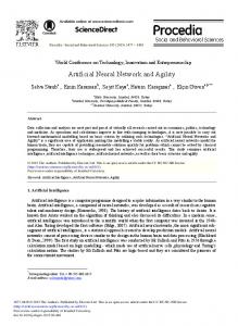
Fig. 1. Haberman data set trained neural network pruning.

Fig. 2. Monks2 data set trained neural network pruning.

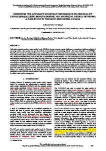
Fig. 3. WDBC data set trained neural network pruning.

Fig. 4. Ionosphere data set trained neural network pruning.

135 Unauthenticated Download Date | 9/23/15 4:20 PM

Information Technology and Management Science ___________________________________________________________________________________________________________ 2014 / 17

vector of weights for the arcs connecting the input layer and the m-th hidden unit, m = 1, 2, …, h. vm is a C-dimensional vector for the weight connecting the m-th hidden unit and the output layer. The activation function is a sigmoid function with domain (−1, +1):

 ( y) 

1 1  e y

effects of pruning. In cases when a train error rises significantly – a neuron is not pruned. All in all, training set classification graphs show decrease of train set classification error. V. DISCUSSION

(5)

Finally, for all our weights we applied weight decay factor 0.0001. This is a quite simple approach in comparison with others described in the theoretical part, but still it does the job. Cross-entropy has been chosen as it is capable of dealing with problems of error derivative plateau better than a standard round mean square error (RMSE) [25]. Apart from this, we used Stochastic Gradient Descent batch training. Batch size was chosen to be 20. IV. EXPERIMENTS In our experiments, we used three 10-fold cross-validation, but for some test-sets like monk’s train and test data are already provided; thus, there we utilized thirty runs to get averaged results. We decided to use two hidden layer neural networks, so that some networks would be able to use an additional layer, in case one of the layers was not needed we would be able to see this after pruning would be finished – such layers should have small number of intact neurons in one of the layers. For our experiments, we used well- known UCI [24] data sets: Monks-1, Monks-2, Monks-3, Ionosphere, Haberman, Pima diabetes, WDBC, WPBC and Parkinsons. Some of the mentioned problems use only categorical variables – like monks. In such cases, we transformed input data into binary format, thus instead of 5 inputs we used 17. In other cases, the only transformation applied was rescaling of data into [−1, 1] region. Data sets are binary classification problems; we utilized two output neurons to represent a solution to the network. Data sets themselves are pretty small ranging from about 150 to 500 entries. Table I holds classification accuracy for all data sets. It contains average classification rate with standard deviation for both train and test cases along with 10 x-validation folds or runs for nonpruned and pruned neural networks. Last table column holds network hidden layers structures before and after pruning. For the pruning algorithm we used 0.025 as an errorRiseTol tolerance level, usually around 50 (depends on the total number of neurons, it should be around 60–70 % of that) as maxIter iterations. MaxIter count should be larger than the maximum number of neurons to be pruned (which was always equal to neuron count in hidden layers minus 2 – we could not prune all neurons from all layers). In all cases, we decided to apply 2 layer hidden neuron networks (with errorbackpropagation) trained using cross-entropy cost (error) function and stochastic gradient descent as a learning algorithm. All cases were executed using 10-fold crossvalidation except monk’s data sets – they had already been divided into training and testing sets. Figs. 1–4 represent a pruning process. Looking at a crossentropy train error one can notice spikes upon neuron removal. In majority of cases, a network is rather quickly adapting to

As one can notice in many cases the acquired ANN models are significantly smaller than initial networks. Smaller networks are less prone to overfitting, thus have higher generalization abilities. In some cases, networks were not significantly simplified; these were: WDBC and Parkinsons data sets, where we could see only ~50 % drop in neuron counts. Both of these data sets have a rather complex structure and thus require bigger models (in comparison with other data sets). As we have already noted, the algorithm has autostopping criteria allowing it to perform several trials before deciding to stop. The used algorithm assumes training of neural network with the removed neuron, while afterwards in case of unsatisfactory results the removed neuron is returned back to the ANN. Diligent reader can note that there are several possibilities in regards to how and which neuron should be returned back into a neural net. We used the same neuron, but we did not explore possibilities of adding a random neuron. VI. CONCLUSION In the current paper, we presented the algorithm for pruning artificial neural networks along with experimental data (UCI classification data sets were used), showing that it was able to significantly simplify a network structure, if a data set did not have a complex structure. Algorithm with the proposed stopping criteria applied to UCI datasets in many cases is giving much simpler ANN models with only a few neurons while having slightly worse or in some cases better classification accuracy rates in comparison with original nonpruned neural networks. Such “simpler” models are faster to execute and are better candidates for knowledge extraction. Further research directions are exploration of other techniques for returning a neuron back after a retraining phase. REFERENCES [1]

[2]

[3]

[4]

[5]

[6]

A.-Krizhevsky, I. Sutskever, G. Hinton. “ImageNet Classification with Deep Convolutional Neural Networks”, Advances in Neural Information Processing Systems 25, NIPS, 2012. G. Hinton, L. Deong, D. Yu, G. Dahl and others, “Deep Neural Networks for Accoustic Modelling in Speech Recognition”. IEEE Signal Processing Magazine, Nov., 2012. http://dx.doi.org/10.1109/MSP.2012.2205597 X. Qiang, G. Cheng, Z. Wang, “An Overview of Some Classical Growing Neural Networks and New Developments”, IEEE, Education Technology and Computer (ICETC), 2nd International conference, vol. 3. 2010. V. Chaudhary, A. K. Ahlawat, R. S. Bhatia, “Growing Neural Networks using Soft Competitive Learning”. International Journal of Computer Applications (0975-8887) vol. 21, no. 3, May 2011. R. Reed, “Pruning Algorithms – A Survey”, IEEE Transactions on Neural Networks, vol. 4., no. 5., Sep. 1993. http://dx.doi.org/10.1109/72.248452 M. C. Mozer and P. Smolensky, “Skeletonization: A Techique for Trimming the Fat From a Network via Relevance Assessment,” in

136 Unauthenticated Download Date | 9/23/15 4:20 PM

Information Technology and Management Science 2014 / 17 ___________________________________________________________________________________________________________

[7]

[8]

[9] [10]

[11]

[12] [13]

[14]

[15]

[16]

[17]

[18]

[19]

[20]

Advances in Neural Information Processing, pp. 107–115, Denver, 1989. B. E. Segee and M. J. Carter, “Fault Tolerance of Pruned Multilayer Networks,” in Proc. Int. Joint Conf. Neural Networks, vol. 2, Seattle, pp. 447–452, 1991. E. D. Karnin, “A Simple Procedure For Pruning Back-Propagation Trained Neural Networks”, IEEE Trans. Neural Networks, vol. 1., no. 2, pp. 239–242, 1990. http://dx.doi.org/10.1109/72.80236 R. Setiono and H. Liu, “Understanding Neural Networks via Rule Extraction,” IJCAI, 1995. R. Setiono and W. H. Leow, “Pruned Neural Networks for Regression” in PRICAI 2000 Topics in Artificial Intelligence, Lecture Notes in Computer Science, vol. 1886, 2000, pp. 500–509. http://dx.doi.org/10.1007/3-540-44533-1_51 Y. Le Cun, J. S. Denker, and S. A. Solla, “Optimal Brain Damage,” in Advances in Neural Information Processing (2), D. S. Touretzky Ed. (Denver 1989), 1990, pp. 598–605. B. Hassibi, D. G. Stork, G. J Wolf, “Optimal Brain Surgery and General Network Pruning.” Y. Chauvin, “A Back-Propagation Algorithm With Optimal Use of Hidden Units” Advances in Neural Information Processing, (1) D. S. Touretzky ed. (Denver 1998), 1989, pp. 519–526. A. S. Weigend, D. E. Rumelhart, and B. A. Huberman, “BackPropagation, Weight Elimination and Time Series Prediction,” in Proc. 1990 Connectionist Models Summer School, D. Touretzky, J. Elman, T. Sejnowsky, and G. Hinton, Eds., 1990, pp. 105–116. A. S. Weigend, D. E. Rumelhart, and B. A. Huberman, “Generalization by Weight-Elimination Applied to Currency Exchange Rate Prediction,” in Proc. Int. Joint Conf. Neural Networks, vol. I, (Seattle), 1991, pp.837–841. A. S. Weigend, D. E. Rumelhart and B. A. Huberman, “Generalization by Weight-Elimination With Application to Forecasting,” in Advances in Neural Information Processing (3) R. Lippmann, J. Moody, and D. Touretzky, Eds., 1991, pp. 875–882. C. Ji, R. R. Snapp, and D. Psaltis, “Generalizing Smoothness Constraints From Discreet Samples,” Neural Computation, vol. 2, no. 2, 1990, pp. 188–197. http://dx.doi.org/10.1162/neco.1990.2.2.188 D. C. Plaut, S. J. Nowlan, and G. E. Hinton, “Experiments on Learning by Back Propagation,” Tech. Rep. CMU-CS-86-126, Carnegie Mellon Univ., 1986. S. J. Nowlan, and G. E. Hinton, “Simplifying Neural Networks by Soft Weight-Sharing,” Neural Computation vol. 4, no. 4, 1992, pp. 473–493. http://dx.doi.org/10.1162/neco.1992.4.4.473 L. Prechelt, “Adaptive Parameter Prunning in Neural Networks,” International Computer Science Institute, Mar. 1995.

[21] W. Finnoff, F. Hergert, and H. G. Zimmermann, “Improving Model Selection by Nonconvergent Methods”, Elsiever Neural Networks, vol. 6, no. 6, 1993, pp. 771–783. http://dx.doi.org/10.1016/S0893-6080(05)80122-4 [22] J. K. Kruschke, “Creating Local and Distributed Bottlenecks in Hidden Layers of Back-Propagation Networks,” in Proc. 1988 Connectionist Models Summer School, D. Touretzky, G. E. Hinton, and T. Sejnowsky, Eds., 1988, pp 120–126. [23] J. K. Kruschke, “Improving Generalization in Back-Propagation Networks with Distributed Bottlenecks,” in Proc. Int. Joint Conf. Neural Networks, Washington DC, vol. 1, 1989, pp.443–447. [24] K. Bache, M. Lichman, (2013), UCI Machine Learning Repository [Online]. Available: http://archive.ics.uci.edu/ml, Irvine, CA: University of California, School of Information and Computer Science. Accessed Sept 15, 2014. [25] P. Golik, P. Doetsch, and H. Ney, “Cross-Entropy vs. Squared Error Training: a Theoretical and Experimental Comparison”, in Interspeech, pp. 1756–1760, Lyon, France, August 2013. Andrey Bondarenko received the B.Sc. degree in 2004, and MSc. degree in 2006 from the Institute of Transport and Communication, University of Latvia, (Riga, Latvia). Since 2010 he has continued studies at Riga Technical University towards obtaining of the Doctoral degree in Computer Science. Presently his major field of study is the extraction of concise rules from a trained artificial neural network. His research interests include: computational intelligence, machine learning. E-mail: [email protected]. Arkady Borisov received the Doctoral degree in Technical Cybernetics from Riga Polytechnic Institute in 1970 and Dr. habil. sc. comp. degree in Technical Cybernetics from Taganrog State Radio Engineering University in 1986. He is a Professor of Computer Science with the Faculty of Computer Science and Information Technology, Riga Technical University. His research interests include fuzzy sets, fuzzy logic, computational intelligence and bioinformatics. He has more than 235 publications in the field. He is a member of IFSA European Fuzzy System Working Group, Russian Fuzzy System and Soft Computing Association, honorary member of the Scientific Board, member of the Scientific Advisory Board of the Fuzzy Initiative Nordrhein-Westfalen (Dortmund, Germany). Address: 1 Kalku Str., Riga, LV-1658; phone: +371 6708953 E-mail: [email protected].

Andrejs Bondarenko, Arkadijs Borisovs. Mākslīgo neironu tīklu vispārināšana un vienkāršošana, izmantojot samazināšanu Šobrīd mēs piedzīvojam otro mākslīgo neironu tīklu (MNT) renesansi. Iemesls – veiksmes apmācības nozarē. Pašlaik kļuvis iespējams apmācīt daudzslāņu tīklus, izmantojot lielus datu apjomus. Tomēr, tāpat kā iepriekš, MNT izmantošanu ierobežo tas, ka dotais modelis ir melna kaste, kura nepaskaidro, kā notiek klasifikācija, kādi faktori un kādā veidā ietekmē klasifikācijas rezultātu. Vēl viena problēma, izmantojot MNT, ir tīkla hiperparametru atlase. Viens no tiem − tīkla arhitektūra ievērojami ietekmē MNT vispārināšanas iespējas. Lai zināšanas izvilktu no tīkla (likumu iegūšana) un vienkāršotu tīklu, kā arī lai palielinātu vispārināšanas iespējas, ir divas pieejas: apmācīt ļoti lielu tīklu, un pēc tam to vienkāršot, vai pakāpeniski apmācīt mazu tīklu, palielinot neironu skaitu. Šis raksts sniedz pārskatu par MNT samazināšanas metodēm. Ir dots pārskats par šādām samazināšanas metodes klasēm: jutīguma analīzes metode, neironu svaru soda metode, neironu svaru pakāpeniska samazināšana, interaktīva samazināšana, automātiska samazināšana u. c. Šajā rakstā tiek ierosināts un apskatīts algoritms, kurš samazina tīklu. Testiem ir izmantoti dati no UCI glabātuves. Metode balstās uz neironu izņemšanu un, ja vajag, atdošanu tīklā. Izmantotais neironu tīkls − daudzslāņu perceptrons − apmācīts svaru samazināšanai. Algoritmam ir automātiskās apstāšanās kritērijs. Iegūtie rezultāti liecina, ka atkarībā no datu sarežģītības, samazinātais un vienkāršotais MNT var būt ievērojami mazāks un vispārīgāks, nekā oriģinālais tīkls. Bieži vienkāršošana samazina klasifikācijas kļūdu. Iegūtais MNT visos gadījumos ir mazāks par oriģināliem tīkliem un to var izmantot noteikumu iegūšanai. Андрей Бондаренко, Аркадий Борисов. Обобщение и упрощение искусственных нейронных сетей через урезание В данный момент мы наблюдаем второй ренессанс искусственных нейронных сетей (ИНС). Причина этого - успехи в области глубокого обучения. На данный момент стало возможным обучение многослойных сетей на больших объемах данных. Однако, как и прежде, ограничением к использованию ИНС является то, что данный вид модели является черным ящиком, не дающим объяснения, как проводится классификация и какие факторы и как влияют на результат классификации. Другой проблемой при использовании ИНС является подбор гиперпараметров сети. Один из них – архитектура сети значительно влияет на обобщающие возможности ИНС. Как для формализации модели (извлечение правил), так и для упрощения сети и частично увеличения обобщающих возможностей проводят обучение излишне большой сети с последующим урезанием, либо обучение маленькой сети с последующим добавлением нейронов. В данной статье приведен обзор методов урезания. Рассмотрены такие подходы, как: анализ чувствительности, методы на основе штрафа, методы распада весов нейроных связей, интерактивного урезания, автоурезания и другие. В данной статье предложен и рассмотрен алгоритм урезания сети на примере данных из UCI репозитория на основе удаления и, по необходимости, возврата нейронов в сеть. Нейронная сеть – многослойный персептрон, обученный при помощи обратного распространения ошибки. Алгоритм обладает критерием остановки. Полученные результаты говорят о том, что в зависимости от сложности данных модель ИНС может быть значительно упрощена и обобщена. Зачастую урезание уменьшает классификационную ошибку. Полученные ИНС во всех случаях становятся меньше оригинальной сети и могут быть использованы для извлечения правил.

137 Unauthenticated Download Date | 9/23/15 4:20 PM