Chulan Kwon, Youngah Park. Department of Physics, Myong Ji University, Yongin, Kyonggi, Korea. (January 10, 1993). Abstract. Learning of a fully connected ...
Generalization in a two-layer neural network
Kukjin Kang, Jong-Hoon Oh Department of Physics, Pohang Institute of Science and Technology, Pohang, Kyongbuk, Korea
Chulan Kwon, Youngah Park Department of Physics, Myong Ji University, Yongin, Kyonggi, Korea
(January 10, 1993)
Abstract Learning of a fully connected two-layer neural networks with N input nodes, M hidden nodes and a single output node is studied using the annealed ap-
proximation. We study the generalization curve, i.e. the average generalization error as a function of the number of the examples. When the number of examples is the order of N , the generalization error is rapidly decreasing and the system is in a permutation symmetric(PS) phase. As the number of examples P grows to the order of MN the generalization error converges to a constant value. Finally the system undergoes a rst order phase transition to a perfect learning and the permutation symmetry breaks. The computer simulations show a good agreement with analytic results. 87.10.+e, 05.50.+s, 64.60.Cn
Typeset using REVTEX 1
Following the pioneering works of Gardner [1,2], there have been many e�orts [3{6] to apply the methods of statistical mechanics to understand the feed-forward neural networks such as a perceptron [7]. Two main issues were studied in this context. Gardner studied the storage capacity of the single layer perceptron and there are several works in the same line [1{3]. The other problem is the learning curve, which shows a variation of the average error as a function of the number of training examples. For the single layer perceptron, this problem was studied extensively using the statistical mechanics [4{6,8,9] and also using the mathematical approach [10]. However, it is well known that the perceptron architecture can only solve a linear threshold problem. Many of the real-world problems are approached using the networks with a hidden layer and the error back-propagation algorithm [11]. Usually, direct application of the error-back-propagation algorithm has problems such as a large computing time required for learning and the existence of many local minima which prevents proper learning. Also estimation of an appropriate size of training example set for a valid generalization is an important issue. Study of generalization curve can give many useful information for such problems. However, existence of the hidden layer makes learning mechanism much more complex than that of single layer perceptron and not much is known about the generalization of multi-layer networks. Tree like architecture where an input node is connected to only one hidden node was studied by several groups [12{14]. Recently there have been some e�orts to get the storage capacity of fully connected two-layer networks [15,16]. Here we present a study of the generalization curve of a fully connected two-layer network which is believed to perform a fairly complex task. Consider a two-layer feed-forward network with N input nodes, M hidden nodes and a single output node. Every input node is connected to all of the hidden nodes by the binary weights. Specially, we set all the weights in the second layer to 1. This architecture is usually called the committee machine. Suppose we have a network with arbitrary binary weights, we can always map this network into a committee machine by changing the sign of weights in the second layer which are ?1 and the signs of all the weights in the rst layer connected to those negative weights. When the 2
transfer function is an odd function, this new network performs exactly the same function as the original one. We calculated the generalization curve for this machine using the annealed approximation. When the number of examples is the order of N , the generalization error is rapidly decreasing and the system is in a PS phase which we will explain below. When the number of examples P grows the order of MN the generalization error converges to a constant value and does not decrease until a rst order phase transition to a perfect learning is reached. Above the transition the permutation symmetry breaks. The Monte Carlo simulations of the networks with various transfer functions well agree with the annealed calculations. Using the permutation symmetry property, we are able to calculate the generalization curve using the similar method used for a perceptron learning. The network maps input vector S l = fSil; : : : ; SNl g to output � as � (W ; S l ) = g2 (M ? 2 1
M X j
g1 (N ? 2 1
N X i
Wji Sil )):
(1)
W = fWji g is a set of the synaptic weights whose element Wji is a weight from the ith input node to the j th hidden node. g1 (x) and g2(x) are transfer functions of the hidden layer neuron and the output neuron respectively. A teacher network has the same architecture as that of the student. The weights of the teacher are given by W 0 = fWji0 g. The training procedure is a Glauber dynamics which leads at long times to a Gibbs distribution of the weights. Energy of the system is de ned as follows. E=
P X l=1
�(W ; S l );
(2)
1 (3) 2 The performance of the network is measured by the generalization function �(W ) = R R dS �(W ; S ), where dS represents an average over the whole space of inputs. The generalization error �g is de ned by �g = hhh�(W )iT ii where hh� � �ii denotes the quenched average over the examples and h� � �iT is the thermal average. An input Sil is chosen according to a Gaussian distribution with variance unity. �(W ; S l ) = [� (W 0 ; S l ) ? � (W ; S l )]2:
3
In this letter, we will rely on the annealed approximation. Actually from our preliminary result using the replica trick, we have a con dence that most of the qualitative behavior of the network is explained within the annealed calculation. Also it was known from the study of single layer perceptron that the annealed calculation gives a pretty good quantitative prediction of the generalization curve [5]. So, we replace the quenched average of the free energy with the annealed average,
? F = hhln Z ii ' lnhhZ ii:
(4)
Here = 1=T in which the temperature T parametrizes the level of stochastic noise. The free energy depends on the overlap order parameter matrices R; Q de ned as follows. Rjk =
1
N
N X i
Wji Wki0 ;
N X 1 Wji Wki : Qjk = N
(5)
i
An interesting property of this fully connected machine is that by exchanging positions of two hidden nodes we can construct another network which performs an equivalent task as the original network does. We might expect that the student has a close correlation with one of the networks constructed by the permutation of the teacher network. We assume this asymmetry makes diagonal elements of the matrix have di�erent value with the rest of the matrix elements. Qjk = �jk + (1 ? �jk )Q;
Rjk = �jk R1 + (1 ? �jk )R0 :
(6)
Also we assume the teacher does not have any correlation between sites, i.e. P N ?1 Ni Wji0 Wki0 = �jk : In the thermodynamic limit where M and N go to in nity, we can use the saddle point analysis for the free energy. Then the saddle point solution gives the order parameters Q; R0; R1. As the order of magnitude of the number of examples varies, the free energy and the order parameters scale di�erently. We consider three di�erent cases, where P is of the order of N , MN and in the intermediate region. We present the results 4
for the cases where transfer functions are sign(x), x. Our method can also be applied to other transfer functions. 1. P � O(N ): The free energy can be divided into the entropy part G0 and Gan = lnhhe? �ii,
? F = N (G0 + �Gan ):
(7)
Here the number of examples P scales as � = P=N . G0 and Gan are the order of unity. We nd an important result, 1 (8) R = R � O( ): 0
1
M
This condition corresponds to the so called permutation symmetry pointed out by Barkai et al. [15] To show this, we calculated G0 and Gan up to the order of 1=M . Note that the permutation of the hidden nodes of a given teacher yields many networks which give equivalent outputs. Each of the permuted networks becomes an equivalent teacher. Let us consider the energy surface in the phase space fW g. Each teacher is at a minimum of the energy surface. For a small number of examples P and a high temperature T , all the teachers belong to a single thermally connected region in the phase space. In this case, a student does not know from which teacher to learn, and the student is roughly in a equi-distance from all of the permuted teachers. This picture coincide with the permutation symmetry described by Eq. (8). The learning rate is also relatively fast. For a large P and a low T , there appear many thermally disconnected valleys around the permuted teachers. In this case, the permutation symmetry is broken, which will be discussed in the case 2. In this PS phase, the free energy and the generalization error �g is given as 1 1 (9) G0 = ? Q� + ln(1 ? R� 21 + Q� ); 2 82 > > < ? 1 ln(1 + 2 �g ); g2 (x) = x Gan = > 2 : (10) > : ln(1 + e?22 ?1 �g ); g2 (x) = sign(x) 8 > > � �1�22 + �222 Q; < �1 ? R g2 (x) = x � � : (11) �g = > 2 2� > : � cos?1 p 2�2R1 2 � ; g2 (x) = sign(x) � +�1 � Q 1
2
5
R
R
1 Dx [g (x)]2, � = 1 Dx x g (x) where Dx = pdx e? 21 x2 . We rescaled the We de ne �1 = ?1 1 2 1 ?1 2� order parameters as R� 1 = MR1 and Q� = MQ. When � goes to in nity, the generalization error converges to a limit �0. 8 > > < �1 ? �22 ; �0 = > � > ?1 :2 � cos
p��2
�
1
g2 (x) = x ; g2 (x) = sign(x)
(12)
:
When �1 = �22, �0 becomes zero. A network with g1(x) = x belongs to this case. Here, the permutation symmetry holds for all values of P . A network with a linear transfer function in the rst layer maps to a single layer perceptron with continuous weights. E�ective weight of this perceptron from i-th input node is M ?1=2 PMj Wji for a student and M ?1=2 PMj Wji0 for a teacher. In the limit M goes to in nity, the e�ective weights become continuous. The e�ective weights of all the permuted teachers are the same. The generalization error decays with an asymptotic form �g / 1=�. This explains why learning of the two layer network with a linear transfer function in the hidden layer shows the same asymptotic behavior as that of a single layer perceptron with continuous weights [5]. Generally, �0 is non-zero for a non-linear g1(x), which means learning is not fully accomplished in the region P � N . 2. P � O(MN ): In this case we introduce a new scaling for the free energy,
? F = MN (G0 + �0Gan );
(13)
where �0 = P=MN . G0 and �g are given by 1 2
1 2
G0 = ? (1 + R1 ) ln(1 + R1 ) ? (1 ? R1 ) ln(1 ? R1 );
�g
8 > > < �1 ? �3 ? (1 ? R1 )�22 ; � �r => 2 ?1 (�3?R1 �22 )2 +(�1 ?�22 )�22 > : �
cos
�1 (�1 ?�22 )
q
g2 (x) = x ; g2 (x) = sign(x)
;
(14) (15)
1 R 1 DxDy g ( 1 ? R2 x + R y )g (y ). G has the same form as in Eq. (10). where �3 = R?1 1 1 an 1 1 ?1 The other order parameters are eliminated by the saddle point condition. For a network with a nonlinear transfer function in the hidden layer, there are two solutions for R1. One is the PS solution, where R1 = 0 and �g is equal to �0 of Eq. (12).
6
This corresponds to the limit where � goes to in nity in the case 1. The other is the permutation symmetry breaking(PSB) solution where R1 is non-zero. When either g1(x) or g2(x) is the sign function, R1 is one and �g is zero. This solution can be interpreted as a perfect learning state. When both transfer functions are continuous, we have small �g decaying exponentially for large �0 . There is a rst order phase transition from the PS phase to the PSB one. The transition line �0c (T ) is determined by comparing the free energy of the two solutions. For g1(x) = sign(x) and g2(x) = x, �0c(T ) / ?1= ln T at low T . For g1 (x) = g2 (x) = sign(x), �0c (T ) ? �0c (0) / e?2=T and �0c (0) ' 1:3. It can be shown that the PS solution exists in the whole �0-T plane. Therefore it is very di�cult to observe the transition from the simulation if the network is a fairly large size. For a network with smaller size, M = N = 10, we observed the transition from the the Monte Carlo simulation. 3. Intermediate region. P � M � N : In this region, we studied the network whose transfer function is the sign function for both layers. Note that the order parameters R�1 and Q� diverge as P=N goes to in nity. We examined this divergence in detail for 0 < � < 1. As a result, we nd R1 and Q scale as R1 = R0 / M ?
Q / M?
?
2 � 2
?
4 � 4
:
(16)
For large M , R1 goes to zero, which leads to the PS solution discussed in the case 2. The learning curve from the annealed calculation is compared with the Monte Carlo simulation. Fig. 1 shows the learning curve for the case g1(x) = g2(x) = sign(x). Fig. 2 shows the learning curve for the case g1(x) = g2(x) = tanh x. For the latter case, the free energy and the generalization error do not have a closed form as above. We nd the saddle point and the generalization error numerically. The simulation results show a pretty good agreement with the annealed calculations. The limiting value �0 of the generalization error is much smaller for the transfer function tanh(x). With a smother hidden layer transfer function, we obtain a smaller �0 and a larger �0c . There are some e�orts to derive an asymptotic behavior of the learning curve by analyzing the scaling of the volume of solution space [17,18]. These approach is usually useful for a 7
network with continuous weights. The generalization error for a machine with continuous weights is inversely proportional to the ratio of training examples and the number of weights in the network. If we apply this theorem to the two-layer machine with continuous weights, the generalization error should decay with a 1=�0 form. However, in the PS phase the permutation symmetrycondition which is not considered in this theorem reduces the e�ective number of weights to the order of N . This explain a rather fast decay of the error with a power law 1=� in the region P � N . As the number of example P grows to the order of MN , the permutation symmetry breaks and the asymptotic behavior of the learning curve in the PSB phase slows down to the scale 1=�0 . This expectation does agree with the result by Schwarze and Hertz [19] and also with our calculation not reported here. For binary weights we are dealing with here, the asymptotic behavior is similar in the PS phase. A combination of M binary weights behaves like a continuous weight. In the PSB region, binary weights a�ect the asymptotic behavior signi cantly. The asymptotic decay after the transition is not observed for most of the networks with sigmoidal transfer functions. Summarizing our results, learning from examples in this fully connected two-layer network has an intrinsic limitation due to the existence of the metastable PS state above the thermodynamic transition. If the system has moderately large size, the system is trapped to the the metastable state in most cases. The minimum generalization error we have in the PS state critically depends on the form of the transfer function. Many of the e�orts to improve the back-propagation network were concentrated on the development of better learning algorithm with fast convergence without consideration of the energy surface structure of the system. Our result shows that a more e�ective way for improvement is to analyze the phase space structure and to nd an optimal architecture of the network with appropriate transfer functions. It may be useful to nd an energy function which has less local minimum than the usual quadratic form [20]. Other approach where the network is constructed by adding hidden nodes during the training may be helpful to avoid the local minima [21,22]. We appreciate H. Schwarze for sending the preprint prior to publication. During the progress of this work [23] we came to know that they were doing the similar calculation for 8
the case where the transfer functions are sign function. This work was supported in part by the KOSEF through the Center for Advanced Materials Physics at POSTECH and the Center for Theoretical Physics of Seoul National University. It is also supported by the Basic Science Research Institute of POSTECH. K. K. and J. H. O. appreciate nancial support from RIST.
9
REFERENCES [1] E. Gardner, Europhys. Lett. 4, 481 (1987); J. Phys. A 21, 257 (1988). [2] E. Gardner and B. Derrida, J. Phys. A 22,1983 (1989). [3] W. Krauth and M. M�ezard, J. Phys. (Paris) 50, 3057 (1989). [4] H. Sompolinsky, N. Tishby, and H. S. Seung, Phys. Rev. Lett. 65, 1683 (1990). [5] H. S. Seung, H. Sompolinsky, and N. Tishby, Phys. Rev. A 45, 6056 (1992). [6] G. Gyorgyi, Phys. Rev. Lett. 64, 2957 (1990); Phys. Rev. A 41, 7097 (1990). [7] M. L. Minsky and S. Papert, Perceptron (MIT Press, Cambridge , MA, 1969). [8] K. Kang, J.-H. Oh, C. Kwon, Y. Park, and H. S. Song, J. Kor. Phys. Soc. 25, 270 (1992). [9] C. Kwon, Y. Park, and J.-H. Oh, Phys. Rev. E, in press. [10] S. Amari, N. Fujita, and S. Shinomoto, Neural Comput. 4, 605 (1992). [11] D.E. Rumelhart, G. E. Hinton, and R. J. Williams, in Parallel Distributed Processing: Explorations in the Microstructure of Cognition, edited by D.E. Rumelhart and J. L. McClelland, (MIT Press, Cambridge, MA, 1986) Vol. 2, pp 318-362. [12] M. Opper and D. Haussler, Phys. Rev. Lett. 66, 2677 (1991). [13] H. Schwarze, M. Opper and W. Kinzel, preprint (1992). [14] G. Mato and N. Parga, J. Phys. A 25, 5047 (1992). [15] E. Barkai, D. Hansel and H. Sompolinsky, Phys. Rev. 45, 4146 (1992). [16] A. Engel, H. M. Kohler, F. Tschepke, H. Vollmayr, and A. Zippelius, Phys. Rev. A 45, 7590 (1992). [17] S. Amari, preprint (1992). 10
[18] H. S. Seung, M. Opper, and H. Sompolinsky, Proceedings of the Fifth ACM Workshop on Computational Learning Theory, (ACM, New York, 1992) pp 287-294. [19] H. Schwarze and J. Hertz, preprint (1992). [20] E. Eisenstein and I. Kanter, preprint (1992). [21] P. Rujan and M. Marchand, Complex Systems 3, 229 (1989). [22] M. Biehl and M. Opper, Phys. Rev. A 44, 6888 (1991). [23] K. Kang and J.-H. Oh, in the presentation at The 18th IUPAP International Conference on Statistical Physics, Berlin, August 2-8, 1992.
11
FIGURES
1
.8
.6
.4
.2
0 0
100
200
300
FIG. 1. Generalization curve for a network with the transfer functions g1(x) = g2(x) = sign(x), N = M = 31, and the temperature T = 5. The solid line is the analytic plot from the annealed
approximation and the horizontal line denotes �0 . The rst order transition at �0c ' 9:9 is shown with the vertical dashed line. Dots show the result from the Monte Carlo simulation.
12
1
.8
.6
.4
.2
0 0
50
100
150
FIG. 2. Generalization curve for a network with the transfer functions g1(x) = g2 (x) = tanh x, N = M = 31, and the temperature T = 5. The solid line is the analytic plot from the annealed
approximation and the horizontal line denotes �0 . Dots show the result from the Monte Carlo simulation. �0c ' 207 is too large to be shown in this graph.
13