04JEI00038 1726-2135/1684-8799 © 2004 ISEIS www.iseis.org/jei
Journal of Environmental Informatics 4 (2) 65-74 (2004)
Artificial Neural Networks Application in Lake Water Quality Estimation Using Satellite Imagery S. S. Panda, V. Garg and I. Chaubey1* Biological and Agricultural Engineering Department, 203 Engineering Hall, University of Arkansas, Fayetteville, AR 72701 ABSTRACT. Lake water quality monitoring using traditional water sampling and laboratory analyses is very expensive and time consuming. Application of neural networks to predict water quality using satellite imagery data has a potential to make the water quality determination process cost-effective, quick, and feasible. This paper includes an indirect method of determining the concentrations of chlorophyll-a (chl-a) and suspended matter (SM), two optically active parameters of lake water quality. Radial basis function neural (RBFN) network models are developed to predict the chl-a and SM concentrations in the lake. The low cost commercially available Landsat-TM imagery spectral information was used as the input with chl-a or SM concentrations as output. The model is trained and validated with data from the years 2001, 2002, 2003, and 2004. The model testing resulted in a coefficient of determination (R2) of 0.55 and 0.90, respectively, for actual and predicted chl-a and SM concentrations. The root mean square error (RMSE), standard error of prediction (SEP), and average testing accuracy indicated the merit of the developed models. Keywords: Chlorophyll, image processing, RBFN, remote sensing, suspended matter
1. Introduction Accurate quantification of lake water quality is essential for its management and improvement. Traditionally, lake water quality assessment has been limited to in-situ collection and measurement of water samples for subsequent laboratory analyses – a method that is accurate but expensive and time consuming. Time and cost constraints associated with in-situ measurements of lake water quality often limit assessment of spatial and temporal trends of water quality. Remote sensing has a potential to overcome these constraints by providing an alternative means of water quality monitoring over a greater range of temporal and spatial scales (Dekker et al., 1996). In addition, remote sensing can be used as a valuable tool to retrieve water quality information of ungauged lakes from a vast amount of archived remote sensing data. Chlorophyll-a (chl-a), suspended matter (SM), and dissolved organic matters are optically active parameters of lake water quality. Several investigators have successfully used Landsat-MSS/TM imagery in inland and estuarine water quality monitoring (e.g., Ritchie et al., 1990; Lathrop, 1992; Choubey, 1994; Keiner and Yan, 1998; Brivio et al., 2001; Baruah et al., 2001; Wang and Ma, 2001). In case of inland water, the water dynamics is more complex to have a linear relationship between the satellite spectral signatures and the water quality parameters. There is considerable scattering (in all visible and even in near-IR bands) from the lake waters with high sediment and chlorophyll content (Baruah et al., 2001). * Corresponding author:
[email protected]
For nonlinear environmental processes, artificial neural networks (ANN) could be used due to its ability in modeling nonlinear geophysical transfer functions. A neural network is a parallel-distributed processor that has a natural property for storing experimental knowledge and making it available for use (Haykin, 1999). Through learning procedures, ANNs have the power to approximate any non-linear relationship that exists between a set of inputs and their corresponding set of outputs (Lacroix et al., 1997). Artificial neural networks have the ability of computing, processing, predicting and classifying data and have the advantages of nonlinearity, input-output mapping, adaptivity, generalization, and fault tolerance (Haykin, 1999). The ANN techniques are based on the configuration of several prediction, classification, and time series estimation techniques. Zhuang and Engel (1990), Ranaweera et al. (1995), and Panda and Panigrahi (2000) have provided research evidences regarding the superiority of ANN modeling technique over the statistical process in the case of nonlinear data modeling. Keiner and Yan (1998), and Baruah et al. (2001) have established the importance of backpropagation neural networks (BPNN) over the multiple regression technique while predicting water quality from satellite imagery. The ANN models provided R2 of 0.94 for the chl-a versus Landsat TM spectral information (Keiner and Yan, 1998). Baruah et al. (2001) encountered a significant increase in R2 with their ANN models of chl-a versus Landsat-TM. The authors reported R2 of 0.31 with statistical regression model and improved R2 of 0.93 with the ANN model. Radial basis function network (RBFN) methodology has found increased application in pattern recognition, signal
65
S. S. Panda et al. / Journal of Environmental Informatics 4 (2) 65 - 74 (2004)
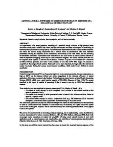
processing, load forecasting, and crop prediction modeling, etc., due to its structural simplicity and training efficiency (Goodman, 1993; Ranaweera et al., 1995; Walczak and Massart, 1996; Lee et al., 1996; Wan and Harrington, 1999; Panda et al., 2002). The RBFN architecture is different from some other neural networks such as back-propagation neural networks (BPNN). The RBFNs have certain advantages over the BPNN such as guaranteed learning algorithm (e.g., linear least squares optimization) (Walczak and Massart, 1996). Application of RBFN modeling in quantifying lake water quality has not been done in the past. The objective of this study was to develop and compare RBFN model with a statistical model to predict chl-a and SM concentration using the Landsat-TM satellite imagery and simultaneously in-situ analyzed spatially distributed water samples from Beaver Reservoir. A typical RBFN consists of three different layers with each successive layer fully connected by feed forward arcs (Moody and Darken, 1989) (Figure 1). There is no provision of weight between the input layer and the hidden layer (prototype). The transfer function used at the hidden layer is the “radial basis functions,” a nonlinear transfer function. Unlike BPNN, there is only one hidden layer present in the RBFN architecture which makes the RBFN model computation faster. Other hidden layers can be used in the RBFN architecture to perform the error back-propagation function. However, these layers are optional and generally not used. The output layer in RBFN is linear (Haykin, 1999). There is an extra prototype layer in the RBFN architecture, where the input vectors after being multiplied with random weights are clustered into different homogeneous groups. The clustered centroids are fed to the prediction model for output prediction (Haykin, 1999). Many complex classification and prediction problems, such as image classification, character recognition, speech recognition, volatile compound detection, and prediction from electronic-nose experiments, have been successfully conducted using RBFNs (Wan and Harrington, 1999). According to Walczak and Massart (1996), RBFNs have certain advantages over the multi-layer perception networks (MLPs) such as BPNN. Contrary to MLP, RBFNs have a guaranteed learning algorithm, e.g., linear least squares optimization. In addition, a common difference between BPNN and RBFN is that a BPNN uses the stochastic approximation as model optimization method whereas the RBFN uses the curve-fitting approximation in a high-dimensional space to obtain a best fit to the training data (Haykin, 1994). In RBFN, the activation function in the hidden units calculates the distance between the input vector and the center of the hidden unit using Euclidean norm. However, MLP uses a scalar product of the input vector and synaptic weight vector of that hidden unit. The distance measurement is efficient in RBFN (Simard et al., 1993). RBFN uses exponentially decaying nonlinear (Gaussian) functions to construct local approximations to non-linear input-output mapping whereas the MLP can only construct a global approximation to non-linear input-output mapping. Localized approximation in input-output mapping is always preferred (Haykin, 1999). The RBFN is an ideal tool for environmental application problems
66
because local approximation of nonlinear input-output mapping results in the RBFN models of fast learning with reduced sensitivity (Haykins, 1999; Hassoun, 1995). Walczak and Massart (1996) also suggested that net convergence is not guaranteed in MLP network, while this problem does not exist in RBFN. Therefore, despite its computational intensity (because the network’s use of high-dimensional space) and its optimal parameterization problem RBFN is currently getting wider recognition.
2. Methodology The study was conducted in the Beaver Reservoir located in NAD 83 UTM coordinates of 389237.20 to 449127.16 m N and 3952318.95 to 4038348.33 m E (Figure 2). Beaver Reservoir is the primary drinking water source for more than 280,000 people in Northwest Arkansas. Northwest Arkansas is among the most rapidly growing metropolitan areas in the US. Eutrophication of the lake is a great concern for long-term Beaver Reservoir water quality management. 2.1. Image and Water Quality Data Acquisition Ten Thematic Mapper (TM) cloud free images from two Path/Row combinations (25/35 and 26/35) covering Beaver Reservoir were used in this study (Table 1). The TM images were precision corrected including radiometric and geometric corrections. Six spectral bands: band 1 (TM1), 0.45 – 0.52 µm; band 2 (TM2), 0.52 – 0.60 µm; band 3 (TM3), 0.63 – 0.69 µm; band 4 (TM4), 0.76 – 0.90 µm; band 5 (TM5), 1.55 – 1.75 µm; and band 7 (TM7), 2.08 – 2.35 µm of TM were used to determine the chl-a and SM concentrations in water. Band 6 (57 m resolution) was not used because of the image resolution dissimilarity with other bands that were 28.5 m in resolution. Since 2003, water samples were collected on cloud free dates from different spatial positions of Beaver Reservoir coinciding with TM acquisition dates of the Beaver Reservoir scenes. In addition, chl-a measured data of two United States Geological Service (USGS) gaging stations (#07049500 and #07049691) located in the Beaver Reservoir were also used in this study. The TM scenes were acquired coinciding with cloud free sampling dates of USGS gauging station in 2001 and 2002. The spatial positions of each water sample collection points including the USGS gaging stations are shown in Figure 2. Water samples were collected from three depths (surface, 1 m below surface, and 2 m below surface) for each location. For each water sample, 4 L of water was collected and stored in dark on ice until returned to laboratory for analyses. Upon returned to the laboratory 1000 to 1500 ml of each sample was filtered using Gelman GF/C 47-mm filters for chl-a and SM determination. Filters for chl-a extraction were macerated in 5 ml 90% acetone. Extracts were then cleared by centrifugation and analyzed spectrometrically (APHA, 1998). Filters for determination of SM were preweighed. After sample filtration, filters were oven dried at 105 ºC for 24 h and reweighed to determine SM. Average concentrations of chl-a and SM from three depth samples were used for modeling.
S. S. Panda et al. / Journal of Environmental Informatics 4 (2) 65 - 74 (2004)
Input parameters (IPEs)
Output parameters (OPEs)
B-band
Radial basis function
G-band W1 R-band
W2 Chlorophyll-a / SM
W3
NIR-band
Wn
MIR-band MIR-band
Input Layer
Prototype layer
Output Layer
Figure 1. Structure of a typical radial basis function network (RBFN) model.
Gaging Station Locations 07049691: Beaver Lake at the Dam near Eureka Springs 07049500: Beaver Lake at Highway 12 near Rogers
Figure 2. Location of the study area, watershed stream network, USGS gaging stations, and other water sample collection stations in Beaver Lake in northwest Arkansas.
67
S. S. Panda et al. / Journal of Environmental Informatics 4 (2) 65 - 74 (2004)
Table 1. Landsat TM-5 Image Acquisition and the Corresponding Water Sampling Dates Data Water sampling
Image acquisition
Path/Row
# of water sampling points
2001
April 18 June 13 October 16
April 17 June 13 October 19
25/35 26/35 25/35
2 2 2
2002
July 10 July 24
July 9 July 21
26/35 26/35
2 2
2003
July 21 August 6 December 19
July 21 August 7 December 19
25/35 25/35 26/35
10 12 12
2004
February 21 April 4
February 21 April 2
26/35 25/35
11 10
Year
Typical reservoirs have dendrite shape and longer shorelines compared to lakes. Beaver Reservoir also has a dendrite shape (Figure 2) and its width was small at many sampling points. Therefore, we used single pixel gray values instead of a 3 × 3 window values from each water quality sampling to avoid pixels of window falling outside the water body. Single pixel gray values (digital numbers, DN) of the collected water sample spatial position were extracted and used in modeling. Studentized t-test was applied for outlier detection and one outlier sample data point was eliminated from the database. The gray value of the outlier data was exceptionally high for each band of the image as compared to the other digital numbers. Geomatica 9.1 (PCI Geomatics, Richmond Hill, Ontario, Canada) and IDRISI 32.2 (IDRISI Production, Worcester, MA) software were used for image processing. Figure 3 describes the image processing (DN extraction) procedure. 2.2. Input Dataset Three different input data sets were prepared using DN values of different band of TM images. The dataset 1 (DS1) included six DN numbers of band: TM1, TM2, TM3, TM4, TM5, and TM7. In remote sensing many indices are used based on combination of different bands to improve the natural resources predictability and management (Thiam and Eastman, 1999; Yang and Anderson, 2000; Panda et al., 2004). We created eleven indices using various combinations of band TM1, TM2, TM3, TM4, TM5, and TM7. These eleven indices were: (TM1 + TM2 + TM3) / 3, TM1 / TM2, TM1 / TM3, TM2 / TM3, (TM5 + TM7) / 2, (TM4 + TM5 + TM7) / 3, (TM1 - TM3) / (TM1+ TM3), (TM1 - TM2) / (TM1 + TM2), (TM2 - TM3) / (TM2 + TM3), TM2 + TM3, TM4 + TM5 + TM7. These indices were created on the format of band averaging, simple band division, vegetation indices calculation, and selective band summing. The dataset 2 (DS2) used the values of these eleven indices as the input. Third dataset (DS3) was made of 17 input parameters by pooling 6 DN values of data set 1, and 11 indices values of DS2. For RBFN modeling each dataset was scaled down to
68
values between zero and one using min-max scaling option of the software. The equation used for the scaling technique was
X =
X i − X min X max − X min
(1)
where Xi is the value of the raw input variable, X, for the ith training case; Xmax is the maximum value of a training case; and Xmin is minimum value of a training case in the dataset. These three data sets were then used to develop RBFN models using one of the data set as input and either chl-a or SM concentrations as model output. Similarly, these three data sets were used to develop statistical models using least square multiple regression (LMR) with one of the input dataset as independent variables and either chl-a or SM as dependent variables. In case of statistical modeling, individually each band DN was also used to develop regression models with either chl-a or SM concentrations. For chl-a modeling 64 observations were available for analysis. In statistical modeling all 64 observations were used for developing multiple regression equation. However, for RBFN model development, out of the 64 observations 46 were randomly selected as training and rest 18 were selected as testing observations. For SM modeling only 54 observations were available. Statistical model used all 54 observations. In RBFN modeling, 40 observations were randomly selected for model training and the remaining 14 were selected for model testing. 2.3. RBFN Network Architecture Figure 4 represents the methods used for the image processing to prepare data for the RBFN model building. A typical RBFN model consists of three different layers with each successive layer fully connected by feed forward arcs as shown in Figure 1 (Moody and Darken, 1989). There is no provision of weight between the input layer and the hidden layer (prototype) in the RBFN. A nonlinear transfer function is used at the hidden layer in the RBFN. The output layer in RBFN is linear (Haykin, 1999). The model architecture of RBFN is defined by providing its layer numbers. Figure 1 shows an architecture of 6-5-0-1, which means the network has 6 input neurons/input processing element (IPE), 5 prototype nodes in the prototype layer, zero neurons in the hidden layer for error back-propagation, and 1 output neuron (OPE). We used Neural Ware Professional Plus II software (Neural Ware, Carnegie, PA) for building the RBFN model. For data sets 1, 2, and 3, the RBFN models were constructed with an initial architecture of 6-10-0-1, 11-10-0-1, and 17-10-0-1, respectively. Altogether, six RBFN models were developed; three with chl-a as output neuron and three with SM as output neuron. “Delta rule” as learning rule (Haykin, 1999) and the sigmoid (nonlinear) transfer function were used for model learning. Then, using the procedure outlined in Figure 5, the models were optimized to obtain the best possible prediction model.
S. S. Panda et al. / Journal of Environmental Informatics 4 (2) 65 - 74 (2004)
a) Original TIFF image (single band) of entire
b) Extracted image of only the Beaver Lake
scene with Arkansas State mask
portion
c) Final extracted image single pixel of a particular individual WQ sampling station.
Figure 3. Image extraction process for spectral information collection from Landsat 5 image.
Landsat Image
Transfer of PIX format of images into TIFF
format
Geomatica 9.1
Extraction of individual DN values based on corresponding spatial position
IDRISI macrocode
Arrange the imagery information in a TXT format (use corresponding yield as the last column)
MS-Excel macrocode
Prepare the training and testing file for the RBFN model
Model Building
Figure 4. The procedure followed for image processing and dataset preparation for the RBFN model development.
69
S. S. Panda et al. / Journal of Environmental Informatics 4 (2) 65 - 74 (2004)
For selected parameter of momentum rate and learning rate; vary number of nodes in prototype layer
Determine optimum number of nodes in prototype layer 2
(Based on the lowest MSE/highest R obtained)
Keeping the momentum rate constant with the optimized number of prototype layer nodes; vary the learning rate
Determine the optimum learning rate parameter 2
(Based on the lowest MSE/highest R obtained)
Keeping the learning rate constant with the optimized values of prototype layer nodes; vary the momentum rate
Determine the optimum momentum rate parameter 2
(Based on the lowest MSE/highest R obtained)
Identify the optimum epoch keeping other parameter constant (Based on 2
the lowest MSE/highest R obtained)
Optimum neural network
Figure 5. Schematic of procedure for determining the optimum neural network architecture.
2.4. Statistical Indices for Model Testing The statistical and RBFN model performances were evaluated based on root mean square error (RMSE), prediction accuracy (average test accuracy), standard error of prediction (SEP), and the coefficient of determination (R2). The equation for RMSE is given by
RMSE=
SSE n
(3)
where Y and X are actual and predicted output, respectively. The SEP of the predictive model was calculated by the equation (Kramer, 1998)
(2)
where n is the number of observations; and SSE is sum of squared error. Average test prediction accuracy (ATPA) is calculated by the equation
70
⎛ 1 n Y − Xi ⎞ ATPA = ⎜ 1 − ∑ i ⎟ × 100 ⎝ n i =1 Yi ⎠
n
SEP =
∑ ⎡⎣(Y − X ) − d i =1
i
i
n −1
m
⎤⎦
2
(4)
where dm is mean of the difference between actual and pre-
S. S. Panda et al. / Journal of Environmental Informatics 4 (2) 65 - 74 (2004)
Table 2. Results Obtained from Neural Network and Regression Analysis of RBFN-Chlorophyll-a Prediction Model
Model
Optimal model architecture and parameters (From neural network analysis) Net la Mb Iterations RMSEc
Actual-Predicted model correlation (From regression Average analysis) prediction accuracy (%) αd βe R2f SEPg (µ gm/l) RMSEc (µ gm/l)
Training Testing
6-20-0-1 6-20-0-1
55.37 74.85
0.9 0.9
0.7 0.7
40,000 40,000
0.1713 0.0772
1.00 0.86
-0.15 0.50
0.45 0.55
2.08 1.03
2.06 1.00
Note: a Learning rate coefficient; b Momentum coefficient; c Root mean square error; d Intercept; e Slope; f Coefficient of determination; and g Standard error of prediction.
Table 3. Results Obtained from Neural Network and Regression Analysis of RBFN-SM Prediction Model
Model
Optimal model architecture and parameters (From neural network analysis) Net la Mb Iterations RMSEc
Average prediction accuracy (%)
Actual-Predicted model correlation (From regression analysis) αd βe rf SEPg (mg/l) RMSEc (mg/l)
Training Testing
6-60-0-1 6-60-0-1
78.57 78.36
1.01 0.01 0.97 0.48
0.9 0.9
0.7 0.7
20,000 20,000
0.0293 0.0558
0.98 0.90
0.30 0.49
0.30 0.64
Note: a Learning rate coefficient; b Momentum coefficient; c Root mean square error; d Intercept; e Slope; f Coefficient of determination; and g Standard error of prediction.
dicted values Y and X (of the ith individual), respectively. An MS Visual C++ program was written to determine the RMSE, average test accuracy, SEP, and R2 between the actual and predicted output from the RBFN model results.
3. Results and Discussion 3.1. Statistical Models
When each individual band DN was regressed with either chl-a or SM, the correlation was low (R2 < 0.01) indicating that no single band information was able to explain the variability of either chl-a or SM concentration in water. However, when DS1 consisting of six DN values of individual bands was used to develop LMR model for chl-a prediction, comparatively higher R2 (0.28) was obtained. The parameter estimates of the LMR model suggested that band values of TM4 and TM5 were not significant (p < 0.05) for chl-a determination. The LMR model using DS1 as independent variables and SM as dependent variables resulted in a significantly higher R2 (0.71). In this LMR model to predict SM, band TM4, TM5, and TM7 were not found significant (p < 0.05). These results support finding of Wang and Ma (2001) and Dekker and Peters (1993). Wang and Ma (2001) found that TM4 band had no significant relationship with water quality parameters. Dekker and Peters (1993) remarked that absorption of light by water increases rapidly in the infrared region of light (bands TM5 and TM7 are further in the infrared region), therefore no significant information could be obtained from these bands concerning the water column. We developed models omitting those insignificant bands from the input dataset. Statistical LMR models developed using DS2 as in-
dependent variables and chl-a as dependent variable slightly improved the R2 (0.29). When DS3 was used instead of DS2 the R2 further increased to 0.37. This increase can partly be due to increase of parameters of the LMR model. Therefore, in case of chl-a, use of indices or combination of DN and indices did not increase the model correlation significantly from DN alone and overall correlation of chl-a with either set of data was low (R2 = 0.37). These results are comparable with the study conducted by Baruah et al. (2001) (R2 = 0.31) using statistical modeling technique. Similar trend was observed for the LMR models developed based on either DS2 or DS3 as independent variables and SM as dependent variables. The R2 increased from 0.71 for DS1 to 0.74, and 0.75, respectively, for DS2 and DS3. However, model developed for SM prediction had higher correlation than for chl-a prediction. This may be attributed to the fact that SM, even at low concentrations, has a strong scattering in visible wavelength compared to chl-a. Therefore, effect of SM in water will be more pronounced on DN values than of chl-a. In addition, chl-a concentration in Beaver reservoir was not high. The minimum and maximum concentrations of chl-a in the lake were only 0.1 and 13.15 µg/l, respectively, with an average concentration of 3.35 µg/l. 3.2. RBFN Model for Chlorophyll-a Prediction Among the three data sets evaluated in this study, the DS1 having 6 IPE from the TM bands DN values provided the best result of chl-a prediction. The DS1 provided the lowest training and testing NN-RMSE values and the highest R2 value using the actual and predicted chl-concentrations. We validated the RBFN model robustness by running the optimized model with same network parameters for 20 times with
71
S. S. Panda et al. / Journal of Environmental Informatics 4 (2) 65 - 74 (2004)
network initialization each time. The low standard deviation (SD) of statistical indices among 20 different runs of model, suggested the optimized chl-a-RBFN model robustness. Training and testing set of RBFN model for 20 run provided stable RMSE (SD = 0.03 and 0.02, respectively), SEP (SD = 0.04 and 0.03, respectively), ATPA (SD = 1.1 and 0.9, respectively) and R2 of the actual and predicted output values (SD = 0.02). The RMSE, and R2 between actual and predicted chl-a concentration obtained from training and testing data set of RBFN models were averaged, and the results are provided in Table 2. Testing data of RBFN model provided an actual versus predicted R2 of 0.55 for chl-a (Figure 6). The R2 (0.55) obtained in this study was less than the R2 obtained by Keiner and Yan (1998) and Baruah et al. (2001) with their respective experiments for chl-a determination in different circumstances. Keiner and Yan (1998) obtained R2 of 0.94 while conducting their study in a bay that was devoid of any other adjacent land use interference. Baruah et al. (2001) used high-resolution multi-spectral spectroradiometer and compact airborne spectrographic imager (CASI) for inland water body’s water quality (WQ) analysis and obtained R2 of 0.93. However, in this study, we used commercially available low cost Landsat TM-5 imagery for Chl-a analysis which had comparatively fewer number of bands and a coarser spectral resolution. RBFN model for chl-a testing using DS2 provided optimization parameters values of 0.32 for R2, 1.35 µg/l for SEP, and 1.35 µg/l for RMSE, respectively. RBFN model for chl-a testing using DS3 provided slightly better results compared to RBFN model using DS2. The optimization parameter values were 0.36 for R2, 1.32 µg/l for SEP, and 1.28 µg/l for RMSE. Though, these results were an improvement from the statistical least square fit models that used the similar inputs and outputs but were inferior to the results we obtained from the RBFN model based on DS1 for chl-a prediction. In case of statistical models, the prediction correlation improved when the number of parameters increased from DS1 to DS2 or DS3. However, in RBFN modeling, use of DS2 or DS3 as input showed inferior results compared to DS1 even though DS2 or DS3 included input points of DS1. 3.3. RBFN Model for SM Prediction
Similar to statistical models, RBFN models were also superior for the SM prediction compared to prediction of chl-a. The RBFN model based on DS1 as input was found better than RBFN model using input DS2 or DS3 (Table 3). The RBFN model was found robust as statistical indices (Equations 2 to 4) for model testing remained stable during model running with same network parameters for 20 different simulations. Training and testing set of RBFN model provided stable RMSE (SD = 0.02 and 0.04, respectively), SEP (SD = 0.01 and 0.02, respectively), ATPA (SD = 1.2 and 1.1, respectively) and R2 of the actual and predicted output values (SD = 0.01). Figure 7 shows the relationship between measured and predicted SM concentrations. The obtained R2 of the testing data was 0.90 with SEP and RMSE of 0.49 mg/l and 0.64 mg/l, respectively.
72
4. Summary and Conclusions Multiple linear regression statistical model (LMR) and Radial basis function neural (RBFN) network models were developed to predict either chl-a or SM concentrations in the lake using the spectral information from the Landsat-TM imagery. Sixty-four observations of chl-a and 46 observations of SM collected over the period of 2001-2004 were used for the analysis. Three different input data sets were prepared using the six-band information of the imagery: first with six DN numbers (DS1); second with randomly creating 11 indices based on six-band information (DS2); and third by pooling the data of first and second data sets (DS3). Statistical indices such as R2, SEP, ATPA and RMSE were used for comparing the model performances. RBFN model results were found better than statistical model results for both chl-a or SM. In case of statistical models, DS3 compared to DS1 or DS2 gave slightly better results. This slight increase may be attributed to the increase in number of parameters in the LMR model. In case of RBFN models, DS1 gave the best result compared to DS2 or DS3. It indicates that, increase in parameters calculated as a function of available parameters may not improve prediction accuracy for RBFN model. The best RBFN model resulted in R2 of 0.55, and 0.90, respectively, between actual and model predicted chl-a and SM concentrations. Testing RMSE was found 0.077 and 0.056 for chl-a, and SM concentrations, respectively. The RBFN models developed were found robust. The results showed that SM prediction model was better than model for chl-a prediction, probably due to a strong nature of scattering by SM compared to chl-a in water. Results from this study also showed that no single band information gave a significant correlation for SM or chl-a prediction. Therefore, information of all the bands using LMR model or RBFN model is better approach than using one single band based relationship for predicting chl-a, or SM concentrations in reservoirs. Acknowledgments. Funding for this project was provided by the Environmental Protection Agency, Arkansas Soil and Water Conservation Commission, and the University of Arkansas-Division of Agriculture. We acknowledge the help provided in field data collection by several undergraduate and graduate students of Biological and Agricultural Engineering Department.
References APHA (American Public Health Association) (1998). Standard Method for the Examination of Water and Wastewater, American Public Health Association, Washington, DC. Baruah, P.J., Tumura, M., Oki, K. and Nishimura, H. (2001). Neural network modeling of lake surface chlorophyll and sediment content from Landsat TM imagery, the 22nd Asian Conference on Remote Sensing, 5-9 Nov. 2001, Singapore. Bishop, C.M. (1995). Neural Networks for Pattern Recognition, Clarendon Press, Oxford, UK. Brivio, P.A., Giardiano, C. and Zilioli, E. (2001). Determination of concentration changes in Lake Garda using image-based radioactive transfer code for Landsat TM images. Int. J. Remote
S. S. Panda et al. / Journal of Environmental Informatics 4 (2) 65 - 74 (2004)
Predicted chlorophyll-a concentration (µg/L)(µg/L) Predicted chlorophyll-a concentration
7
6
5
4
3
2
1 1
2
3
4
5
6
7
Measured chlorophyll-a chlorophyll-a concentration (µg/L)(µg/L) Measured concentration
Figure 6. Measured and predicted chlorophyll-a concentration obtained from the RBFN model. Solid line represents regression between measured and predicted data (predicted = 0.6366 × measured + 1.1612, R2 = 0.55).
Predicted SM concentration (mg/L)
Predicted SM concentration (mg/L)
6
5
4
3
2
1
0 0
1
2
3
4
Measured SM concentration (mg/L) Measured SM concentration
5
6
7
(mg/L)
Figure 7. Measured and predicted suspended matter concentration obtained from the RBFN model. Solid line represents regression between measured and predicted data (predicted = 0.9152 × measured – 0.2176, R2 = 0.90).
73
S. S. Panda et al. / Journal of Environmental Informatics 4 (2) 65 - 74 (2004)
Sens., 22, 487-502. Choubey, V.K. (1994). Monitoring water quality in reservoirs with IRS-1A-LISS-I. Water Resour. Manage., 8, 121-136. Cover, T.M. (1965). Geometrical and statistical properties of systems of linear inequalities with application in pattern recognition. IEEE Trans. Electron. Comput., EC-14, 326-334. Dekker, A.G. and Peters, S.W.M. (1993). The use of Thematic Mapper for the analysis of the eutrophic lakes: A case study in the Netherlands. Int. J. Remote Sens., 14, 799-821. Dekker, A.G., ZamurovicNenad, Z., Hoogenboom, H.J. and Peters, S.W.M. (1996). Remote sensing, ecological water quality modeling and in-situ measurements: A case study in shallow lakes. Hydrol. Sci. J., 41, 531-547. Goodman, S.D. (1993). A radial basis network for seismic signal discrimination, IEEE Neural Network Conference, 1993, Paris, France. Hassoun, M.H. (1995). Fundamentals of Artificial Neural Networks, The MIT Press, Cambridge, MA. Haykin, S. (1994). Neural Networks: A Comprehensive Foundation, First Edition, Macmillan College Publishing Company, Inc., New York, NY. Haykin, S. (1999). Neural Networks: A Comprehensive Foundation, Second Edition, Prentice Hall Inc., Upper Saddle River, NJ. Keiner, L.E. and Yan, X.H. (1998). A Neural network model for estimating sea surface chlorophyll and sediments from Thematic Mapper imagery. Remote Sens. Environ. 66, 153-165. Kramer, R. (1998). Chemometric Technique for Quantitative Analysis, Marcel Dekker, Inc., New York, NY. Lacroix, R., Salehi, F, Yang, X.Z., Wade, K.M. (1997). Effects of data preprocessing on the performance of artificial neural networks for dairy yield prediction and cow culling classification. Trans. ASAE, 40(3), 839-846. Lathrop, R. (1992). Landsat Thematic Mapper monitoring of turbid inland water quality. Photogramm. Eng. Remote Sens., 58, 465-470. Lee, J., Beach, C.D. and Tepedeleliogu, N. (1996). Channel equalization using radial basis function network, IEEE Conference on Signal Processing, Lausanne, Switzerland. Moody, J. and Darken, C.J. (1989). Fast learning in networks of locally tuned processing units. Neural Comput., 1, 281-294. Panda, S.S. and Panigrahi, S. (2000). Analysis of remotely sensed aerial images for precision farming. ASAE Paper No. 003055, St. Joseph, MI.
74
Panda, S.S., Steele, D. and Panigrahi, S. (2002). Precision water management using automated crop yield model. ASAE Paper No. 022251, St. Joseph, MI. Panda, S.S., Panigrahi, S. and Derby, N. (2004). Application of vegetation indices for crop yield prediction using data mining and neural network techniques. Precis. Agric. (accepted). Ranaweera, D.K., Hubele, N.F. and Papalexopoulos, A.D. (1995). Application of radial basis function neural network model for short-term load forecasting. IEEE Proc. Gener. Transm. Distrib., 142, 45-50. Ritchie, J.C., Charles, M.C. and Schiebe, F.R. (1990). The relationship of MSS and TM digital data with suspended sediments, chlorophyll, and temperature in Moon Lake, Mississippi. Remote Sens. Environ. 33, 137-148. Simard, P., LeCun, Y. and Denker, J. (1993). Efficient pattern recognition using a new transformation distance, in S.J. hanson, J.D. Cowan and C.L. Giles (Eds.), Advances in Neural Information Processing Systems 5, Morgan Kaufmann, San Mateo, CA, pp. 50-58. Thiam, S. and Eastmen, R.J. (1999). Chapter on vegetation indices, Guide to GIS and Image Processing, Volume 2, Idrisi Production, Clarke University, Worcester, MA, pp. 107-122. Walczak, B. and Massart, D.L. (1996a). Application of radial basis functions-partial least squares to nonlinear pattern recognition problems: diagnosis of process faults. Anal. Chim. Acta, 331, 187-193. Walczak, B. and Massart, D.L. (1996). Application of radial basis functions- partial least squares to non-linear pattern recognition problems: diagnosis of process faults. Anal. Chim. Acta, 331, 187-193. Wan, C. and Harrington, P.B. (1999). Self-configuring radial basis function neural networks for chemical pattern recognition. J. Chem. Inf. Comput. Sci., 39, 1049-1056. Wang, X.J. and Ma, T. (2001). Application of remote sensing techniques in monitoring and assessing the water quality of Taihu Lake. Bull. Environ. Contam. Toxicol., 67, 863-870. Yang, C. and Anderson, G.L. (2000). Mapping grain sorghum yield variability using airborne digital videography. Precis. Agric., 2, 7-23. Zhuang, X. and Engel, B. (1990). Classification of multi-spectral remote sensing data using neural network vs. statistical methods. ASAE Paper No. 90-7552, St. Joseph, MI.