数理解析研究所講究録 第 1629 巻 2009 年 183-193
183
$\nu$
-Support Vector Machine
as Conditional Value-at-Risk Minimization Akiko Takeda Department
3-14-1
of Administration Engineering,
Keio University, Hiyoshi, Kouhoku, Yokohama, Kanagawa 223-8522, Japan Email address:
[email protected]
Abstract The -support vector classification ( -SVC) algorithm was shown to work well and provide intuitive interpretations, e.g., the parameter roughly specifies the fraction of support vectors. Although corresponds to a fraction, it cannot take the entire range between and 1 in its original form. This problem was settled by a non-convex extension of -SVC and the extended method was experimentally shown to generalize better than original v-SVC. However, its good generalization performance and convergence properties of the optimization algorithm have not been studied yet. In this paper, we provide new theoretical insights into these issues and propose a novel -SVC algorithm that has guaranteed generalization performance and convergence properties. $\nu$
$\nu$
$\nu$
$\nu$
$0$
$\nu$
$\nu$
1
Introduction
Support vector classification (SVC) is one of the most successful classification algorithms in modern machine leaming (Scholkopf&Smola, 2002). SVC finds a hyperplane that separates training samples in different classes with maximum margin (Boser et al., 1992). The maximum margin hyperplane was shown to minimize an upper bound of the generalization error according to the Vapnik-Chervonenkis theory (Vapnik, 1995). Thus the generalization performance of SVC is theoretically guaranteed. SVC was extended to be able to deal with non-separable data by trading the margin size with the data separation error (Cortes&Vapnik, 1995). This soft-margin formulation is commonly referred to as C-SVC sInce the trade-off is controlled by the parameter $C$ . C-SVC was shown to work very well in a wide range of real-world applications (Sch\"olkopf&Smola, 2002). An alternative formulation of the soft-margin idea is -SVC (Sch\"olkopf et al., $2000$ )–instead of the parameter $C,$ -SVC involves another trade-off parameter that roughly specifies the fraction of support vectors (or sparseness of the solution). Thus, the -SVC formulation provides us richer interpretation than the original C-SVC formulation, which would be potentially useful in real applications. Since the parameter corresponds to a ffaction, it should be able to be chosen between and 1. However, it was shown that admissible values of are actually limited (Crisp&Burges, 2000; Chang&Lin, 2001). To cope with this problem, Perez-Cruz et al. (2003) introduced the notion of negative margins and proposed extended -SVC ( -SVC) which allows to take the entire range between and 1. They also experimentally showed that the generalization performance of -SVC is often better than that of original -SVC. Thus the extension contributes not only to elucidating the theoretical property of -SVC, but also to improving its generalization performance. However, there remain two open issues in -SVC. The first issue is that the reason why a high generalization performance can be obtained by -SVC was not completely explained yet. The second issue is that the optimization problem involved in -SVC is non-convex and theoretical convergence propert ies of the -SVC optimization algorithm have not been studied yet. The purpose of this paper is to provide new theoretical insights into these two issues. $\nu$
$\nu$
$\nu$
$\nu$
$\nu$
$0$
$\nu$
$E\nu$
$\nu$
$0$
$\nu$
$E\nu$
$\nu$
$\nu$
$E\nu$
$E\nu$
$E\nu$
$E\nu$
184
After reviewing existing SVC methods in Section 2, we elucidate the generalization performance of -SVC formulation could be interpreted as min-SVC in Section 3. We first show that the $valueat7\dot{n}sk(CVaR)$ , imization of the conditional which is often used in finance (Rockafellar & Uryasev, 2002; Gotoh&Takeda, 2005). Then we give new generalization error bounds based on the $CVaR$ risk measure. This theoretical result justifies the use of -SVC. In Section 4, we address non-convexity of the -SVC optimization problem. We first give a new optimization algorithm that is guaranteed to converge to one of the local optima within a finite number of iterations. Based on this improved algorithm, we further show that the global solution can be actually obtained within finite iterations even though the optimization problem is non-convex. Finally, in Section 5, we give concluding remarks and future prospects. Proofs of all theorems and lemmas are sketched in (Takeda&Sugiyama, 2008). $E\nu$
$F_{\lrcorner}^{\urcorner}\nu$
$E\nu$
$E\nu$
2
Support Vector Classification
In this section, we formulate the classification problem and briefly review support vector algorithms.
2.1
Classification Problem
Let us address the classification problem of learning a decision function from IR $n)$ to based on training samples $(x_{i}, y_{i})(i\in M :=\{1, \ldots, m\})$ . We assume that the training samples are i.i. . following the unknown probability distribution $P(x, y)$ on . The goal of the classification task is to obtain a classifier that minimizes the generalization error (or the risk): $h$
$d$
$\mathcal{X}$
$(\subset$
$\{\pm 1\}$
$\mathcal{X}\cross\{\pm 1\}$
$h$
$R[h]$ $:= \int\frac{1}{2}|h(x)-y|dP(x, y)$ ,
which corresponds to the misclassification rate for unseen test samples. For the sake of simplicity, we generally focus on linear classifiers, i.e., $h(x)=$ sign $((w, x\}+b)$ ,
(1)
where is a non-zero normal vector, ( IR) is a bias parameter, and sign $(\xi)=1$ if $\xi\geq 0$ and $-1$ otherwise. Most of the discussions in this paper can be directly applicable to non-linear kernel classifiers (Sch\"olkopf &Smola, 2002). Thus we may not lose generality by restricting ourselves to linear classifiers. $b$
$w(\in \mathbb{R}^{n})$
2.2
$\in$
Support Vector Classification
The Vapnik-Chervonenkis theory (Vapnik, 1995) showed that a large margin classifier has a small generalization error. Motivated by this theoretical result, Boser et al. (1992) developed an algorithm for finding the hyperplane $(w, b)$ with maximum margin: $\min_{w,b}\frac{1}{2}\Vert w\Vert^{2}$
$s.t$
.
$y_{i}(\langle w, x_{i}\}+b)\geq 1,$
$i\in M$
.
(2)
This is called (hard-margin) support vector classification (SVC) and valid when the training samples are linearly separable. In the following, we omit $i\in M$ ” in the constraint for brevity.
185
2.3
C-Support Vector Classification
Cortes and Vapnik (1995) extended the SVC algorithm to non-separable cases and proposed trading the margin size with the data separation error (i.e., “soft-margin”): $\min_{w,b,\xi}\frac{1}{2}\Vert w\Vert^{2}+C\sum_{i=1}^{m}\xi_{i}$
s.t.
$y_{i}(\langle w, x_{i}\}+b)\geq 1-\xi_{i}$
,
$\xi_{i}\geq 0$
,
where $C(>0)$ controls the trade-off. This formulation is usually referred to as C-SVC, and was shown to work very well in various real-world applications (Scholkopf&Smola, 2002).
2.4 $\nu$
$\nu$
-Support Vector Classiflcation
-SVC is another formulation of soft-margin SVC (Sch\"olkopf et al., 2000): $\min_{w,b,\xi_{\rho}},\frac{1}{2}\Vert w\Vert^{2}-\nu\rho+\frac{1}{m}\sum_{i=1}^{m}\xi_{i}$
$s.t$
.
$y_{i}(\langle w, x_{i}\}+b)\geq\rho-\xi_{i}$
,
$\xi_{i}\geq 0$
,
$\rho\geq 0$
,
where $\nu(\in m)$ is the trade-off parameter. Sch\"olkopf et al. (2000) showed that if the -SVC solution yields $\rho>0$ , C-SVC with $C=1/(m\rho)$ produces the same solution. Thus -SVC and C-SVC are equivalent. However, -SVC has additional intuitive interpretations, e.g., is an upper bound on the fraction of margin errors and a lower bound on the fraction of support vectors (i.e., sparseness of the solution). Thus, the v-SVC formulation would be potentially more useful than the C-SVC formulation in real applications. $\nu$
$\nu$
$\nu$
$\nu$
2.5
$E\nu$
-SVC
Although has an interpretation as a fraction, it cannot always take its full range between (Crisp&Burges, 2000; Chang&Lin, 2001). $\nu$
2.5.1
Admissible Range of
For an optimal solution
$\{\alpha_{i}^{C}\}_{i=1}^{m}$
$0$
and 1
$\nu$
of dual C-SVC, let
$\zeta(C):=\frac{1}{Cm}\sum_{i=1}^{m}\alpha_{i}^{C}$
,
$\nu_{\min}$
and
$:= \lim_{Carrow\infty}\zeta(C)$
$\nu_{\max}$
$:= \lim_{Carrow 0}\zeta(C)$
.
Then, Chang and Lin (2001) showed that for , the optimal solution set of -SVC is the same as that of C-SVC with some $C$ (not necessarily unique). In addition, the optimal objective value of -SVC is strictly negative. However, for $\nu\in(\nu_{\max}, 1],$ -SVC is unbounded, i.e., there exists no solution; for $\nu\in[0, \nu_{\min}],$ -SVC is feasible with zero optimal objective value, i.e., we end up with just having a trivial solution $(w=0$ and $b=0)$ . $\nu\in(\nu_{\min}, \nu_{\max}]$
$\nu$
$\nu$
$\nu$
$\nu$
186
2.5.2
Increasing Upper Admissible Range
It was shown by Crisp and Burges (2000) that $\nu_{\max}=2\min(m_{+}, m_{-})/m$
,
where $m+$ and $m$ -are the number of positive and negative training samples. Thus, when the training samples are balanced $(i.e., m+=m_{-}),$ $\nu_{ma)(}=1$ and therefore can reach its upper limit 1. When the training samples are imbalanced $(i.e., m+\neq m_{-})$ , Perez-Cruz et al. (2003) proposed modifying the optimization problem of -SVC as $\nu$
$\nu$
$\min_{w,b,\xi_{\rho}},\frac{1}{2}\Vert w\Vert^{2}-\nu\rho+\frac{1}{m+}\sum_{i:y_{i}=1}\xi_{i}+\frac{1}{m_{-}}\sum_{i:y:=-1}\xi_{i}$
s.t.
$y_{i}((w, x_{i}\}+b)\geq\rho-\xi_{i},$
$\xi_{i}\geq 0$
,
$\rho\geq 0$
,
i.e., the effect of positive and negative samples are balanced. Under this modified formulation, $\nu_{\max}=1$ holds even when training samples are imbalanced. For the sake of simplicity, we assume $m+=m_{-}$ in the rest of this paper; when $m_{+}\neq m_{-}$ , all the results can be simply extended in a similar way as above.
2.5.3
Decreasing Lower Admissible Range
When $\nu\in[0, \nu_{\min}],$ -SVC produces a trivial solution $(w=0$ and $b=0)$ as shown in Chang and in $(2(K)1)$ . To prevent this, Perez-Cruz et al. (2003) proposed allowing the margin to be negative and enforcing the norm of $w$ to be unity: $\nu$
$L$
$\rho$
$\min_{w,b,\xi_{\rho}},-\nu\rho+\frac{1}{m}\sum_{i=1}^{m}\xi_{i}$
s.t.
$y_{i}(\{w,$ $x_{i}\rangle+b)\geq\rho-\xi_{i},$
$\xi_{i}\geq 0,$
$\Vert w||^{2}=1$
.
(3)
By this modification, a non-trivial solution can be obtained even for $\nu\in[0, \nu_{\min}]$ . This modified formulation is called extended -SVC ( -SVC). The -SVC optimization problem is non-convex due to the equality constraint . Perezet (2003) proposed al. Cruz the following iterative algorithm for computing a solution. First, for some initial it, solve the problem (3) with $\Vert w\Vert^{2}=1$ replaced by $\{\tilde{w}, w\}=1$ . Then, using the optimal solution , update by (4) $E\nu$
$\nu$
$E\nu$
$\Vert w\Vert^{2}=1$
$\hat{w}$
$\tilde{w}$
$\tilde{w}arrow\gamma\tilde{w}+(1-\gamma)\hat{w}$
for
$\gamma=9/10$
, and iterate this procedure until convergence.
Perez-Cruz et al. (2003) experimentally showed that the generalization performance of -SVC , implying that -SVC is a promising with $\nu\in[0, \nu_{\min}]$ is often better than that with classification algorithm. However, it is not clear how the notion of negative margins influences on the generalization performance and how fast the above iterative algorithm converges. The goal of this paper is to give new theoretical insights into these issues. $E\nu$
$\nu\in(\nu_{\min}, \nu_{\max}]$
3
Justification of the
$E\nu$
$E\nu$
-SVC Criterion
In this section, we give a new interpretation of
$E\nu$
-SVC and theoretically explain why it works well.
187
$\rfloor^{1}$
$-$
$\zeta\ovalbox{\tt\small REJECT}$
$\underline{pr_{1-\beta}obab|Ilty:}$
$\phi_{\beta}(w,b)$ $-rarrow$
$-R_{-}.,.$,
.
$d$
$\alpha_{\beta}(w,b)$
Figure 1: An example of the distribution of margin errors $f(w, b;x_{i}, y_{i})$ over all training samples. is the -percentile called the value-at-risk $(VaR)$ , and the mean of the -tail distribution is called the conditional $VaR(CVaR)$ . $\alpha_{\beta}(w, b)$
3.1 Let
$100\beta$
$\phi_{\beta}(w, b)$
New Interpretation of $f(w, b;x, y)$
$E\nu$
-SVC as
minimization
$CVaR$
be the margin error for a sample
$(x, y)$
$\beta$
:
.
$f(w, b;x, y):=- \frac{y((w,x\rangle+b)}{||w||}$
Let us consider the distribution of margin errors over all training samples: $\Phi(\alpha|w, b):=P\{(x_{i}, y_{i})|f(w, b;x_{i}, y_{i})\leq\alpha\}$
For
$\beta\in[0,1)$
, let
$\alpha_{\beta}(w, b)$
be the
$100\beta$
.
-percentile of the margin error distribution:
$\alpha_{\beta}(w, b):=\min\{\alpha|\Phi(\alpha|w,b)\geq\beta\}$
.
Thus only the fraction $(1-\beta)$ of the margin error $f(w, b;x_{i},y_{*}\cdot)$ exceeds the threshold (see Figure 1). is commonly referred to as the value-at-risk $(VaR)$ in finance and is often used by security houses or investment banks to measure the market risk of their asset portfolios (Rockafellar &Uryasev, 2002; Gotoh&Takeda, 2005). Let us consider the -tail distribution of $f(w, b;x_{i}, y_{i})$ : $\alpha\rho(w, b)$
$\alpha_{\beta}(w, b)$
$\beta$
$\Phi_{\beta}(\alpha|w, b):=\{$
Let
$\phi_{\beta}(w, b)$
$\frac{0\Phi(\alpha|w,b)-\beta}{1-\beta}$
for for
$\alpha0$ for all and we set Then we have the following relation (see Figure 2): $\overline{\nu}=\nu_{\max}$
$\nu$
$\phi_{1-\nu}(w^{*}, b^{*})0$
Below, we analyze the generalization error of
$E\nu$
for for
$\nu\in(\overline{\nu}, \nu_{\max}]$
$\nu\in(0,\overline{\nu})$
$\overline{\nu}=0$
if
$\phi_{1-\nu}(w^{*}, b^{*})\cdots>\nu_{k}>0$) Step 1: $iarrow 1$ . Step 2: Compute for by solving (8). Step $3a$ : If $w^{*}\neq 0$ , accept as the solution for , increment , and go to Step 2. Step $3b$ : If $w^{*}=0$ , reject . Step 4: Compute for by Algorithm 10. Step 5: Accept as the solution for , increment , and go to Step 4 unless $i>k$ . $E\nu$
$(w^{r}, b^{*})$
$\nu_{i}$
$(w^{*}, b^{*})$
$i$
$\nu_{i}$
$(w^{*}, b^{*})$
$(w^{*}, b^{*})$
$\nu_{i}$
$(w^{*}, b^{*})$
5
$i$
$\nu_{i}$
Conclusions
We characterized the generalization error of -SVC in terms of the conditional value-at-risk $(CVaR$ , see Figure 1) and showed that a good generalization performance is expected by -SVC. We then derived a globally convergent optimization algorithm even though the optimization problem involved in -SVC is non-convex. We introduced the threshold based on the sign of the $CVaR$ (see Figure 2). We can check that the problem (8) is equivalent to v-SVC in the sense that they share the same negative optimal value , respectively (Gotoh&Takeda, 2005). On the other hand, the problem in and , respectively. Thus, although the (8) and -SVC have the zero optimal value in and $E\nu$
$E\nu$
$E\nu$
$\overline{\nu}$
$(\overline{\nu}, \nu_{\max}]$
$\nu$
$(\nu_{\min}, \nu_{\max}]$
$(0, \overline{\nu}]$
$[0, \nu_{\min}]$
193
definitions of V and are different, they would be essentially the same. We in more detail in the future work. between and $\nu_{\min}$
$\overline{\nu}$
$wIl1$
study the relation
$\nu_{\min}$
References Boser, B. E., Guyon, I. M., &Vapnik, V. N. (1992). A training algorithm for optimal margin classifiers. COLT (pp. 144-152). ACM Press. Chang, C.-C., &Lin, C.-J. (2001). Training -support vector classifiers: Theory and algorithms. Neural Computation, 13, 2119-2147. $\nu$
Cortes, C., &Vapnik, V. (1995). Support-vector networks. Machine Leaming, 20, 273-297.
Crisp, D. J., &Burges, C. J. C. (2000). A geometric interpretation of -SVM classifiers. NIPS 12 (pp. 244-250). MIT Press. $\nu$
Gotoh, J., &Takeda, A. (2005). A linear classification model based on conditional geometric Joumal of optimization, 1, 277-296.
score. Pacific
Horst, R., &Tuy, H. (1995). Global optimization: Deterministic approaches. Berlin: Springer-Verlag.
Majthay, A., &Whinston, A. (1974). Quasi-concave minimization subject to linear constraints. Discrete Mathematics, 9, 35-59.
Perez-Cmz, F., Weston, J., Hermann, D. J. L., &Scholkopf, B. (2003). Extension of the -SVM range for classification. Advances in Leaming Theory: Methods, Models and Applications 190 (pp. 179-196). Amsterdam: IOS Press. $\nu$
Rockafellar, R. T., &Uryasev, S. (2002). Conditional value-at-risk for general loss distributions. Joumal Banking EY Finance, 26, 1443-1472. Scholkopf, B., Smola, A., Williamson, R., Computation, 12, 1207-1245.
of
&Bartlett, P. (2000). New support vector algorithms, Neural
&Smola, A. J. (2002). Leaming with kernds. Cambridge, MA: MIT Press. Takeda, A., &Sugiyama, M. (2008). -Support Vector Machine as Conditional Value-at-Risk Minimization. Sch\"olkopf, B.,
$\nu$
Proceedings of the 25th Intemational Conference on Machine Leaming (ICML 2008), Helsinki, Finland.
Vapnik, V. N. (1995). The nature
of statistical leaming
theory. Berlin: Springer-Verlag.