against people and buildings (Federal Motor Carrier Safety Administration, 2007, 2008; Murray-. Tuite, 2007 ... Pipeline and Hazardous Materials Agency).
Value-at-Risk and Conditional Value-at-Risk Minimization for Hazardous Materials Routing Iakovos Toumazis Changhyun Kwon Rajan Batta University at Buffalo, the State University of New York
1
Introduction
Hazardous material (hazmat), as defined by the U.S. Department of Transportation Pipeline and Hazardous Materials Agency, is a substance or material capable of posing an unreasonable risk to health, safety, or property when transported in commerce. There are various types of hazardous material transportation which range from movements of relatively harmless products, like hair spray and perfumes, to massive shipments of gasoline by highway cargo tanks, to transportation of poisonous, explosive, and radioactive materials. Accidents involving transporting hazmat are very rare. However when one does happen, the damages and consequences can be catastrophic in a means of both human casualties and residential environments. During the year 2011, as shown in Table 1, there have been 13,908 hazmat incidents which resulted in 145 injuries, 10 deaths and damages of total worth $104,113,342. Note that the procedure of transporting these kinds of materials is divided in four phases: the loading, in transit, in transit storage and unloading. The cost of the damages resulted by incidents during the transit phase had a total cost of $84,687,976 and the injuries during the same phase were 70, among which 12 needed hospitalization. From all 10 deaths that occurred in 2011, 9 of them took place in the process of transit and only one occurred during the other three phases, namely the loading phase. On average, more than 800 000 shipments occur daily in the U.S. mostly using trucks as mean of transportation (Craft, 2004) especially for relatively short distances. Using trucks for transportation is very popular since they are operationally flexible. In other words, trucks among other transportation modes, have the advantage of pick up and drop off hazmat materials very close from the origin and to the destination, respectively. However, the number of incidents involving the truck transport mode is the highest. In addition, trucks can be easily used for terrorist attacks against people and buildings (Federal Motor Carrier Safety Administration, 2007, 2008; MurrayTuite, 2007; Huang et al, 2004). These statistics among with the possible threats emphasize the importance of efficient and effective regulative operation of urban traffic networks involving hazmat transportation. Hazmat accidents rarely happen (low-probability incidents), but if they do occur, then the consequences can be disastrous (high-consequence incidents), reflecting on both the population and the environment. It is important to make a risk-averse route decision in hazmat transportation. In 1
Table 1: 2011 Hazmat Summary by Transportation Phase (U.S. Department of Transportation Pipeline and Hazardous Materials Agency) Transportation Phase
Incidents
Loading In Transit In Transit Storage Unloading Grant Total
2,633 3,552 530 7,193 13,908
Injuries Hospitalized Non-Hospitalized 0 22 12 58 1 6 10 36 23 122
Fatalities
Damages
1 9 0 0 10
$793,719 $84,687,976 $882,307 $17,749,340 $104,113,342
this book chapter, we will review the existing routing models and risk measures, and will introduce recent advancements with Value-at-Risk (VaR) and Conditional Value-at-Risk (CVaR) models applied in hazmat transportation. VaR and CVaR are shown to be proper risk measures for flexible hazmat route decision making.
2
VaR and CVaR in Various Applications
Value-at-Risk (VaR) and Conditional Value-at-Risk (CVaR) have been broadly used in finance as a risk measure. VaR has mainly the following five applications: risk management, risk measurement, financial control, financial reporting and computing regulatory capital. It was initially designed to measure the overnight risk in certain highly diversified portfolios. Furthermore, VaR is a risk measure that measures the financial risk of an investment, portfolio, or exposure over some specified period of time. Its easy interpretation as a summary measure of risk and consistent treatment of risk across different financial instruments and business activities is the reason for its popularity. In addition, VaR is also used to approximate the “maximum reasonable loss” a company can expect to realize from its total financial exposures. CVaR is a risk measure that is a computationally tractable and coherent alternative to VaR. The notion of CVaR is closely related to the notions of Expected Tail Loss, Tail Conditional Expectation, Tail VaR, Average VaR, Worst Conditional Expectation, or Expected Shortfall (Rockafellar and Uryasev, 2000; Dowd and Blake, 2006). Unlike VaR, CVaR provides an optimization framework with convexity. In financial portfolio optimization problems, CVaR optimization can be solved as a linear programming problem with sampling for continuous random variable cases, or as it is without sampling for discrete random variable cases (Rockafellar and Uryasev, 2000; Mansini et al, 2007). Besides its wide use in finance and banking, VaR and CVaR have been also used in other areas. They were used as risk measures in agricultural enterprises. L. Pruzzo and Fioretti (2003) introduced the methodology of VaR and CVaR (as expected shortfall) in order to make animal breeding decisions. Their goal was to examine the use of VaR and CVaR as a means to affiliate risk into breeding decisions. Manfredo and Leuthold (1999) used VaR to forecast market risk and cattle feeding margins, and Dah-Nein Tzang (1990) used VaR model to generate minimum risk hedge ratios simultaneously and applied the model to the soybean complex. The concepts of VaR and CVaR were also utilized to generate electricity in deregulated market (Robert Dahlgren and Lawarre, 2003), product selection and plant dimensioning arena (Sodhi, 2005). In the former manuscript VaR and CVaR concepts are used to address the problem of risk assessment in a market environment from the power industry prospective. In the later paper the VaR and CVaR models are used to address the problem of minimizing the risk rising from short product lifestyles and high uncertainty concerning the demand in the electronics industry. 2
Frequency
VaR Model vs. CVaR Model
VaR
Max Consequence Probability 1-α CVaR
VaR Deviation
Consequence
CVaR Deviation Mean
Figure 1: VaR and CVaR Deviations [Source: Sarykalin et al (2008)]
3
In addition, the concepts of VaR and CVaR have been recently applied in hazmat transportation (Kang et al, 2013, 2011; Kwon, 2011). However the application of these models is significantly different than the models used in finance. The most notable difference is that the models addressing hazmat transportation, are focused on measuring the risk resulted by following a specified route in the network. Therefore, the investment (which in this case is the route) and the loss measured (that is the accident consequence) are totally different, and of course they cannot be compared. Note that in finance the measurement units of both the investment and the loss are same as, say dollars. Another difference between the two models is that in hazmat transportation the risk of each road segment in a path is non-additive to each other, while losses of portfolios in financial models are additive. Furthermore even though the problem of minimizing CVaR is convex for financial optimization problems (Rockafellar and Uryasev, 2000) that is not the case for the minimization of CVaR in hazmat transportation. In the next sections, we propose an efficient exact algorithm for solving the problem of CVaR minimization in the concept of hazardous materials routing. Given the above differences, the models of VaR and CVaR in hazmat transportation require applicationspecific analysis and computational methods.
3
Risk Measures in Hazardous Materials Transportation
In this section, we summarize the existing approaches for hazmat routing and compare them with the proposed VaR and CVaR approaches. In hazmat transportation there are two main research areas: risk assessment (e.g. Abkowitz et al, 1984; Patel and Horowitz, 1994) and hazmat shipments planning (e.g. List et al, 1991; Erkut et al, 2007). The latter field, which is studied in this chapter, involves the determination of the “best” possible route to transport the shipment from the origin to the destination (Nozick et al, 1997; Helander and Melachrinoudis, 1997; Nembhard and White, 1997). In hazmat transportation there are two groups of decision makers, namely the network regulators and the hazmat carriers; each one focusing on separate problems. The first problem that is studied mainly by the hazmat carriers is the local route planning problem that contemplates each shipment independently. That is, the determination of the safest path, between alternative paths, for a single shipment from its origin to the desirable destination. The second problem that is mostly of interest to the network regulators, i.e. government authorities and environmentalists is the global route planning. The goal is to plan multiple shipments when many origin and destination pairs exist in the understudy network, in order to moderate end regularize the risk to the whole network. We consider a directed and weighted network G = (N , A). For each arc (i, j) ∈ A, there are two attributes: accident probability denoted by pij and accident consequence denoted cij . Accident consequences cij can be computed by a risk assessment method, like the λ-neighborhood concept proposed by Batta and Chiu (1988), and accident probabilities pij are collected from certain data sources. The mathematical notation that is used in this chapter is summarized in Table 2. Suppose a path l consists of an ordered set of arcs Al = {(ik , jk ) ∈ A : k = 1, 2, . . . , |l|} where (ik , jk ) is the k-th arc in the path. To compute the risk generated by this path, a variety of models (Table 3) that use different risk measures can be utilized. The Traditional Risk model (TR) computes the expected value of the consequence along path l (Sherali et al, 1997): h i X Y E Rl = (1 − pih jh )pik jk cik jk (1) (ik ,jk )∈Al (ih ,jh )∈Al ,h β) ≤ 1 − α (3) In other words, VaR is defined to be the minimal level β such that the value of the risk measure Rl exceeding that level β has probability less than or equal to 1 − α. Hence, our objective, given the set of alternative paths P, is to determine the path l ∈ P which has the minimum VaR. That is, VaR∗α = min{VaRlα : l ∈ P}
(4)
l denote the k-th Each path l consists of a set of arcs Al in ascending order. In addition, let C(k) smallest value in the set {cij : (i, j) ∈ Al } and pl(k) be the corresponding arc accident probability. Then the risk measure Rl takes the following values: ml X 0 with probability 1 − pl(i) i=1 l l l C with probability p R = (1) (1) .. .. . . C l with probability pl (ml )
(ml )
where ml = |Al | (the cardinality of Al ).
7
Given Rl as above the cumulative distribution function (CDF) of Rl is: ml X l , if β ≤ 0 1− π(i) i=1 ml X l l 1− π(i) , if 0 ≤ β ≤ C(1) i=2 . l . FRl (β) = Pr(R ≤ β) = . ml X l l l 1 − π(i) , if C(k−1) ≤ β ≤ C(k) i=k+1 . .. l 1 ≤β , if C(m l) l l ). Then using the above CDF and the fact that P (Rl ≤ VaRl ) > α we where π(k) = P (Rl = C(k) obtain m ¯l X l 0 , if 0 ≤ α ≤ 1 − π(i) i=1 m ¯l m ¯l X X l l l C(1) , if 1 − π(i) < α ≤ 1 − π(i) i=1 i=2 .. l VaRα = . (5) l l m ¯ m ¯ X X l l C l , if 1 − π < α ≤ 1 − π(i) (i) (k) i=k i=k+1 .. . C l , if 1 − π(l m ¯ l) < α ≤ 1 (m ¯ l)
To illustrate the distribution of the risk, we provide a simple example in Section 6. l , 1), Based on (5) we obtain a set of probability segments (0, α1l ], (α1l , α2l ], ..., (αkl , αkl + 1], ..., (αm ¯l l
where
αkl
=1−
m ¯ X
l l π(i) . Next, we define βαl = V aR. Therefore from (5) we obtain that βαl = C(k)
i=k
if and only if l
m ¯ X
l
l π(i)
C(k)
i=k+1
l
m ¯ X
=
m ¯ X
m ¯l � � X l = P Rl = C(i) = i=k
X (i,j)∈Al ,c
8
l ij ≥C(k)
pij
(8)
Consequently we conclude that β l is VaR for path l as in (3) if and only if the following conditions are met: X pij ≤ 1 − α (9) l (i,j)∈Al ,cij >βα
X
pij > 1 − α
(10)
l (i,j)∈Al ,cij ≥βα
Hence, the VaR minimization problem (4) is equivalent to the following problem min βαl
(11)
l
subject to X
pij ≤ 1 − α
∀i, j ∈ N , ∀l ∈ P
(12)
pij > 1 − α
∀i, j ∈ N , ∀l ∈ P
(13)
l (i,j)∈Al ,cij >βα
X (i,j)∈Al ,c
l ij ≥βα
Clearly, the optimal VaR value βα∗ , which is the optimal objective function value of the problem (11), is one of cij values. One strategy to solve the problem (11) is to examine all cij values in ascending order starting from the smallest value until the two conditions (12) and (13) are met. The two summations of pij in (12) and (13) clearly decrease with βαl . Therefore the second condition (12) will not. To satisfy (13) will be easily satisfied for smaller βαl values, while the second condition P the first condition (12), we have to find a path l with the smallest (i,j)∈Al ,cij >C l pij for the given (k)
βαl . As we examine cij , if we reach the point where both conditions are met for the first time, the corresponding cij is the optimal solution βα∗ . We elaborate this idea mathematically. Consider the set C = {0, C(1) , . . . , C(m) ¯ : C(1) < C(2) < · · · < C(m) } which consists of the all arc consequences values sorted in ascending order. Then we ¯ know that βα∗ ∈ C. We reformulate the VaR minimization problem as a bi-level formulation. First, we modify the arc probabilities for a given βα ∈ C as follows: ( pij if cij > βα p¯ij = (14) 0 otherwise for all (i, j) ∈ A. This modification of p¯ij certifies that arcs with consequences smaller than βα are considered in the route choice with greater importance than arcs with consequences greater than βα . We let the binary variable xij be equal to 1 if arc (i, j) belongs to the route used for the hazmat shipment and 0 otherwise. Then for a given confidence level α, we have the following bilevel problem equivalent to the VaR model: min X (¯ α, f )βα (15) βα
subject to βα ∈ C f = min x∈Ω
(16) X (i,j)∈A
9
p¯ij xij
(17)
where n X X Ω= x: xij = 1 for i = O, xji = 1 for i = D, j
j
X
xji −
X
j
where
xij = 0, ∀i ∈ / {O, D}, xij ∈ {0, 1}∀i, j ∈ N
o
(18)
j
( 0 X (α ¯, f ) = 1
if f ≤ α ¯ ≡1−α otherwise
(19)
The outer problem is solved when X (¯ α, f )βα will become zero, i.e., f ≤ 1 − α, and therefore the first condition (12) is met with the smallest such βα . We note that the inner problem can be easily solved as it is an instance of shortest-path problems. The proposed algorithm is as follows: • Step 1: Sort all the arc consequences in ascending order, C = {0, C(1) , ..., C(m) ¯ }, and set n ← 0. • Step 2: Let βαn = C(n) and update p¯ij values. Then solve the following problem: f = min x∈Ω
X
p¯ij xij
(i,j)∈A
in order to obtain the path ln and the objective function value f n , using an efficient shortest path algorithm like Dijkstra’s Algorithm. • Step 3: If f n ≤ α ¯ or n = m, ¯ stop; the current path ln is the optimal VaR path for confidence level α. • Step 4: If f n > α ¯ and n < m, ¯ then set n ← n + 1 and go to Step 2. Now, we provide the properties of the VaR model for the extreme values of the confidence level α. Proofs are found in Kang et al (2013). Theorem 1. A scalar αmin exists, such that VaR∗ = 0 for all α ∈ (0, αmin ]. Theorem 1 shows that in the case where α is very small, then the value of VaR, for all the paths, is zero. For this reason, the decision maker can make his decisions based on other criteria like shortest distance or minimum cost. MM exists such that l∗ ∗ MM ∗ Theorem 2. A scalar αmax (α−VaR) ≡ lMM for all α ∈ (αmax , 1), where lMM is the optimal route determined by the MM model.
In other words, Theorem 2 tells that for a sufficiently large value of the confidence level α close to 1, the optimal route determined by the VaR model is the same as the one determined by the Maximum Risk model. This result reveals the extreme risk-averse attitude of the MM model. Theorem 3. For any interval (αkP , αkP +1 ] ⊃ (0, 1), the optimal route proposed by the VaR model remains the same for all the values of the confidence level in this interval.
10
Theorem 3 declares that no matter the changes in the confidence level there are always ranges of confidence intervals in which there is a unique optimal solution. In addition, from (5) we know that every candidate path in P is possible to have different risk value when the confidence level belongs into different confidence intervals marked � � m ¯P m ¯P X X P P 1− π(i) , 1 − π(i) i=k
i=k+1
Thus, for different confidence intervals, it is possible a different path to exist which minimizes the risk. Therefore, in a realistic network (a large network, with many available alternative paths) it is likely that a shipment would have different optimal solutions whenever the confidence level α changes. In general, there are different optimal paths under various confidence levels α ∈ (0, 1). We can therefore generate a set of optimal VaR paths for confidence levels of interests, and use the set as a basis for route choices. We will illustrate how we generate such a set in 6 and 7.
5
Conditional Value-at-Risk Minimization Model in Transportation
Despite its wide usage, VaR has been criticized as a risk measure due to the fact that it is not a coherent risk measure (Artzner et al, 1999; Dowd and Blake, 2006) and it might lead to inaccurate perception of risk (Nocera, 2009; Einhorn, 2008). It is claimed that VaR cuts off and ignores what is happening in the tail of the distribution as shown in Figure 1. A similar argument is also valid under the scope of hazmat transportation. Due to the fact that accident probabilities are very small in each road segment with high consequences at the same time, using VaR as a risk measure may result the cut off of that particular road segment. Both VaR and CVaR are quantile-based risk measures (Dowd and Blake, 2006). Their main difference is the fact that CVaR accounts for the distribution in the long tail whereas VaR does not. CVaR is also a coherent risk measure in the sense of Artzner et al (1999) for general loss distributions, including discrete distributions (Pflug, 2000; Rockafellar and Uryasev, 2002). These additional properties possessed by CVaR gives a motivation for the development of the CVaR risk model presented below. We assume a directed and weighted graph G(N , A) and a single origin-destination pair. Also suppose that some estimates of hazmat accident probabilities and accident consequences, denoted by pij and cij , respectively, are available for each road segment (i, j). Our objective, given a confidence level α, is to choose a path l that minimizes CVaR as follows: min CVaRlα l∈P
(20)
where P is the set of all paths in the network. From the definition of the CVaR, for a path l ∈ P at the confidence level α we have Z 1 1 l CVaRα = VaRlβ dβ (21) 1−α α which is in the form of the expected shortfall (Acerbi, 2002). Since VaRlβ and its integration are not available in an analytical form, CVaR in the form (21) is not used in an optimization format problem. 11
An alternative definition of CVaR for a path l ∈ P at the confidence level α is (Rockafellar and Uryasev, 2002; Sarykalin et al, 2008): CVaRlα = λlα VaRlα + (1 − λlα )E[Rl : Rl > VaRlα ] (22) �� where λlα = Pr[Rl ≤ VaRlα ] − α (1 − α) . While the second component, E[Rl : Rl > VaRlα ], is incoherent (Acerbi, 2002, 2004), the entire CVaRlα in (22) is a coherent risk measure (Rockafellar and Uryasev, 2002; Pflug, 2000). Note that the second component in the hazmat context can be approximated as follows: X pij cij (23) E[Rl : Rl > VaRlα ] ≈ (i,j)∈Al : cij >VaRlα
The measure CVaRlα given in the form (22) with an approximation (23) is hard to be considered as an objective function for the CVaR minimization problem due to the conditioning. Rockafellar and Uryasev (2000) have shown that CVaR can be computed by minimizing the following function with respect to γ. 1 E[Rl − γ]+ 1 − α X X 1 + + 1− pij [0 − γ] + pij [cij − γ] ≈γ+ 1−α l l
Φlα (γ) = γ +
(i,j)∈A
(24) (25)
(i,j)∈A
where Al is the set of arcs in the path l and the notation [x]+ = max(x, 0). We observe that a minimum of (25) always occur for γ ≥ 0. We can show this by comparing the two cases of γ = 0 and γ = −m where m > 0: X 1 Φlα (0) ≈ pij cij 1−α (i,j)∈Al X X 1 1 − pij m + Φlα (−m) ≈ −m + pij (cij + m) 1−α (i,j)∈Al (i,j)∈Al X 1 m+ pij cij = −m + 1−α (i,j)∈Al αm 1 X + pij cij = 1−α 1−α l (i,j)∈A
which indicates that Φlα (0) < Φlα (−m) for all m > 0 and α ∈ (0, 1). Therefore, we can write the CVaR minimization problem in the following form: � � X 1 min CVaRα = min γ + pij [cij − γ]+ l∈P l∈P,γ≥0 1−α (i,j)∈Al � � X 1 + = min γ + pij [cij − γ] xij x∈Ω,γ≥0 1−α (i,j)∈A
12
� = min γ + γ≥0
� X 1 pij [cij − γ]+ xij min 1 − α x∈Ω
(26)
(i,j)∈A
where Ω is defined in (18). We can find an optimal solution of the CVaR minimization problem (26) by decomposing R+ into the following intervals : [0, C(1) ], [C(1) , C(2) ], . . . , [C(m−1) , C(m) ¯ ¯ ] and [C(m) ¯ , ∞) where C(k) is the k-th smallest value in the set {cij : (i, j) ∈ A}. Then defining C(0) = 0, we obtain: X
pij [cij − γ]+ xij
(i,j)∈A
=
X
pij (cij − γ)xij
, if γ ∈ [C(k) , C(k+1) ], k = 0, . . . , m ¯ −1
(i,j)∈A,cij >C(k)
0
, if γ ∈ [C(m) ¯ , ∞)
Therefore, CVaR∗α =
min CVaRkα , where problem:
k=0,...,m ¯
CVaRkα
� = min γ + γ≥0
1 min 1 − α x∈Ω
�
X
pij (cij − γ)xij
(27)
(i,j)∈A,cij >C(k)
For each k, we are minimizing a linear function of γ in (27), over the interval [C(k) , C(k+1) ]. Because of that, we know that the optimal γ value will be obtained either at γ = C(k) or at γ = C(k+1) . Therefore, we can obtain an optimal solution γ ∗ by examining only the values in the set {0, C(1) , C(2) , . . . , C(m) ¯ }. That is: CVaR∗α
� =
min
γ=0,C(1) ,...,C(m) ¯
� X 1 + min pij [cij − γ] xij γ+ 1 − α x∈Ω
(28)
(i,j)∈A
This analysis leads to the following algorithm for solving (28): • Step 1: For k = 0, 1, . . . , m ¯ solve the following nominal problems: CVaRkα = C(k) +
• Step 2: Let k ∗ = arg
min
k=0,1,...,m ¯
1 min 1 − α x∈Ω
X
pij (cij − C(k) )xij
(i,j)∈A,cij >C(k)
CVaRkα . ∗
∗
• Step 3: Then we obtain a solution: CVaR∗α = CVaRkα and x∗ = xk . Next we provide some important properties of the CVaR model, similar to the ones given earlier for the VaR model. Proofs are found in Toumazis and Kwon (2012). ∗ ∗ , ∀α ∈ (0, α ∗ ∗ Theorem 4. There exists a scalar αmin , such that lCVaR = lTR min ], where lCVaR and lTR are the optimal paths determined by the CVaR model and the Traditional Risk models respectively.
13
1
4
9
10
13
2
3
8
11
14
5
6
7
12
15
Figure 2: A test network with 15 nodes and 33 arcs. MM , such that l∗ ∗ MM ∗ Theorem 5. There exists a scalar αmax CVaR = lMM , ∀α ∈ (αmax , 1), where lCVaR ∗ and lMM are the optimal paths determined by the CVaR model and the Maximum Risk models respectively.
These two theorems basically say that for sufficiently small α, the CVaR minimization is equivalent to the TR model, and for sufficiently large α, the CVaR minimization model is equivalent to the MM model. The property of the CVaR model for a small α value is an important improvement from the VaR model. In Section 7 we will observe that the optimal VaR values for all available paths are zero until the confidence level is as big as 0.999977 in a realistic hazmat network. In fact, the confidence level α = 0.999977 may be regarded safe enough in many other situations, it is easy to misuse the VaR model, and in such cases the VaR model will only give any arbitrary path chosen by the shortest-path problem solver. However, even for the same α value, the CVaR minimization model gives the optimal TR path; therefore it is at least a risk-neutral path.
6
An Illustrative Numerical Example
In this section, we demonstrate the computations of VaR and CVaR on a small example network shown in Figure 2. For this network we defined node 1 as the origin and node 15 as the destination. The example network consists of 15 nodes and 33 links. Accident probabilities and accident consequences are randomly generated and are shown in Table 4. We compare the optimal routes given by the VaR model with the optimal routes by the CVaR model. The optimal paths for various confidence levels by the VaR and CVaR models are given in Tables 5 and 6, respectively. Please note that we did not provide CVaR values in Table 6, while we provided VaR values in Table 5. It is because that the value of the CVaR measure constantly changes within any interval of α.However, one can see the optimal CVaR-values from figure 3. To understand VaR measure better, we give a closer look on how the risk is distributed in a path at a specific confidence level, for example, α = 0.99930. At this confidence level the optimal path proposed by the VaR model is: 1 → 2 → 4 → 9 → 11 → 14 → 15 Given this path, one can find the accident probabilities and consequences of the arcs that are included in the path. Namely, the path consists of the arcs (1, 2), (2, 4), (4, 9), (9, 11), (11, 14),
14
Table 4: Cost Coefficients used for the test network (i, j)
pij
cij
(i, j)
pij
cij
(1,4) (1,2) (2,4) (2,3) (2,5) (2,6) (3,9) (3,8) (3,6) (3,7) (4,3) (4,9) (4,8) (5,3) (5,6) (6,7)
0.0007 0.0002 0.0009 0.0004 0.0008 0.0004 0.0008 0.0008 0.0004 0.0006 0.0003 0.0001 0.0008 0.0001 0.0002 0.0012
7670 7800 920 7177 4112 9894 8553 7474 1534 960 4542 4540 3724 7162 3772 2460
(6,8) (7,11) (7,12) (8,7) (8,10) (8,12) (9,10) (9,11) (10,13) (10,14) (11,14) (11,15) (11,13) (12,15) (12,14) (13,14) (14,15)
0.0005 0.0063 0.0007 0.0021 0.0003 0.0005 0.0009 0.0004 0.0025 0.0003 0.0001 0.0009 0.001 0.0006 0.0007 0.0028 0.0059
5248 5670 6576 8754 5329 7656 5714 3210 1452 5606 9220 5202 2427 482 4643 4142 1615
Table 5: Optimal paths given by the VaR model for various confidence levels α Confidence Level α
Optimal VaR Route
Optimal VaR Value
[0, 0.997899] [0.99790, 0.99840] [0.99841, 0.99849] [0.99850, 0.99879] [0.99880, 0.99920] [0.99921, 0.99959] [0.99960, 0.99969] [0.99970, 0.99979] [0.99980, ≈ 1]
1 → 4 → 9 → 11 → 15 1 → 2 → 6 → 8 → 12 → 15 1 → 2 → 4 → 8 → 12 → 15 1 → 2 → 4 → 3 → 7 → 12 → 15 1 → 2 → 4 → 9 → 11 → 14 → 15 1 → 2 → 4 → 9 → 11 → 14 → 15 1 → 2 → 4 → 9 → 11 → 13 → 14→ 15 1 → 2 → 4 → 9 → 11 → 13 → 14→ 15 1 → 4 → 3 → 7 → 11 → 15
0 482 920 960 1615 3210 4142 4540 7670
Table 6: Optimal paths given by the CVaR model for various confidence levels α Confidence Level α
Optimal CVaR Route
[0, 0.996359] [0.99636, 0.999146] [0.999147, 0.99979] [0.99980, ≈ 1]
1 → 2 → 4 → 9 → 11 → 15 1 → 2 → 4 → 9 → 11 → 14 → 15 1→ 2 → 4 → 9 → 11 → 13 → 14 → 15 1 → 4 → 3 → 7 → 11 → 15
15
VaR Optimal Values
CVaR Optimal Values
8000 7500 7000 6500
6000
Risk Measure
5500 5000 4500 4000 3500 3000 2500 2000 1500
1000 500 0
Confidence Level Figure 3: VaR and CVaR Optimal Values for Various Confidence Levels
16
(14, 15), which have respectively the following accident probabilities and consequences: (i, j)
pij
cij
(1,2) (2,4) (4,9) (9,11) (11,14) (14,15)
0.0002 0.0009 0.0001 0.0004 0.0001 0.0059
7800 920 4540 3210 9220 1615
The risk from traversing the path has the following distribution: 0 with probability 0.9896 920 with probability 0.0009 1615 with probability 0.0059 3210 with probability 0.0004 R= 4142 with probability 0.0028 4540 with probability 0.0001 7800 with probability 0.0002 9220 with probability 0.0001
(29)
Given R as above, we then have the following cumulative distribution function (CDF) of R: if β ≤ 0 0.9896 0.9905 if 0 < β ≤ 920 0.9964 if 920 < β ≤ 1615 0.9968 if 1615 < β ≤ 3210 FR = P (R ≤ β) = (30) 0.9996 if 3210 < β ≤ 4142 0.9997 if 4142 < β ≤ 4540 0.9999 if 4540 < β ≤ 7800 1 if 7800 < β ≤ 9220 The value of VaR for this path can be computed as follows: VaR = min{β : P (R > β) ≤ 1 − α} = min{β : P (R > β) ≤ 1 − 0.99930} = min{β : P (R > β) ≤ 0.0007} Therefore, from (30), we can find the value of the minimum β such that P (R > β) ≤ 0.0007. We can write P (R > β) ≤ 0.0007 ⇒ 1 − P (R ≤ β) ≤ 0.0007 ⇒ P (R ≤ β) ≤ 0.9993 Hence we obtain VaR = 3210. Note that for α > 0.9998, the value of VaR from traversing the above path should be 7800, which is the maximum accident consequence (i.e. max cij ) in the path. However, for confidence 17
levels greater than 0.9998, say 0.9999, we can see that by following a different route, namely 1 → 4 → 3 → 7 → 11 → 15, the value of VaR = 7670. Therefore, since the VaR value for the latter path is smaller than the value of the risk measure resulting by the former path, the algorithm alters the proposed path to the one with the minimum VaR value. Extending this idea, we can conclude the following: Since the smallest accident probability in the data set we used, is 0.0001 (see Table 4) for confidence levels greater than 0.9999 it is guaranteed that the value of VaR for the proposed route would be equal to the maximum accident consequences in the set of arcs forming that proposed optimal path. In other words, at confidence levels beyond that value, the VaR model is equivalent to the Maximum Risk (MM) model; see Theorem 2. Similarly, one can make the same arguments for the CVaR model following the same exact procedure as demonstrated above for the VaR model. For the remainder of this section, we would like to emphasize a number of interesting observations by studying Tables 5 and 6. First, we observe what the two models have in common: • In both models, each optimal route maintains its optimality within a specific interval of confidence level values. • It is clear that the proposed models generate various optimal routes. • For confidence level values very close to 1, both models propose the same path as the Maximum Risk path. Now, we list what differences the two models have : • The optimal paths proposed by the VaR and CVaR models are not necessarily the same for each confidence level. There are cases that the optimal routes given by the two models are the same for the same α−value, but this is not always the case. • The optimal value of the risk measures for the same confidence level is not always the same for the two models. Specifically, as stated earlier, when VaR is the risk measure, then its optimal value remains constant for an interval of confidence levels. On the other hand, CVaR continuously alters its value depending on the value of the confidence level. • The number of alternative optimal paths given by the VaR model is greater than the one from the CVaR model. This is because the VaR model covers from risk-indifferent to risk-averse paths, while CVaR model only covers from risk-neutral to risk-averse paths. All the above observations are detailed discussed in the following section, which describes a case study we conducted on the Albany road network. In this way, the reader may better understand the importance of the above findings when they are applied on existing networks.
7
Case Study
In order to develop our model and obtain numerical results, we utilized the Albany, New York, USA transportation network. The Albany network used in this chapter consists of 90 nodes and 148 arcs and is demonstrated in Figure 4. We computed the nominal accident probabilities using the formula pij = 10−6 × (length of edge (i, j)) as in Abkowitz and Cheng (1988). We also used the λ-neighborhood concept developed by R.Batta and Chiu (1988) to compute the nominal accident consequences for every arc in the network. Both the road lengths and population statistics were obtained from the Department of Transportation and Department of Commerce websites. 18
.
! ( ! (
! (
! (
^
! (
! (
! (
( ! (!
! ( ! (
! (
! ( ! (
! (
! ( ! ( ! (
! (
! ( ! (
! (
! (
( ! ( !
! (
! (
! ( ! (
! ( ! (
! (
! (! ( ! ( ! ( ! ( ! (
! (
! (
! ( ! ( ! (
! (
! (
! ( ! (
! (
! ( ! (
! (
! ( ! (
! (
! (! (! (
! (
! ( ! (
! (
! ( ! (
! ( ( ! ! (
! (
! ( ! (
! (
! (! (
! (
! (
! (
! ( ! ( ! (
! (
! ( ! ( ! (
! (
! (
! ( ! (
Legend ! (
^ !
Nodes Origin
Destination
Transportation Network
! ( ! (
!
Block Groups
2010 Population per Square Mile 100,001 to 382,183 25,001 to 100,000 10,001 to 25,000 1,001 to 10,000 101 to 0 to
1,000 100
0
Zero Population
2
Figure 4: Albany Area Highway Network
19
4
8
12
16 Miles
Table 7: Optimal paths given by the VaR model for various confidence levels α Confidence Level α
Optimal VaR Route
Optimal VaR Value
0 0.75 0.999977 ................... 0.999978 ................... 0.999979 0.999980 ................... 0.999981 0.999982 ................... 0.999983 0.999986 ................... 0.999987 0.999988 ................... 0.999989 0.999991 ................... 0.999992 0.999994 ................... 0.999995 0.999998 ................... 0.999999
1,74,78,42,82,27,20,21,10,11,12 1,74,78,42,82,27,20,21,10,11,12 1,74,78,42,82,27,20,21,10,11,12 ........................................................ 1,70,45,71,58,59,4,5,17,18,19,20,21,10,11,12 ........................................................ 1,70,45,71,58,59,4,5,17,18,19,20,21,10,11,12 1,70,45,71,58,59,4,5,17,18,19,20,21,10,11,12 ........................................................ 1,70,45,13,81,72,73,69,66,67,68,41,29,30,12 1,70,45,13,81,72,73,69,66,67,68,41,29,30,12 ........................................................ 1,70,45,13,81,72,73,69,66,67,68,41,29,30,12 1,70,45,13,81,72,73,69,66,67,68,41,29,30,12 ........................................................ 1,70,45,13,81,72,73,69,66,67,68,41,29,30,12 1,70,45,13,81,72,73,69,66,67,68,41,29,30,12 ........................................................ 1,70,45,13,81,72,73,69,66,67,68,41,29,30,12 1,70,45,13,81,72,73,69,66,67,68,41,29,30,12 ........................................................ 1,70,45,13,81,72,73,63,64,65,54,66,67,68,41,29,30,12 1,70,45,13,81,72,73,63,64,65,54,66,67,68,41,29,30,12 ........................................................ 1,70,45,13,14,15,55,56,62,63,64,65,54,66,67,68,41,29,30,12 1,70,45,13,14,15,55,56,62,63,64,65,54,66,67,68,41,29,30,12 ........................................................ 1,70,45,13,14,15,55,56,62,63,64,65,54,66,67,68,41,29,30,12
0 0 0 ................... 824.10 ................... 837.14 837.14 ................... 1047.71 1047.71 ................... 1143.96 1143.96 ................... 1212.47 1212.47 ................... 1301.19 1301.19 ................... 3312.53 3312.53 ................... 4908.01 4908.01 ................... 5062.25
Computations were performed by using Matlab2010a and ran on a 2.8 GHz Intel Core 2 Duo computer system. We used the O-D pair (1,12) to illustrate the VaR and CVaR models. Both models were tested for the same data sets, under various confidence levels in order to authenticate their effectiveness. The computation times for VaR and CVaR models were less than 2 seconds. Next we present our findings from the development of the proposed VaR model. In Table 7 we provide, for various confidence levels, the corresponding optimal paths and the value of the VaR, as a risk measure resulted from traversing the proposed route. From the resulting VaR optimal routes, we highlight our findings. First, we can see that for confidence levels in the interval [0, 0.999977] the VaR model is not effective since the route that recommends is risk-indifferent. That is, the VaR measure has zero value for all paths. Therefore the optimal path presented in the table may not be safe at all. In fact, it is simply an arbitrary path chosen by the algorithm among all available paths. In this case the decision maker should determine the shipment route based on other criteria. This result also testifies the validity of Theorem 1. We wish to emphasize here the reason for which the optimal route given by the model for α ∈ [0, 0.999977] remains unchanged while for confidence levels greater than 0.999977 the suggested path regularly changes as Table 7 indicates. That occurs because the accident probabilities pij for every link in the network, are very small. As a result the confidence level value mentioned above is considered to be small and consequently the value of 1 − α (see Figure 1) is quite big. That 20
Table 8: Optimal paths given by the CVaR model for various confidence levels α Confidence Level α
Optimal CVaR Route
Optimal CVaR Value
0 0.75 0.999977 ................... 0.999978 ................... 0.999979 0.999980 ................... 0.999981 0.999982 ................... 0.999983 0.999986 ................... 0.999987 0.999988 ................... 0.999989 0.999991 ................... 0.999992 0.999994 ................... 0.999995 0.999998 ................... 0.999999 ...................
1,70,45,13,81,72,73,69,66,67,68,41,29,30,12 1,70,45,13,81,72,73,69,66,67,68,41,29,30,12 1,70,45,13,81,72,73,69,66,67,68,41,29,30,12 ........................................................ 1,70,45,13,81,72,73,69,66,67,68,41,29,30,12 ........................................................ 1,70,45,13,81,72,73,69,66,67,68,41,29,30,12 1,70,45,13,81,72,73,69,66,67,68,41,29,30,12 ........................................................ 1,70,45,13,81,72,73,69,66,67,68,41,29,30,12 1,70,45,13,81,72,73,69,66,67,68,41,29,30,12 ........................................................ 1,70,45,13,81,72,73,69,66,67,68,41,29,30,12 1,70,45,13,81,72,73,69,66,67,68,41,29,30,12 ........................................................ 1,70,45,13,81,72,73,69,66,67,68,41,29,30,12 1,70,45,13,81,72,73,69,66,67,68,41,29,30,12 ........................................................ 1,70,45,13,81,72,73,69,66,67,68,41,29,30,12 1,70,45,13,81,72,73,69,66,67,68,41,29,30,12 ........................................................ 1,70,45,13,81,72,73,63,64,65,54,66,67,68,41,29,30,12 1,70,45,13,81,72,73,63,64,65,54,66,67,68,41,29,30,12 ........................................................ 1,70,45,13,14,15,55,56,62,63,64,65,54,66,67,68,41,29,30,12 1,70,45,13,14,15,55,56,62,63,64,65,54,66,67,68,41,29,30,12 ........................................................ 1,70,45,13,14,15,55,56,62,63,64,65,54,66,67,68,41,29,30,12 ........................................................
0.058961 0.11792 2279.26598 ..................... 2342.66171 ..................... 2408.6241 2480.4196 ..................... 2556.3757 2640.1904 ..................... 2730.4686 3070.4346 ..................... 3218.0979 3385.2331 ..................... 3575.9012 4081.3924 ..................... 4339.9188 4682.3820 ..................... 4940.3977 4988.9863 ..................... 5062.2545 .....................
means that important data are not captured from the model at confidence levels in the interval [0, 0.999977]. Secondly, as Theorem 3 indicates, we can also observe in Table 7 that every path proposed by the VaR model preserve its optimality for a certain confidence level interval. More importantly, it is obvious that the proposed model generates various routes depending on the value of the confidence level. Consequently, the proposed VaR model gives to the decisions makers the opportunity to alter their decisions depending on their confidence providing a flexible framework. The optimal paths recommended by the CVaR model are shown in Table 8. As one can easily see, the optimal routes resulted by the CVaR model for confidence levels in the interval [0, 0.999991] are the same for the same reason as discussed earlier for the VaR model. Specifically for these range of values of the confidence level, the resulting optimal routes are the same as the one resulted by the Traditional Risk model as shown in Table 9. These observations numerically confirms Theorem 4. We emphasize here the advantage CVaR has towards VaR, based on how the two risk measures exploit the long tail of the distribution. Even for relatively smaller confidence levels values, CVaR model propose as optimal path the same route as VaR propose for confidence levels greater than 0.999978. CVaR alters its proposed route less times than the VaR, not because of some defect, but 21
Table 9: Traditional Risk Model Optimal Route
E[R]
1,70,45,13,81,72,73,69,66,67,68,41,29,30,12
0.058961
because of a better starting point given to the model by the better account of the distribution’s long tail. Obviously, CVaR and VaR optimal routes for the same confidence level are not always the same. For example, for α = 0.999980 we can see that the optimal routes provided by the two models differ from each other. Of course, the proposed optimal path for confidence levels very close to 1 is same in both models with the optimal VaR and CVaR values being equal. Figure 5 shows how the optimal values of the two risk measures increases as the value of confidence level is approaching 1.
VaR Optimal Values
CVaR Optimal Values
5500 5000 4500
Risk Measure
4000 3500
3000 2500 2000 1500 1000 500 0
Confidence Level Figure 5: Optimal VaR and CVaR Values for various Confidence Levels The remainder of this section focuses on the comparison of the two models under specific confidence levels. We proceed to compare two cases. First let us take a small confidence level α = 0.999977. This value of α is considered to be small since we compare it with the average hazmat accident probability level which, as mentioned before, is 10−6 . Figure 6 shows graphically 22
the optimal paths for each model. Comparing the optimal routes, we see that the VaR model proposes an optimal path that starts along I-90 but immediately continues on NY State Route 30 heading north, and then follows NY State Route 5 all the way through Albany City where it reaches U.S. Route 20. Then it continues on U.S. Route 20 until it crosses I-90 on which is finished. We note here that the route given by the VaR model passes directly through the high population density areas of Albany City, Schenectady and Scotia. In contrast, the route proposed by the CVaR model seems to be more reasonable with less cutoff risks compared to the one proposed by the VaR model. Note that this route is the same as the one given by the Traditional Risk model. It starts along I-90 and immediately detours and continuous along NY State Route 30 as well only this time heading south until it reaches NY State Route 443 on which it continues. Then it follows NY State Route 396 and then it detours on I-87 for a short period. Finally it finishes on I-90 crossing the NY State Thruway Berkshire Connector. With a more detailed study of the proposed route, we can see that CVaR’s optimal route also passes through the populated area of Esperance. However a possible hazmat accident at that area will not have the same consequences as one in the center of Albany City from which the optimal path proposed by the VaR model passes through. At the same time, it avoids I-90 until the end, at which point there is no other choice but to take I-90 in order to reach the destination. Hence, we can conclude that the CVaR model provides a more risk-averse framework compared to the VaR model. In other words, CVaR model handles the risk in the long tail in a better way. Similarly we provide the resulting optimal paths for α = 0.999999 in Figure 7. We observe that for confidence level values greater than 0.999981 both models suggest the same path for respectively same confidence levels (it is obvious from the comparison of Tables 7 and 8). This is something that we expected, since the value of 1 − α is getting closest to zero (as the α value increases) and therefore the two models captures the same information from the tail of the distribution (as shown in Figure 1). Also note, that for confidence level approximately equal to 100% both VaR and CVaR proposes the same route. In addition the values of their risk measures are almost equal as shown in Tables 7 and 8.
8
Extensions and Conclusions
This chapter demonstrates some new ideas that can be applied in hazardous materials transportation which are based on the risk measurements Value-at-Risk (VaR) and Conditional Value-at-Risk (CVaR). The objective of the proposed models was to minimize the risk experienced by the transportation of a hazmat shipment along the Albany, NY road network under certain confidence level. Even though the definition of VaR model is easier to understand, we showed that the proposed CVaR model is easier to optimize and it captures the risk in the long tail in a better way. Both models provide a flexible framework to the decision maker resulting in different optimal route choices for different confidence intervals.
References Abkowitz M, Cheng P (1988) Developing a risk/cost framework for routing truck movements of hazardous materials. Accident Analysis and Prevention 20(1):39 Abkowitz M, Eiger A, Srinivasan S (1984) Estimating the release rates and costs of transporting hazardous waste. Transportation Research Record 977:22–30
23
.
! ( ! (
! (
! (
G
! (
! (
! (
( ! (!
! ( ! (
! (
! ( ! (
! (
( ! (! ! ( ! (
! (
! ( ! (
! (
! (
! ( ! (
! (
! ( ! (
! ( ! (
! (
! (! ( ! ( ! ( ! ( ! (
! (
! (
! (
! ( ! (
! (
! (
! ( ! (
! (
! ( ! (
! (
! ( ! (
! ( ! (
! (! (! (
! (
( ! ( !
! (
! (
! ( ! (
! ( ( ! ! (
! (
! (
! (
! (
! (! (
! ( ! ( ! ( ! (
! (
! ( ! ( ! (
! ( ! (
! ( ! (
Legend k G ! (
Destination Origin
Nodes
VaR Optimal Path for "small" α
CVaR Optimal Path for "small" α Arcs
! ( ! (
k
Block Groups
2010 Population per Square Mile 100,001 to 382,183 25,001 to 100,000 10,001 to 25,000 1,001 to 10,000 101 to 0 to
1,000
100
Zero Population
0 1.5 3
6
Figure 6: Graphical Representation of Optimal Paths when α = 0.999977
24
9
12 Miles
.
! ( ! (
! (
! (
G
! (
! (
! (
( ! (!
! ( ! (
! (
! ( ! (
! (
! ( ! (
( ! (! ! ( ! (
! (
! ( ! (
! (
! (
! (
! ( ! (
! ( ! (
! (
! (! ( ! ( ! ( ! ( ! (
! (
! (
! (
! ( ! (
! (
! (
! ( ! (
! (
! ( ! (
! ( ! (
! (
! ( ! (
! (! (! (
! (
( ! ( !
! (
! (
! ( ! (
! ( ( ! ! (
! (
! (
! (
! (
! (! (
! ( ! ( ! ( ! (
! (
! ( ! ( ! (
! ( ! (
! ( ! (
Legend k G ! (
Destination Origin
Nodes
VaR & CVaR Optimal Path for "big" α Arcs
! ( ! (
k
Block Groups
2010 Population per Square Mile 100,001 to 382,183 25,001 to 100,000 10,001 to 25,000 1,001 to 10,000 101 to 0 to
1,000
100
Zero Population
0 1.5 3
6
Figure 7: Graphical Representation of Optimal Paths when α = 0.999999
25
9
12 Miles
Abkowitz M, Lepofsky M, Cheng P (1992) Selecting criteria for designating hazardous materials highway routes. Transportation Research Record 1333:30–35 Acerbi C (2002) Spectral measures of risk: A coherent representation of subjective risk aversion. Journal of Banking & Finance 26:1505–1518 Acerbi C (2004) Coherent representations of subjective risk-aversion. In: Sze¨o G (ed) Risk Measures for the 21st Century, New York: Wiley, pp 147–207 Artzner P, Delbaen F, Eber J, Heath D (1999) Coherent measures of risk. Mathematical Finance 9(3):203–228 Batta R, Chiu S (1988) Optimal obnoxious paths on a network: Transportation of hazardous materials. Operations Research 36(1):84–92 Craft R (2004) Crashes Involving Trucks Carrying Hazardous Materials. Federal Motor Carrier Safety Administration Dah-Nein Tzang RML (1990) Hedge ratios under inherent risk reduction in commodity complex. The journal of futures markets 10:497–504 Dowd K, Blake D (2006) After var: The theory, estimation, and insurance applications of quantilebased risk measures. Journal of Risk and Insurance 73(2):193–229 Einhorn D (2008) Private profits and socialized risk. Global Association of Risk Professionals Risk Review June/July Erkut E, Ingolfsson A (2000) Catastrophe avoidance models for hazardous materials route planning. Transportation Science 34(2):165 Erkut E, Ingolfsson A (2005) Transport risk models for hazardous materials: revisited. Operations Research Letters 33(1):81–89 Erkut E, Verter V (1998) Modeling of transport risk for hazardous materials. Operations Research pp 625–642 Erkut E, Tjandra S, Verter V (2007) Hazardous materials transportation. In: Barnhart C, Laporte G (eds) Transportation, Handbooks in Operations Research & Management Scienc, vol 14, North Holland, chap 9, pp 539–611 Federal Motor Carrier Safety Administration (2007) Final Report: Designation of Highway Routes for Hazardous Materials Shipments: Literature Review. U.S. Department of Transportation, prepared by Battelle Federal Motor Carrier Safety Administration (2008) Guidance Document: Hazardous Materials Routing Using Safety and Security Criteria. U.S. Department of Transportation, prepared by Battelle Helander M, Melachrinoudis E (1997) Facility location and reliable route planning in hazardous material transportation. Transportation science 31(3):216–226 Huang B, Cheu R, Liew Y (2004) GIS and genetic algorithms for HAZMAT route planning with security considerations. International Journal of Geographical Information Science 18(8):769–787 26
Jin H, Batta R (1997) Objectives derived from viewing hazmat shipments as a sequence of independent Bernoulli trials. Transportation Science 31(3):252–261 Kang Y, Batta R, Kwon C (2011) Generalized route planning model for hazardous material transportation with var and equity considerations. Working Paper Kang Y, Batta R, Kwon C (2013) Value-at-risk model for hazardous material transportation. Annals of Operations Research (Accepted) Kwon C (2011) Conditional Value-at-Risk Model for Hazardous Materials Transportation. In: Jain S, Creasey RR, Himmelspach J, White KP, Fu M (eds) Proceedings of the 2011 Winter Simulation Conference L Pruzzo RJCC, Fioretti CC (2003) Risk-adjusted expected return for selection decisions. Journal of Animal Science 81:2984–2988 List G, Mirchandani P, Turnquist M, Zografos K (1991) Modeling and analysis for hazardous materials transportation: Risk analysis, routing/scheduling and facility location. Transportation Science 25(2):100–114 Manfredo MR, Leuthold RM (1999) Market risk and the cattle feeding margin: An application of value-at-risk. American Agricultural Economics Association Mansini R, Ogryczak W, Speranza M (2007) Conditional value at risk and related linear programming models for portfolio optimization. Annals of Operations Research 152(1):227–256 Murray-Tuite RNP (2007) Comparison of potential paths selected by a malicious entity with hazardous materials: Minimization of time vs. minimization of distance. In: Henderson SG, Biller B, Hsieh MH, Shortle J, Tew JD, Barton RR (eds) Proceedings of the 2007 Winter Simulation Conference Nembhard D, White C III (1997) Applications of non-order-preserving path selection of hazmat routing. Transportation science 31(3):262–271 Nocera J (2009) Risk mismanagement. The New York Times Magazine January 4, 2009, URL http://www.nytimes.com/2009/01/04/magazine/04risk-t.html Nozick L, List G, Turnquist M (1997) Integrated routing and scheduling in hazardous materials transportation. Transportation science 31(3):200–215 Patel M, Horowitz A (1994) Optimal routing of hazardous materials considering risk of spill. Transportation Research Part A 28(2):119–132 Pflug G (2000) Probabilistic Constrained Optimization: Methodology and Applications. Kluwer Academic Publishers RBatta, Chiu SS (1988) Optimal obnoxious paths on a network: Transportation of hazardous materials. Operations Research 36(1):84–92, URL http://www.jstor.org/stable/171380 ReVelle C, Cohon J, Shobrys D (1991) Simultaneous siting and routing in the disposal of hazardous wastes. Transportation Science 25(2):138 Robert Dahlgren CCL, Lawarre J (2003) Risk assessment in energy trading. IEEE Transactions on Power Systems VOL. 18 27
Rockafellar R, Uryasev S (2002) Conditional value-at-risk for general loss distributions. Journal of Banking & Finance 26(7):1443–1471 Rockafellar RT, Uryasev S (2000) Optimization of Conditional Value-at-Risk. Journal of Risk 2(3):21–42, URL http://www.thejournalofrisk.com/public/showPage.html?page=1491 Saccomanno F, Chan A (1985) Economic evaluation of routing strategies for hazardous road shipments. Transportation Research Record 1020:12–18 Sarykalin S, Serraino G, Uryasev S (2008) Value-at-risk vs. conditional value-at-risk in risk management and optimization. Tutorials in Optimization Research pp 270–294 Sherali H, Brizendine L, Glickman T, Subramanian S (1997) Low probability–high consequence considerations in routing hazardous material shipments. Transportation Science 31(3):237–251 Sivakumar RA, Rajan B, Karwan M (1993) A network-based model for transporting extremely hazardous materials. Operations Research Letters 13(2):85–93 Sodhi MS (2005) Managing demand risk in tactical supply chain planning for a global consumer electronics company. Production and Operations Management Vol. 14:69 79 Toumazis I, Kwon C (2012) Routing hazardous materials on time-dependent networks using conditional value-at-risk, working Paper
28