NSL/ASL: Simulation of Neural based Visuomotor Systems1 Alfredo Weitzenfeld, Francisco Cervantes, Rodrigo Sigala Departmento Académico de Computación Instituto Tecnológico Autónomo de México (ITAM) Río Hondo #1, San Angel Tizapán, CP 01000, México DF, MEXICO email:
[email protected]
Abstract Through experimentation and simulation scientists are able to get an understanding of the underlying biological mechanisms involved in living organisms. These mechanisms, both structural and behavioral, serve as inspiration in the modeling of neural based architectures as well as in the implementation of robotic systems. Among these, we are particularly motivated in studying animals such as toads, frogs, salamanders and praying mantis that rely on visuomotor coordination. In order to deal with the underlying complexity of these systems, we have developed the NSL/ASL simulation system to enable modeling and simulation at different levels of granularity. 1
Introduction
The study of biological systems comprises a cycle of biological experimentation, computational modeling and robotics experimentation, as depicted in Figure 1. This cycle serves as framework for the study of the underlying neural mechanisms responsible for behavior in animals and serving as inspiration in designing autonomous robot architectures. Data, Hypotheses
Neuroscience (Experiments)
Formal Models
Brain Theory (Modeling)
New Hypotheses
Robotics
New Ideas (Results from Experiments with Physical Devices)
New Hypothesis Gaps in Knowledge
Figure 1: The above diagram depicts a framework for the study of living organisms through cycles of biological experimentation, computational modeling, and robotics experimentation.
Some examples of biologically inspired robotic systems studied in such a way are the computational frog (rana 1
computatrix) [1], the computational praying mantis [4], the computational cockroach [5], and the computational hoverfly [9]. To address the underlying complexity in building such biologically inspired neural based systems we distinguish among behavior and structure: 1. At the behavioral level, neuroethological data from living animals is gathered to generate single and multi-animal systems to study the relationship between a living organism and its environment, giving emphasis to aspects such as cooperation and competition between them. Examples of behavioral models include the praying mantis Chantlitlaxia ("search for a proper habitat") [7] and the frog and toad prey acquisition and predator avoidance models [10]. We describe behavior in terms of perceptual and motor schemas [3] decomposed and refined in a recursive fashion. Schemas are mainly characterized as perceptual or motor schemas, decomposed and refined in a recursive fashion. Schema hierarchies represent a distributed model for action-perception control. Behaviors, and their corresponding schemas, are simulated via the Abstract Simulation Language ASL [15]. 2. At the structural level, neuroanatomical and neuronphysiological data are used to generate perceptual and motor neural network models corresponding to schemas developed at the behavioral level. These models try to explain the underlying mechanisms for sensorimotor integration. Examples of neural network models are tectum and pretectum-thalamus responsible for discrimination among preys and predators [6], the prey acquisition and predator avoidance neural models [8] and the toad prey acquisition with detour behavior model involving adaptation and learning [11]. Neural networks are simulated via the Neural Simulation Language NSL [16].
We thank the NSF-CONACyT collaboration grant (#IRI-9522999 in the US and #546500-5-C018-A in Mexico), the CONACyT REDII grant in Mexico, as well as the "Asociación Mexicana de Cultura, A.C.".
2 Modeling Levels As an example, we consider the rana computatrix model, in terms of behaviors, schemas and neural networks, inspired on biological studies of frogs. 2.1 Behaviors Two of the most important behaviors in animals are prey acquisition and predator avoidance, as described next. 2.1.1 Prey Acquisition. In Figure 2 we show a frog approaching a moving prey (worm).
1
2
3
4
4 3
2
1
Figure 2: The figure shows a prey acquisition behavior for a frog. (Note that the light colored arrows represent visual direction, while dark colored arrows represent moving direction. The frog is represented as a square, while the prey is represented as a horizontal rectangle. Moving sequences are numbered.)
Figure 4: The figure shows the frog immediately detouring around a 10cm wide barrier in front of a prey. The dots represent the frog's trajectory from its initial location as it finally reaches the prey.
With a 20cm wide barrier, as shown in Figure 5, a frog that has not been yet exposed to the barrier tends to go towards a fencepost gap in the direction of the prey. The frog initially approaches the fence trying to make its way through the gaps. During the first trials the frog advances straight towards the prey thus bumping into the barrier. Since the frog is not able to go through a gap it backs-up about 2cm and then reorients towards one of the neighboring gaps, eventually perceiving the edge of the barrier and approaching towards the prey.
2.1.2 Prey Acquisition with Detour. In Figure 3 we show a frog with a barrier interposed in front of a prey. The barrier is made of fenceposts having gaps of similar width between adjacent posts.
Figure 3: Frog in a prey and barrier setup.
Different experiments were carried out [12] with such a setup. With a 10cm wide barrier, as shown in Figure 4, frogs that started from a far enough distance (15-25cm) in front of the barrier (and with the worm 10cm behind the barrier) showed reliable detour behaviors after the first trial. They produced an immediate approach movement towards one of the edges of the barrier.
Figure 5: The figure shows the frog approaching a 20cm barrier in front of a prey. Initially the frog directly approaches the center of the barrier, requiring successive trials to manage the detour around it. (Numbers indicate the succession of movements.)
After 2 or 3 trials, the "trained" frog is already detouring around the 20cm barrier without bumping into the barrier, as shown in Figure 6. The behavior involves a synergy of both forward and lateral body (sidestep) movements in a very smooth and continuous single movement.
longer to the prey.
3
2
1
3 3
2
1
2
1
Figure 8: Prey acquisition and predator avoidance behaviors for a frog. Initially the predator is outside the visual field of the frog. Once it enters the frog visual field, it reacts moving opposite to it. Figure 6: The figure shows the frog immediately detouring, after 3 trials, around a 20cm wide barrier in front of a prey.
2.1.3 Predator Avoidance. In Figure 7 we show a predator avoidance behavior in a frog with a moving predator.
2.2 Schemas In order to model behavior we introduce the schema computational model. Schemas define a hierarchical distributed model for action-perception control, as shown in Figure 9. Schema data in data out
Schema Level 1
3
2
1
1
Schema Level 2 2
Behavior Implementation 3
Neural Schema
Figure 7: The figure shows a predator avoidance behavior for a frog. (Predator is represented as a vertical rectangle.)
2.1.4 Predator Avoidance with Prey. In Figure 8 we show a combination of prey acquisition and predator avoidance behaviors in a frog with both a moving prey and predator. At first the predator is outside the visual field of the frog and the frog directly approaches the prey. Once the predator enters the visual field, the frog moves directly opposite to the predator without reacting any
Other Processes
Figure 9: The ASL/NSL computational model is based on hierarchical interconnected schemas. A schema at a higher level (level 1) is decomposed (dashed lines) into additional interconnected (solid arrow) subschemas (level 2). This is known as schema assemblages. At the lowest level schemas are implemented by neural networks or other processes.
At the higher abstraction levels, the detailed schema implementation is left unspecified, only specifying what behavior is to be achieved. At a lower level, schemas are implemented with neural networks or other processes. Each schema incorporates its own structure and control mechanisms. Its interface consists of multiple
unidirectional, input and output control/data ports having a body where schema behavior is specified, as shown in Figure 10.
...
...
... ...
dout1
din1 Module
doutm
dinn
Figure 10: Each schema may contain multiple input, din1,...,dinn, and output, dout1,...,doutm, ports for unidirectional communication.
Communication is in the form of asynchronous message passing, hierarchically managed, internally, through anonymous port reading and writing, and externally, through dynamic port connections and relabelings. When doing connections, output ports from one schema are connected to input ports from other schemas, and when doing relabelings, ports of similar type (input or output) belonging to schemas at different levels in the hierarchy are linked to each other. This hierarchical port management enables the development of distributed architectures where schemas may be designed in a topdown and bottom-up fashion implemented independently and without prior knowledge of the complete model or their final execution environment, encouraging component reusability. For example, Figure 11 shows the schema model hierarchy corresponding to the frog behaviors previously described [12]. Prey Recognizer Moving Stimulus Selector Predator Recognizer
Depth
Thalamus [6], as well as the neural motor heading maps. For example, let's consider the Moving Stimulus Selector module at the schema level. The NSL/ASL language specification for the module's port interface is shown in Figure 12. nslModule MovingStimulusSelector(int size){ public NslDinDouble1 in(size); public NslDoutDouble1 out(size); // body } Figure 12: NSL/ASL language specification for the Moving Stimulus Selector module and ports.
This specification for the Moving Stimulus Selector module is very similar to an object-class description in Java. The module defines an input port "in" having "size" elements of "double" values, i.e. an array of numerical values. The output of the module is specified by an input port "out" having "size" elements of double values. While Moving Stimulus Selector specifies the structure of the schema, its actual implementation in its body is left to the MaxSelector module as will be shown next. 2.3 Neural Networks Neural schemas provide their implementation in terms of neural networks processing, as shown in Figure 13. neural schema data in data out
Prey Approach
Forward
Predator Avoid
Visual
neural network
Orient Backward
Sidestep Static Object Recognizer
Tactile
Static Object Avoidance
Schema Level
Tectum
Retina
R1-R2
R1-R2
R3
R3
R4
R4 Stereo
Neural Level T5_2
R1-R2 R3
R4 MaxSelector
TH10 PreTectum Thalamus
Motor Heading Map
Figure 11: Schema model hierarchy for the frog’s prey acquisition, predator and static object avoidance behaviors previously described.
Figure 13: Neural schema hierarchy showing task delegation to neural networks processing.
At this level, neural networks are simple processing units interconnected among each other to provide large-scale computation. Each neuron is defined by its membrane potential value mp depending on its previous history and current input sm while its output value mf is defined by a non-linear threshold function over its membrane potential, as shown in Figure 14. s
The diagram shows a single schema level (level 1) implementing the different behaviors being modeled, such as prey, approach predator avoid and static object avoid. Additional schemas include visual and tactile input, moving stimulus selector (when more than one prey exists), prey, predator and static object recognizers together with the four types of motor actions: forward, orient, sidestep and backward. The main neural schemas used as neural network implementations are Retina [14], Maximum Selector [13], Tectum and PreTectum-
input
mp neuron
mf output
Figure 14: Simple neural element as basic component at the neural network level.
One of the neural models used for simulation is the leaky integrator model [2], where the membrane potential is described by the following equation, dmp? t ? (1) ? ? ? mp ? t ? ? s? t ? dt
The firing rate of the neuron is described in terms of a ? function, usually in the form of a non-linear function also known as a threshold function, such as a ramp, step, saturation or sigmoid, (2) mf ? t ? ? ? ? mp? t ? ? The MaxSelector neural network is are shown in Figure 15. in0
up1
up0
wu0
uf0
ini
in1
wu1
upi
........
uf1
upn-1 wun-1
wui
ufn-1
wi
w1
w0
inn-1 ........
ufi
Let’s consider the schema model previously shown in Figure 11. In Figure 17 we show the activity fields corresponding to prey acquisition behavior shown in Figure 2.
wn-1
vp wm
vf out
Figure 15: The neural network shown corresponds to the architecture of the MaxSelector model, where upi and vp represent neural membrane potentials, ufi and vf represent neural firing rates, ini represent inputs to the network, and all w's represent connection weights. After many iterations the network stabilizes producing a single "winner", i.e. a single active cell.
The set of equations describing the MaxSelector model are as follows, du ? t ? ? u i ? ? u i ? wu f ? u i ? ? wm g ? v ? ? h1 ? s i dt (3) n dv (4) ? ? ? v ? w ? f ?u ? ? h v
dt
? 1? ui f (ui ) ? ? ? ? 0? ui ? ?v v ? g(v) ? ? ? ? ?0 v ?
n
i? 1
? 0 ? 0
i
2
Figure 17: The figure shows the activity fields (from the
top) for the prey acquisition behavior: (i) “PreTectumThalamus” without activation since no predator is perceived, (ii) “Tectum” with activation centered on the prey location, (iii) “Motor Heading Map” (MHM) adding together the two previous activities, and (iv) Winner-Take-All field showing the direction of maximum activity (as in Figure 15). We omit the fields for Figures 4, 5 and 6, corresponding to prey acquisition with detour behavior. In Figure 18 we show the activity fields corresponding to predator avoidance behavior shown in Figure 7.
(5)
0 0
(6) The specification for the MaxSelector neural schema is shown in Figure 16. Besides additional variable definitions, the module includes a "simRun" method that is continuously executed and contains the neural dynamics for the module. nslModule MaxSelector(int size){ public NslDinDouble1 in(size); public NslDoutDouble1 out(size); //..other variable not shown here public void simRun() { up = nslDiff(up,tau,-up+wu*up -wm*vp-h1+in); uf = nslStep(up); vp = nslDiff(vp,tau, -vp+wn*nslSum(up)-h2); out = vf = nslRamp(vp); } } Figure 16: Schema diagram for the Moving Stimulus Selector module.
Figure 18: The figure shows the activity fields (from the
top) for the predator avoidance behavior: (i) “PreTectumThalamus” with activation centered on the predator location, (ii) “Tectum” without activation since no prey is present, (iii) “Motor Heading Map” (MHM) adding together the two previous activities, and (iv) Winner-Take-All field showing the direction of maximum activity.
In Figure 19 we show the activity fields corresponding to predator avoidance behavior shown in Figure 8.
Figure 19: The figure shows the activity fields (from the
top) for the predator avoidance with prey behavior: (i) “PreTectumThalamus” with activation corresponding to predator location, (ii) “Tectum” with activation corresponding to prey location, (iii) “Motor Heading Map” (MHM) adding together the two previous activities, and (iv) Winner-Take-All field showing the direction of maximum activity. 3 Discussion The work presented here overviews modeling and simulation of biologically inspired neural based robotic systems. As the complexity of these systems grows, it becomes necessary to have powerful simulation tools that let the developer follow good software practices including modularity and top-town and bottom-up designs. This becomes critical when dealing with such complex neural systems. For more than a decade, in collaboration with the University of Southern California we have been developing the NSL/ASL simulation system to support such capabilities in addition to efficient processing through distributed computation. In terms of robotic modeling, and in collaboration with the Georgia Institute of Technology, we are working to experiment with frog and praying mantis models under simulated as well as real robot environments. 4 References [1] Arbib, M.A., Levels of Modeling of Mechanisms of Visually Guided Behavior, Behavior Brain Science 10:407-465, 1987. [2] Arbib, M.A., The Metaphorical Brain 2, Wiley, 1989.
[3] Arbib, M.A., Schema Theory, in the Encyclopedia of Artificial Intelligence, 2nd Edition, Editor Stuart Shapiro, 2:1427-1443, Wiley, 1992. [4] Arkin, R.C., Ali, K., Weitzenfeld, A., and Cervantes-Perez, F., Behavior Models of the Praying Mantis as a Basis for Robotic Behavior, in Journal of Robotics and Autonomous Systems, 32 (1) pp. 39-60, Elsevier, 2000. [5] Beer, R. D., Intelligence as Adaptive Behavior: An Experiment in Computational Neuroethology, San Diego, Academic Press, 1990. [6] Cervantes-Perez, F., Lara, R., and Arbib, M.A., A neural model of interactions subserving prey-predator discrimination and size preference in anuran amphibia, Journal of Theoretical Biology, 113, 117-152, 1985. [7] Cervantes-Perez, F., Franco, A., Velazquez, S., Lara, N., 1993, A Schema Theoretic Approach to Study the 'Chantitlaxia' Behavior in the Praying Mantis, Proceeding of the First Workshop on Neural Architectures and Distributed AI: From Schema Assemblages to Neural Networks, USC, October 19-20, 1993. [8] Cervantes-Perez, F., Herrera, A., and García, M., Modulatory effects on prey-recognition in amphibia: a theoretical 'experimental study', in Neuroscience: from neural networks to artificial intelligence, Editors P. Rudoman, M.A. Arbib, F. Cervantes-Perez, and R. Romo, Springer Verlag Research Notes in Neural Computing, Vol 4, pp. 426-449, 1993. [9] Cliff, D., Neural Networks for Visual Tracking in an Artificial Fly, in Towards a Practice of Autonomous Systems: Proc. of the First European Conference on Artificial Life (ECAL 91), Editors, F.J., Varela and P. Bourgine, MIT Press, pp 78-87, 1992. [10] Cobas, A., and Arbib, M.A., Prey-catching and Predatoravoidance in Frog and Toad: Defining the Schemas, J. Theor. Biol 157, 271-304, 1992. [11] Corbacho, F., and Arbib M. Learning to Detour, Adaptive Behavior, Volume 3, Number 4, pp 419-468, 1995. [12] Corbacho, F., and Weitzenfeld, Learning to Detour, in The Neural Simulation Language NSL, System and Applications, MIT Press, 2000 (in publication). [13] Didday, R.L., A model of visuomotor mechanisms in the frog optic tectum, Math. Biosci. 30:169-180, 1976. [14] Teeters, J.L., and Arbib, M.A., A model of the anuran retina relating interneurons to ganglion cell responses, Biological Cybernetics, 64, 197-207, 1991. [15] Weitzenfeld, A., ASL: Hierarchy, Composition, Heterogeneity, and Multi-Granularity in Concurrent Object-Oriented Programming, Proceedings of the Workshop on Neural Architectures and Distributed AI: From Schema Assemblages to Neural Networks, USC, October 19-20, 1993. [16] Weitzenfeld, A., Arbib, M., Alexander, A., NSL - Neural Simulation Language: System and Applications, MIT Press, 2001 (in publication).