Adaptive Control Parameters for Dispersal of Multi-Agent Mobile Ad Hoc Network (MANET) Swarms Kurt Derr, Member, IEEE, Milos Manic, Senior Member, IEEE
Abstract – A mobile ad hoc network is a collection of independent nodes that communicate wirelessly with one another. This manuscript investigates nodes that are swarm robots with communications and sensing capabilities. Each robot in the swarm may operate in a distributed and decentralized manner to achieve some goal. This manuscript presents a novel approach to dynamically adapting control parameters to achieve mesh configuration stability. The presented approach to robot interaction is based on spring force laws (attraction and repulsion laws) to create near-optimal mesh like configurations. In prior work we presented the Extended Virtual Spring Mesh (EVSM) algorithm for the dispersion of robot swarms. This manuscript extends the EVSM framework by providing the first known study on the effects of adaptive, versus static, control parameters on robot swarm stability. Several new novelties are presented for the EVSM algorithm: 1) improved performance with adaptive control parameters, 2) achievable convergence, and 3) accelerated convergence with high formation effectiveness. Simulation results show that 120 robots reach convergence using adaptive control parameters more than twice as fast as with static control parameters in a multiple obstacle environment. Index Terms—MANET, EVSM, formation, robot, self organizing network, control parameter, swarm, wireless sensor network, adaptive algorithm, self repair, self-stabilizing.
I. INTRODUCTION Robotic sensor networks are particularly useful in environments that are 1) hazardous, 2) present great danger to humans, and 3) where human beings cannot explore due to distance or environmental factors; i.e. oceans, outer space, areas with dangerous animals, volcanoes, biological/chemical/nuclear accident areas, or hostile environments. Force functions are one approach for the distribution of robotic sensor nodes in some area of interest. Force functions are typically repulsive and/or attractive. Manuscript received May 25, 2011. Accepted for publication October 23, 2012. Copyright © 2009 IEEE. Personal use of this material is permitted. However, permission to use this material for any other purposes must be obtained from the IEEE by sending a request to
[email protected]. Kurt Derr is with the Idaho National Laboratory, Idaho Falls, ID 83415 USA (e-mail:
[email protected], or
[email protected]). Milos Manic is with the University of Idaho, Idaho Falls, ID 83402 USA (email:
[email protected]).
The Extended Virtual Spring Mesh (EVSM) algorithm [1], which extends the Virtual Spring Mesh algorithm [2], creates virtual springs between robots that operate based on attractive and repulsive virtual forces. Virtual springs have similar properties to mechanical springs; i.e., a natural spring length, lo, and a spring parameter, or stiffness, ks, and a damping coefficient kd. If the robots are too close to one another or far from one another, the virtual spring will act to push them apart or pull them together, respectively. The virtual force, or control law, is defined as [1], [3]:
FSOF = k s (li − l o )uˆ i − k d x i∈S
∑
(1)
where li the current length of the ith spring, u i is the unit vector
between robots connected through a virtual spring, x is the velocity of the robot, S is the set of springs connected to this robot, and F SOF is the self organizing virtual force applying both movement and direction to the robot. The control parameters, spring constant ks and the damping coefficient kd, are typically static or constant values. Our hypothesis is that dynamic, adaptive control parameters will enable the dispersal of the robot swarm, or MANET, to reach convergence in cases where static control parameters do not. We know of no other virtual spring approach to distributed robot deployment that uses adaptive control parameters. Our work will demonstrate that adaptive control parameters will enable a MANET to converge and generate high quality mesh formations faster than static control parameters. A number of related approaches to robot dispersion [4]-[8] include: multiple algorithms for dispersion in indoor environments by McLurkin [9], [10]; distributed physics-based control by Spears [11]; adaptive triangular deployment (ATRI) by Ma [12]; potential field based approaches by Khatip [13], Arkin [14], Balch and Hybinette [15]; incremental robot deployment by Howard [16]; blanket, barrier, and sweep coverage concepts by Gage [17]; phenomenon tracking by Yoon [18]; and decentralized controllers using Voronoi regions by Schwager [19]. The rest of the paper is organized as follows. Section II provides a high-level description of the EVSM algorithm, Section III discusses control parameters and stability, Section IV discusses the adaptive control parameters algorithm for achieving mesh stability, Section V presents the results and
analysis of simulation test cases with static and adaptive control parameters, and section VI presents our conclusions. All manuscript work is restricted to the 2D plane. II. OVERVIEW OF EVSM ALGORITHM A summary of the EVSM algorithm is provided here. The details of the EVSM algorithm can be found in [1]. The terms that are used to present the EVSM algorithm and the adaptive control parameters algorithm are listed in Tables I and II with default values in parenthesis. The EVSM algorithm uses wireless communications to detect other mobile sensor nodes within range R and range sensing communications to detect fixed objects for collision avoidance and aid in navigation. Robotic sensors and communications transceivers will sometimes fail and give incorrect/inaccurate readings due to electromagnetic interference, contention, mechanical problems, or environmental conditions. EVSM is a self-stabilizing algorithm [20] that can recover from wireless communications, inaccurate sensor readings, or other problems as long as the errors creating these problems are temporary. The dynamic nature of the EVSM algorithm will enable the mobile robots to converge to the desired formation as long as these problems are temporary in nature. Long term and consistent wireless communication problems disrupt formation convergence by EVSM as noted in [1]. However as soon as these disruptions cease, the algorithm will dynamically cope and enable the robot swarm to achieve the desired formation. Each robot senses other robot RSSI signals (360°) that are within wireless communications range and determines their distance and bearing. These other robots are potential neighbors. Virtual spring connections are formed only between a robot and its potential neighbors that pass the acute angle test, as noted in [1]. However, obstacles may disrupt a robots sensing of neighboring robots, even though they are within wireless communications range, because we are assuming that wireless signals do not penetrate any obstacle. Therefore, a robot on each side of an obstacle will not sense one another even if the distance across the obstacle is smaller than the wireless sensing range. Therefore, obstacles strongly affect the locations of robots. Virtual Spring Mesh Algorithms. The EVSM algorithm creates a triangular mesh formation of mobile robots that is fault tolerant, scalable, and will cover a region of interest based on the number of nodes and communications range. Robots on the periphery of the mesh or periphery of interior obstacles are edge robots and the remaining robots are interior robots. TABLE I EVSM TERMS Term
Definition
li
Current length of the ith spring
E m FEXPL FEXPN FD FSOF
Error Force multiplier constant (0.1) Exploratory force Expansion force Driving force Self organizing force
F ks kd R S l0 dmin vmin vmax
Virtual force applied to each robot Spring constant Damping coefficient Wireless sensor range (8 meters) Set of springs connected to current robot Natural spring length (5 meters) Minimum robot distance to wall (1 meter) Minimum robot movement per time step (0.1 meter) Maximum robot movement per time step (2 meters)
Virtual spring mesh algorithms are a control mechanism by which large numbers of mobile sensors/robots can form a distributed macro sensor [3], [20]. Swarm based technologies, such as EVSM, have been applied in multiple application domains [21]-[22]. A spring mesh is an undirected graph where the nodes represent mobile sensors or robots and the edges are the virtual springs [23]-[24]. The virtual physics model discussed throughout this manuscript is based on the Newtonian physics model. Equation (1) states Newton’s second law for a spring-mass-damper. The mathematical system equations are [25]: (2) Newton’s 2nd Law: F1 + F2 (t ) + F3 (t ) = ma(t ) Gravitational Force: F1 = mg (3) Spring Force Equation (Hooke’s Law): F2 (t ) = k s x(t ) (4) dx(t ) (5) dt Newton’s second law (2), states that the sum of all forces acting on a rigid body equals the product of body mass and acceleration. The mass of all robots in this manuscript is 1. The robots are not vertically ascending or descending, so the gravitational force is ignored (it is constant and does not affect the dynamics of the system). EVSM Virtual Forces. In the virtual spring mesh model all forces are virtual – no actual physical forces are pushing or pulling on a robot; i.e., the forces, accelerations, masses, etc. are entirely imaginary. The virtual physical system is mapped to a real physical system via the control laws defined in this manuscript. The virtual force, F , applied to each sensor node consists of a self-organizing or cohesive force, F SOF, and a driving force, F D. Therefore the magnitude of a force vector F is represented by F. (6) F = F SOF + F D The total force applied upon an edge robot i is: Fi = ∑ Fi , j (7)
Damper Force Equation: F3 (t ) = k d
j ≠ i , j∈N
where N is the neighboring robots of i. The total force applied upon an interior robot i is a summation of forces. Fi = ∑ FSOFi , j (8) j ≠ i , j∈N
F SOF is the basic control law (1) with wireless sensing that
defines the virtual forces and rules of motion. Error, E, is defined as the difference between the actual virtual spring length li and the natural spring length l0.
F D is an alternating virtual expansion or virtual exploration force, composed of either of two forces. F EXPL is an
exploration force, and FEXPN is an expansion force: (9) F D = F EXPL or F EXPN Virtual Exploration Force. The exploration control law defines an additional vector force, F EXPL, which moves the edge robots in the direction of distant objects pulling the interior robots along. FEXPL =
∑
n
i =1
(m × wi )k s (li − l 0 )uˆ i − k d x
(10)
where m is a force multiplier constant, wi is a normalized weight, n is the number of walls visible to this robot, and u i is the unit vector previously described. Virtual Expansion Force. The expansion force, F EXPN, moves edge robots in the direction of the bisector of the sweep angle. The bisector is a straight line that divides the sweep angle into two equal parts. The sweep angle is the largest angle of an edge robot in which there is no visible neighbor robots. F EXPN is attractive or repulsive if the new robot position is greater than or less than dmin from a wall/obstacle, respectively. (11) FEXPN = k s l j − l0 uˆ + k s (lk − l0 )uˆ − k d x
(
)
where lj and lk are the virtual spring lengths to the two neighbors. Metrics for Algorithm Evaluation. (12) Coverage Effectiveness: C E = (∑ti =1 Ai ) / Z , 0 ≤ CE ≤ 1 t = total number of robot triangular areas Ai = triangle i size in mesh Z = size, in square meters, of the total area of interest minus fixed obstacle size within the area minus area within dmin of walls and obstacles n
Formation Effectiveness: FE
∑i =1 Ai , 0 < F =
E ≤1 n*I I = ideal triangle area (sides of natural spring length) n = number of triangles in mesh
(13)
III. EVSM CONTROL PARAMETERS AND STABILITY This section discusses the control parameters, ks and kd, and mesh stability. The control parameters directly determine the movement of each robot in the mesh from (6) and govern the stability of the mesh. The control parameters may be either static or adaptive. Adaptive control parameters change during the execution of the mesh algorithm, whereas static control parameters remain constant. A mesh may be in several different states as defined in section IV-B. The goal is to automatically transition the mesh into a stable state by dynamically adapting the control parameters. Next, we discuss the control parameters which affect the stability of the mesh. A. Control Parameters Control parameters are a basic element of the physics of spring movements. Hooke’s law [25] states that if the extension x of a spring is not so great as to permanently distort
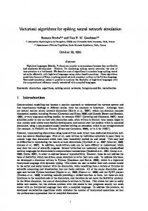
the spring, the elastic force F is directly proportional to the extension, or: (14) F = kx where k is the spring constant and x is distance of the displacement or extension of the spring. The elastic force F is the force necessary to restore the spring to its original length. In a mass and spring simulation, a damping coefficient is necessary as well to prevent the mass from oscillating indefinitely. Two robots, a and b, each of some finite mass, connected by a spring will have equal and opposite forces acting on each robot along the line that joins them. If there is a repulsive force - F acting on robot a, then there will be an attractive force F operating on robot b as follows: (15) Fa = k s (li − l 0 ) − k d x Fb = - Fa (16) (17) 0 < ks , kd < 1 where kd is the damping constant in Newton seconds per meter and ks is a spring constant in Newtons per meter. The first part of (15), ks(li-l0), is the spring force and the second part, k d x , is the damping or drag force that resists the motion and is proportional to the velocity. This force is a measure of how viscous the medium is that the spring is in. The control parameters are ks and kd. ks is a measure of how easy it is to extend or compress the spring. l0, the natural spring length, represents the desired spring length and is 5 meters for all simulations in this manuscript. Next, we demonstrate the effect of the control parameters on robot movement. Fig. 1 shows the initial configuration of 30 robots in an unbounded environment (no walls enclosing the robots). Fig. 2 is the simulation result after executing the EVSM algorithm with 30 robots using varying combinations of ks and kd with the self organizing force FSOF. The movement of the robots is in meters. A low ks and high kd will result in minimal robot movement. A high spring force parameter ks combined with a low damping coefficient kd will create maximum movement of the robots. As noted in [2], large robot movements due to a high ks and low kd, such as 0.9 and 0.1, respectively, may create instability in the mesh.
Fig. 1.Initial Robot Configuration with Varying Static ks, kd
performed, ∆W, in the spring, is proportional to the product of the damping force F3 in (5) and a distance through which the force is exerted, with both force and distance measured in the same direction [25]-[26]: t2 x2 t2 x2 dx (19) dt = k d ∫ x 2 dt ∆W = ∫ F3 dx = ∫ k d x dx = k d ∫ x t1 x1 t1 dt x1
Fig. 2. Effect of Control Parameters on Robot Movement
B. Mesh Stability This section discusses the states of the virtual spring mesh, mesh stability, energy dissipation, and switching. States of Virtual Spring Mesh. The virtual spring mesh can be in three different states: stable, quasi-stable, or unstable [4]. The mesh is stable, or has reached convergence, when the movement of each robot approaches zero, or the distance between robot neighbors is the natural spring length l0.
lim t →∞ pi (t ) − p j (t ) = l0
(18)
where pi(t) and pj(t) are the positions of robots i and j at time t, respectively. The mesh is quasi-stable when the robots wobble back and forth in a relatively stationary position. At this point the mesh itself is no longer moving but the robots appear to be in an oscillatory state and therefore wasting power. The mesh is unstable if not in a stable or quasi-stable state. Mesh Stability. The spring mesh achieves stability as the movement of all robots approaches zero, li→l0. However even with increased damping, kd↑, there will still be minute movement of the robots. Minute movements in an unchanging environment will cause a robot to move indefinitely in tight circles; i.e., a quasi-stable mesh. The virtual force vector F (F, θ) is driving robot movement and consists of both a magnitude F and a direction θ. Upper and lower bounds, vmax and vmin respectively, are placed on the robot movement. A robot movement ≥ vmax is set to vmax, and a movement ≤ vmin is set to zero. The mesh has stabilized when all robot movements are equal are zero. Too high a value for vmin will result in the robots stopping prior to achieving an optimal configuration. Too low a value for vmin will cause the robots to move in tight circles, wasting both time and energy. Energy Dissipation (Virtual). The virtual springs in EVSM are subject to a frictional or damping force, similar to a shock absorber in a car. The damping force is proportional to the velocity of the mass and acts in the direction opposite to the motion. Damping reduces the motion of the robot. The damping force in (1) and (5) is − k d xi where x is the velocity of the robot and k d is the damping coefficient. Energy is the ability to do work. Considering the damping force on a virtual spring, the dissipated energy, i.e. the work
Based on (5) and (19), work is proportional to damper force, and further damper force is proportional to speed: ∆W ∝ F3 and F3 ∝ x (20) hence ∆W ∝ x (21) Since the energy is defined as the ability to work, and work performed by robots is proportional to their speed, it can be concluded that the disipated energy of virtual springs is proportional to the speed of robots. . Switching. Energy in a virtual spring mesh system is affected by switching. Switching occurs when virtual springs are created or destroyed. When the mesh has stabilized, all switching has stopped. If a mesh is in a quasi-stable state (see previous paragraph on Mesh Stability), energy will continue to be dissipated because some robots continue to move in tight circles. As t→∞, the damping, F3 , and spring, F2 , forces will get in an equilibrium state (forces of same intensity but opposite direction), which will result in small (or no) robots’ speed, x , (speed meeting or dropping below threshold v min ). Finally, as robots stop moving, the disipating energy, proportional to the speed of robots, x , as shown in (21), will asymptotically aproach zero. Next, we review the theoretical aspects of mesh stability and time convergence. C. Theoretical Aspects of Mesh Stability The EVSM swarm algorithm is an example of a dynamic distributed control system. As time evolves the EVSM algorithm will cause the swarm to settle into a topology where each robot has a velocity that is approaching zero with interrobotic distances approaching the natural spring length. A global energy function for this system and Barbalat’s lemma [27]-[30] are used to prove convergence and stability in a spring mesh. References [31] and [32] have shown that the global energy function of (22) exists for a spring mesh. The terms within the left and right brackets of (22) represent potential energy (PE) and kinetic energy (KE), respectively. Both the PE and KE terms result in n x n matrices, where n is the number of robots in the swarm. Overdot represents differentiation with respect to time t, and XT denotes the transpose of matrix X. 1 1 Vσ (τ j ) = k s ( B. * D) + ( X T X ) 2 2
(22)
where •
σ (τ j ) determines who the immediate neighbors of a robot are by performing the acute angle test [1]. This function represents a switching of each robot’s virtual springs, or neighbors, over some time interval τj for the mesh.
•
•
D is an n x n displacement matrix where each cell is the square of the difference of the actual spring length minus the natural spring length. The mesh has stabilized if all elements of D are zero. When Dij is zero the robot distances to their neighbors are at the natural spring length. B is an adjacency virtual spring matrix for all robots where Bij = 1 represents a spring connection between robots i
and j X is a position vector is the acceleration vector for all robots X X is the velocity vector for all robots B.*D is an element-by-element multiple of these two matrices B and D are symmetric matrices, B=BT and D=DT. If a virtual spring exists in B between robots i and j, ri r j , then a virtual
• • • •
spring also exists between robots j and i, r j ri . Similarly, (lijl0)2 is equal to (lji-l0)2 in the displacement matrix D. An n x n matrix B is positive definite if y T By > 0 for all size-n vectors y≠0 [27], [33]. Both B and D contain only positive values and satisfy this criterion. An n x n matrix B is negative semidefinite if y T By ≤ 0, ∀y [27]. Equation (23) is the first derivative [32], [34] of the energy function (22) and represents the rate of energy dissipated by damping for all robots. V = − k ( X T X ) (23) σ (τ j )
d
The second derivative of the energy function from [31]-[32] is: = −2k ( X T X ) V (24) σ (τ j )
d
Barbalat’s lemma is a mathematical result concerning the asymptotic properties of functions and their derivatives. Barbalat’s lemma and the definiteness properties of (22)-(24) will be used to prove convergence and stability of the mesh over time. Barbalat’s lemma [27]-[30] states that for any function f(t), if f (t ) exists and is finite for all t, and 2) f (t ) is uniformly continuous (satisfied if f(t ) is finite) and negative semi-definite, (25) then lim f (t ) = 0
1)
t →∞
Since ks > 0 and B and D are positive definite, (22) is also positive definite and finite for all t, since X T X is a small term relative to B.*D. Robot velocities are limited to vmax and wireless sensing ranges limit the distance between robots thereby limiting X . The speed, X , cannot exceed vmax and therefore is bounded. Equation (23) is negative semi-definite for all values of X , so V can be either zero or negative (since X T X is always positive definite). V in (24) is bounded since
X is already shown to be bounded. Since V is bounded and
finite, V is uniformly continuous based on (25). Barbalat’s lemma can only be satisfied when V in (23) approaches 0 as t → ∞ as noted in (25). V can only approach zero when all elements in X are zero. Therefore all robot velocities eventually reach zero. D. Stability Surfaces for Mesh Simulations This section of the manuscript will introduce several 3D stability surfaces to describe and compare the behavior of the mesh for different simulations. The stability surface plots are for time steps to convergence, formation effectiveness, and potential energy of the mesh as shown in Fig. 3, 4, and 5, respectively, for 30 robots in an unbounded environment. Each simulation run is denoted by a large dot in these figures and is based on the initial configuration in Fig. 1. No boundary conditions are enforced so the behavior of the mesh can be observed in an unrestricted environment. The goal is to determine the ks and kd combinations that demonstrate the mesh is either in a stable or quasi-stable state. Time Steps to Convergence Stability Surface. Fig. 3 shows a time-step stability surface for 30 robots with both ks and kd varied from 0.1 to 0.9 in 0.1 increments with a vmin of 0.1 meter per second. The simulation is run in an unbounded environment; i.e., no wall boundaries. The number of time steps till the mesh achieves stability is plotted on the z axis. The simulation is stopped at 1000 time steps if the mesh has not achieved stability at that point. Stability is achieved when all of the forces acting on a robot in the spring mesh are zero.
∑
n
F=0
i =1
(26)
where F is the total force acting on a robot as defined in (6)
and n is the number of robots in the simulation. Fig. 3, and all subsequent 3D plots, depicts an interpolation of the surface at the data points represented by the large dots in the figure. The results of the plot are somewhat intuitive: • increasing ks while holding kd constant will, up to ks=~0.8, produce a stable mesh faster, and • very high values of ks result in a quasi stable mesh regardless of the damping factor. Formation Effectiveness Stability Surface. Fig. 4 shows the formation effectiveness stability surface as defined in (13) at the completion of each simulation for a specific ks and kd value. FE improves continuously with an increasing control parameter ks. The ideal FE stability surface would show high FE values for each simulation. Even small ks values result in less robot movement as noted in Fig. 2. And less movement requires more time to reach a desirable formation.
Fig. 3. Time Step Stability Surface Using Static Control Parameters, vmin = 0.1
Fig. 4. FE Stability Surface Using Static Control Parameters, vmin = 0.1
Potential Energy Stability Surface. The potential energy of robot i at an instant in time is the sum of the potentials to each of the robots neighbors connected via virtual springs [34]-[36]: 1 Ei = ∑ k s ( pi − p j − l 0 ) 2 (27) j ∈ Ni 2 The potential energy [31] of the entire mesh, where n is the number of robots in the mesh, is: 1 E p = ∑in=1 ∑ k s ( pi − p j − l0 ) 2 (28) j ∈ Ni 2 Fig. 5 shows the potential energy stability surface as defined by (28). The mesh approaches the desired formation as the sum of the potential energy of all the robots approaches zero [37]. As noted in (27) the potential energy of a robot is at a minimum when the distance to the robot’s neighbors approaches l0. The potential energy of a mesh is sometimes referred to as formation error [37] or deviation energy [38]. The ideal Ep stability surface would have Ep values at or close to zero for each simulation data point. Non-zero Ep values indicate the mesh has not achieved a perfect formation and may be in a quasi-stable state. Very small ks values produce very little movement of the robots resulting in EP greater than zero, meaning that the mesh still needs more time to reach a more optimal formation.
Fig. 5. EP Stability Surface Using Static Control Parameters, vmin = 0.1
IV. NOVEL ADAPTIVE CONTROL PARAMETER ALGORITHM TO IMPROVE SPRING MESH STABILITY This section addresses a novel approach for transitioning the mesh from a quasi-stable to a stable state by automatically and dynamically adapting the control parameters, ks and kd. Adaptive control parameters will be shown to achieve convergence and a near optimal formation in less time with fewer robot movements than with static control parameters. A high ks and low kd are desirable initially to enable the swarm to spread out as quickly as possible. After the mesh has spread out and the robot virtual springs approach their natural length, the goal is to enable the mesh to converge quickly by recognizing when a robot is in a quasi stable state. A robot then reduces their movement to vmin by executing the adaptive control parameter algorithm. When each robot has successfully executed this algorithm and their movements are equal to vmin, the mesh has reached convergence. Each robot automatically stops moving when their velocity reaches vmin. The adaptive control parameter algorithm works by automatically reducing ks and increasing kd as the movement of each robot approaches vmin. The desired formation of the swarm is achieved when (18) is satisfied for all robot neighbors. The virtual forces, or control laws, of (1), (10), and (11) governing the movement of robots are strongly impacted by both ks and kd. The movement of robot i with respect to a neighboring robot j using these control laws is based on ks, kd, and actual spring length between robot i and j, lij, and natural spring length l0 as noted in (29). lim (k s (lij − l0 ) uˆi − k d x ) ≤ vmin (29) k s ↓ , kd ↑
An increasing ks results in smaller changes to the virtual spring length, while a larger kd increases the damping applied to the virtual spring between robots i and j. When (29) reaches vmin for each robot, the mesh has achieved convergence. Robots make unnecessary movements and consume additional power when the mesh is in a quasi-stable state. An algorithmic approach for moving the mesh from a quasi-stable state to a stable state as quickly as possible will reduce both robot power consumption and time to achieve a near-optimal formation.
The terms and pseudo code to describe the adaptive control parameter algorithm are in Tables II and III, respectively. Parameter default values are noted in parenthesis. TABLE II ADAPTIVE CONTROL PARAMETER TERMS Term
Definition
Rk s
Rate of change of ks (0.0025) Rate of change of kd (0.0025)
Rkd
6. 7. 8. 9.
IF the average movement of the robot i is less than the threshold qs, then compare the robot damping control parameter kd to the upper bound for kd. The value of kd is decreased by Rkd since the damping parameter is less than the lower bound for kd. ENDIF ENDIF ks and kd are adjusted based on defined rates of change, Rk s
ks lower bound (0.1)
and Rk d , respectively. Empirical results have shown that rates
kd upper bound (0.9)
of change ≤ 0.25 with Lk s = 0.1 and Lk d = 0.9 produce stable
mi , s
Vector of last s movement distances for robot i
k si
Spring parameter for robot (0.8)
mesh configurations. The adaptive control parameter algorithm is executed when the robot is determined to be in a quasi stable state. A robot is in this state when two conditions are met: 1) FE between a robot and the virtual spring connections made to neighboring robots meets the formation effectiveness threshold, FET, and 2) the robot is moving in tight circles defined by a wobble radius, CR, from the centroid of the last n moves, where n is set to 10. FET and CR are set to 0.96 and 0.5 for all simulations in this manuscript unless otherwise noted.
Lk s U kd
Damping parameter for robot (0.1)
k di
qs CR FET
Quasi-stable threshold (0.0025) Wobble radius (0.5) Formation effectiveness threshold (0.96) TABLE III ADAPTIVE CONTROL PARAMETER ALGORITHM
Line #
Definition
1
Calculate mi ,s
2
IF mean(abs( mi ,s ))
3
IF
k si > Lks
k si = k si - k si * Rks
4 5
ENDIF
6
IF
7 8 9
< qs
k di < U k d
k di = k di + k di * Rkd ENDIF ENDIF
The adaptive control parameter algorithm requires separate ks and kd parameters for each robot. Next we describe each line of pseudo code in this algorithm outlined in Table III. 1. A vector of movement distances, mi,s, for robot i is calculated by determining the distance moved by the robot between time steps j and j+s for a window of s time steps. 2. IF the average of a vector of the absolute values of mi,s is less than the quasi-stable threshold qs, then make possible adjustments to the control parameters. The value of qs determines how quickly the control parameters will be adapted and bring the mesh to a stable state. If qs is set too high, the mesh will become stable before reaching an optimum state. If qs is too low, the robots will oscillate longer than necessary and use additional power. 3. IF the average movement of the robot i is less than the threshold qs, then compare the robot control parameter ks to the lower bound for ks. 4. The value of ks is decreased by Rks since the robot control 5.
parameter is greater than the lower bound for ks. ENDIF
V. SIMULATION TEST CASES A number of simulation test cases with and without obstacles in the environment will be exercised to validate our hypothesis that adaptive control parameters will enable mesh convergence; i.e., transition the mesh from a quasi-stable to a stable state. Boundary conditions for walls and offices/obstacles are observed by the EVSM algorithm. Simulation baseline test cases will first be developed using static control parameters with 30 and 120 robots in zero and five obstacle environments. Test cases using adaptive control parameters will then be compared to this baseline to contrast performance improvements and convergence. Time steps to converge, FE, and EP stability surface plots are used to compare the results of static versus adaptive control parameters. All simulations are run on a Dell computer, Intel Core 2 Quad CPU 2.33 GHz. MATLAB student version 7.8 was used to build all simulation models. Possible robots for implementing the EVSM algorithm include the iRobot SwarmBot (5in x 5in x 5in) or the Pioneer P3-DX (44cm x 38cm x 22cm). Single and multiple/varying simulation comparisons are run for areas with zero and five obstacles. The single simulation uses one ks and kd value, wheresas the varying simulation comparison uses a combination of ks and kd values. In previous work [1] we tried various static ks and kd combinations to determine the optimal values for these control parameters. A ks = 0.8 and kd = 0.1 have empirically been shown to result in a high FE and CE and therefore will be used in the following single control parameter simulations.
A. 70 x 50 Area with Zero Offices/Obstacles Single Control Parameter (ks, kd) Comparison. A building with a 70 x 50 meter space and no interior hard-walled offices/obstacles is shown in Fig. 6. This figure shows the final position of 30 robots after executing the EVSM algorithm with static control parameters. A high formation effectiveness of 95% is achieved after 1000 time steps. However the robots are still moving in tight circles with vmin set to 0.1 after 1000 time steps. The initial configuration was shown in Fig. 1 where the robots start out in the lower left hand corner of the area. As the simulation progresses and the mesh expands (Fig. 6), the edge robots reach the bottom and left wall boundaries, rather than the top and right wall boundaries, due to the robots close proximity to these walls. These edge robots anchor the mesh to the bottom and left wall boundaries because the application of the forces moves some of the robots to ~dmin distance of the walls and keeps them there. The remaining robots spread outward towards the top and right boundary walls until the virtual spring lengths approach l0.
Fig.7. CE and FE per Time Step with Static ks,kd
Fig. 8. Mesh with Adaptive ks,kd
Fig. 6. Mesh with Static ks,kd
Fig. 7 shows CE and FE plotted per time step. Both CE and FE peak relatively quickly at approximately 30 time steps and remain constant for the remainder of the simulation. The constant CE and FE achieved early in the simulation cycle demonstrate that the mesh deployment could have been terminated much earlier with no degradation of performance. Stopping the movement of the robots at the point FE plateaus, or the slope of the curve is zero, would transition the mesh from a quasi stable to a stable state and thus converge. The same simulation with 30 robots is now repeated but with adaptive spring parameters. Fig. 8 shows the mesh has transitioned from a quasi-stable to a stable state with an FE of 0.94 and a CE of 0.128 after only 32 time steps – a significant improvement over static control parameters. Rk s and Rk d are both 0.0025. The error E, 0.32 in Fig. 8, is the average virtual spring length deviation in meters from the natural spring length l0 of 5 meters. E is slightly larger for the adpative control parameters simulation than for the static control parameters, 0.32 versus 0.27. Adaptive control parameters provide a nearoptimal convergence of the mesh in term of E, and a highly optimal solution in terms of time to reach convergence. E may be reduced further by adjustments to FET, the formation effectiveness threshold, and CR, the wobble radius.
Varying Control Parameter (ks, kd) Comparison. Next, simulations are run for various ks and kd combinations using 30 robots to compare the performance of static versus adaptive control parameters. Fig. 9 and 10 show the time-step stability surfaces for 30 robots with static and adaptive spring parameters, respectively. Rk s and Rk d are both 0.0025 in Figs. 10 and 11. The adaptive control parameters enable convergence before 1000 time steps in all cases except for ks of 0.9 and kd of 0.1. These two values represent the extremes in the spring and damping parameters. A possible solution to achieving early convergence in this case is to increase the rates of change of both ks and kd, Rk s and Rk d , respectively.
Fig. 9. Time Step Stability Surface with Static ks, kd and vmin = 0.1
B. 70 x 50 Area with Five Offices/Obstacles Single Control Parameter (ks, kd) Comparison. The next sets of simulations are in a bounded environment with 5 obstacles. A mesh deployment takes longer in an environment with obstacles than in an obstacle free environment because more robot moves are required for the mesh to navigate around obstacles and cover the area. Also, obstacles that obstruct radio frequency signals and prevent robots from sensing their neighbors create discontinuities in the force laws due to the destruction of virtual springs. Fig. 10. Time Step Stability Surface with Adaptive ks, kd and vmin = 0.1
Fig. 11 shows FE per time step for several of the Fig. 10 simulations, where kd equals 0.1 and ks has values of 0.7, 0.5, 0.3, and 0.1. Note that in all cases the mesh has converged long before the 1000 time step time limit. The adaptive control parameter algorithm decreased ks and increased kd to transition the mesh from a quasi-stable to a stable state in 32 time steps, or less, for ks and kd combinations. The number of time steps required to reach convergence decreases as the value of ks is increased because of the larger movements of the robots over time with higher ks values. Additionally several other experiments were run to illustrate the improvement in algorithmic run time using adaptive springs. Table IV summarizes the results of 30 and 120 robot simulations in a zero office/obstacle environment with an initial ks=0.8 and initial kd=0.1 using both static and adaptive control parameters. The improvement in time steps with adaptive control parameters is significant with 30 robots. The 120 robot simulation with static control parameters is stopped at 1000 time steps without achieving convergence, while the adaptive control parameter simulation achieved convergence at 122 time steps. TABLE IV STATIC VS. ADAPTIVE CONTROL PARAMETERS, ZERO OFFICES Static Control Parameters Adaptive Control Parameters # Robots Time Steps Time Time Steps Time (minutes) (minutes) 30 74 0.24 29 0.10 120 NC NC 122 2.02 NC = No Convergence Achieved
Simulations of 120 robots with varying ks and kd combinations using static versus adaptive control parameters will now be compared in a five office/obstacle environment. The initial configuration of a building with 5 hard wall offices, or obstacles, and 120 robots is shown in Fig. 12. Fig. 13 shows the final position of 120 robots after running the EVSM algorithm with static control parameters ks and kd of 0.8 and 0.1, respectively, and vmin = 0.1. A formation effectiveness of 0.95 is achieved with the simulation stopped at 1000 time steps because of non convergence. The robots are still in a quasi-stable state, moving in tight circles, after 1000 time steps. Fig. 14 shows the final position of 120 robots after running EVSM using adaptive spring parameters. FE is the same as in the static spring case. The initial values of ks and kd are 0.8 and 0.1 whereas the final values are 0.38 and 0.2, respectively, due to the adaptive control parameter algorithm. However the mesh has transitioned from a quasi-stable to a stable state by the 405th time step. This is a significant improvement over the static control parameters of Fig. 13 where the mesh still remains in a quasi-stable state at time step 1000. Adaptive control parameters are clearly capable of transitioning the mesh from a quasi-stable state to a stable state. This results in reduced power consumption by the mobile robots and a significant reduction in time to reach a desireable degree of coverage.
Fig. 12.Five Office Initial Configuration with 120 Robots
Fig. 11. FE per Time Step with Adaptive Control Parameters and Varying ks
Fig. 13.Mesh with Static ks,kd in Five Office Environment
Fig. 14.Quasi-Stable to Stable Transition at Time Step 405 with Adaptive ks,kd
Varying Control Parameter (ks, kd) Comparison. Next, simulations are run for varying ks and kd combinations with 120 robots to compare the performance of static versus adaptive control parameters. Figs. 16 and 18, displayed in columnar format on the next page, are simulations with static control parameters. Whereas Figs. 15, 17, and 19, also displayed in columnar format on the next page, are simulations with adaptive control parameters. All simulations using static control parameters with 25 combinations of ks and kd resulted in no convergence after 1000 time steps. The simulations are stopped at 1000 time steps because of practical limits on battery power for the robots. Fig. 16 shows that formation improves with increasing ks as expected. Smaller values of ks mean smaller movements of a robot over time, requiring more time steps to reach convergence. 1000 time steps is insufficient for the mesh to reach convergence with small values of ks. Potential energy in Fig. 18 approaches, but will never reach, zero in this quasi-stable state. Potential energy will go to zero as a perfect formation is achieved in the mesh; i.e., li = l0 for all virtual springs. Note that with high values of ks, such as 0.9, and low values of kd, such as 0.1, FE decreases and EP rises, indicating some instability in the mesh with larger movements. Large movements may create instability in the mesh [2].
Fig. 15. Time Step Stability Surface with Adaptive ks, kd and vmin = 0.1
Fig. 16. FE Stability Surface with Static ks, kd, and vmin = 0.1
Fig. 17. FE Stability Surface with Adaptive ks, kd and vmin = 0.1
Fig. 18. EP Stability Surface with Static ks, kd and vmin = 0.1
Fig. 19. EP Stability Surface with Adaptive ks, kd and vmin = 0.1
Fig. 15 is the stability surface by time step for varying adaptive ks and kd, which is markedly different from the simulations with static control parameters where no convergence was reached for any control parameter combination. The swarm attains convergence for all ks values greater than or equal to 0.6. A possible solution to achieving convergence for ks values less than 0.6 is to increase the rates of change of both ks and kd, Rk s and Rk d , respectively, or decrease FET, the formation effectiveness threshold, and increase CR, the wobble radius. There are tradeoffs between convergence time, FE, and CE, and we are trying to optimize multiple objectives in a distributed manner. Fig. 17 shows the FE stability surface for varying adaptive ks and kd. The slope of the FE plot is more linear than in the static control parameter case which indicates that at lower values of ks, such as 0.3, FE is less optimal than for static control parameters. The stability surface for Ep in Fig. 19 also shows that the Ep is much higher at this ks value as well indicating that the virtual springs have not attained their natural length. FE and Ep would likely improve by adjusting the operating parameters previously noted for improving CE. Additionally several other experiments were run to illustrate the improvement in algorithmic run time using adaptive springs in a five office environment with 30 and 120 robots and ks and kd initially set to 0.8 and 0.1, respectively. The results are summarized in Table V. Both 30 and 120 robot simulations with static control parameters are stopped at 1000 time steps without achieving convergence. The adaptive control parameter simulation achieved convergence for the 30 and 120 robot simulations at 59 and 405 time steps, respectively. These results demonstrate that adaptive control parameters significantly improve the performance of the deployment of robots in mobile ad hoc network dispersion. TABLE V STATIC VS. ADAPTIVE CONTROL PARAMETERS, FIVE OFFICES Static Control Parameters Adaptive Control Parameters # Robots Time Steps Time Time Steps Time (minutes) (minutes) 30 NC NC 59 0.769 120 NC NC 405 24.69 NC = No Convergence Achieved
VI. CONCLUSION This manuscript presented a novel approach to dynamically adapting control parameters to achieve mesh configuration stability. The spring and damping control parameters, ks and kd, respectively, directly determine the movement of each robot in the mesh and govern the stability of the mesh. A mesh can be in either a stable, quasi-stable, or unstable state. A stable state exists when the robots in the mesh achieve convergence. A quasi-stable state exists when the robots move in tight circles in a small area without reaching convergence. Our hypothesis, which has been proven, was that automatically adapting the control parameters would transition the mesh from a quasi-stable to a stable state. The simulation results in this manuscript have demonstrated that adaptive control parameters are an effective approach for transitioning a mesh from a quasi-stable to a stable state and significantly reducing the convergence time. 120 robots reached convergence using adaptive control parameters more than twice as fast as with static control parameters in a multiple obstacle environment. VII. REFERENCES [1]
[2] [3] [4]
[5] [6] [7] [8] [9] [10] [11] [12]
[13]
[14]
K. Derr, M. Manic, “EVSM, the Algorithm for Distributed SelfOrganizing Mobile Ad Hoc Networks Exploration of Enclosed Areas”, IEEE Transactions on Industrial Electronics, Vol. 58, Issue 12, pp. 5424 – 5437, December 2011. B.Shucker, J. Bennett, “Virtual Spring Mesh Algorithms for Control of Distributed Robotic Macrosensors”, University of Colorado at Boulder, Technical Report CU-CS-996-05, May 2005. B.Shucker, J. Bennett, “Target Tracking with Distributed Robotic Macrosensors”, IEEE Military Communications Conference, October 1720, 2005, pp. 2617-2623. J. McLurkin, J. Smith, “Distributed Algorithms for Dispersion in Indoor Environments using a Swarm of Autonomous Mobile Robots”, Proceedings of the 6th international Symposium on Information processing in Sensor Networks, pp. 545-546, April 25-27, 2007. J. McLurkin,”Analysis and Implementation of Distributed Algorithms for Multi-Robot Systems”, PhD Dissertation, Massachusetts Institute of Technology, February 2008. W. Spears, D. Spears, “Distributed Physics-Based Control of Swarms of Vehicles”, Journal of Autonomous Robots, pp. 137-162, September 2004. M. Ma, Y. Yang, “Adaptive Triangular Deployment Algorithm for Unattended Mobile Sensor Networks”, IEEE Transactions on Computers, Vol. 56, No. 7, July 2007. O. Khatib, “Real-time obstacle avoidance for manipulators and mobile robots”, The International Journal of Robotics Research 5(1):90–98, 1986. R. Arkin, “Motor Schema-Based Mobile Robot Navigation”, The International Journal of Robotics Research 8, pp.92–112, 1989. T. Balch, M. Hybinette, “Social Potentials for Scalable Multi-Robot Formations”, IEEE International Conference on Robotics and Automation (ICRA-2000), San Francisco, 2000. A. Howard, M. Matari´c, “Cover Me! A Self-Deployment Algorithm for Mobile Sensor Networks”, Proceedings IEEE International Conference on Robotics and Automation ( ICRA ’02), pp. 80-91, May 2002. D. W. Gage. “Command control for many-robot systems”, AUVS-92, the Nineteenth Annual AUVS Technical Symposium, pages 22–24, Hunstville Alabama, USA, June 1992. Reprinted in Unmanned Systems Magazine, Fall 1992, Volume 10, Number 4, pp 28-34. S. Yoon, O. Soysal, M. Demirbas, C. Qiao, “Coordinated Locomotion and Monitoring using Autonomous Mobile Sensor Nodes”, IEEE Transactions on Parallel and Distributed Systems, Accepted for Publication in Future Issue, 2011. M. Schwager, J. Slotine, D. Rus, “Decentralized, Adaptive Control for Coverage with Networked Robots”, IEEE International Conference on Robotics and Automation, pp. 3289-3294, April 10-14, 2007.
[15] B.Shucker, J. Bennett, “Scalable Control of Distributed Robotic Macrosensors”, 7th International Symposium on Distributed Autonomous Robotic Systems, June 23-25, 2004. [16] N. He, D. Xu, “The Application of Particle Swarm Optimization to Passive and Hybrid Active Power Filter Design”, IEEE Transactions on Industrial Electronics, Vol. 56 No. 8, October 2009. [17] H. Chen, Y. Li, “Enhanced Particles with Pseudolikehoods for ThreeDimensional Tracking”, IEEE Transactions on Industrial Electronics, Vol. 56 No. 8, October 2009. [18] P. Persson, “Mesh Generation for Implicit Geometries”, PhD Dissertation, Massachusetts Institute of Technology, February 2005. [19] S. Owen, “Non-Simplical Unstructured Mesh Generation”, PhD Dissertation, Carnegie Mellon University, April 1999. [20] F. Sears, M. Zemansky, “University Physics, pp. 99-210, Addison Wesley, 1964. [21] F. Lewis, S. Jagannathan, A. Yesildirek, “Neural Network Control of Robot Manipulators and Nonlinear Systems”, Taylor and Francis Publishers, pp. 67-116, 1999. [22] J. Slotine, W. Li, “Applied Nonlinear Control”,Prentice Hall Publishes, pp. 123-126, 1999. [23] A. Dirafzoon, S.Salehizadeh, S. Emrani, M. Menhaj, A. Afshar, “Coverage Control for Mobile Sensing Robots in Unknown Environments Using Neural Network”, IEEE International Symposium on Intelligent Control, September 8-10, 2010. [24] M. Schwager, J. Slotiney, D. Rus, “Decentralized, Adaptive Control for Coverage with Networked Robots”, IEEE International Conference on Robotics and Automation, April 2007. [25] B. Shucker, T. Murphy, J. Bennett, “Switching Rules for Decentralized Control with Simple Control Laws”, American Control Conference, pp. 1485 – 1492, July 2007. [26] B. Shucker, T. Murphy, J. Bennett, “An Approach to Switching Beyond Nearest Neighbor Rules”, American Control Conference, pp. 5959 – 5965, June 2006. [27] T. Cormen, C. Leiserson, R. Rivest, C. Stein, “Introduction to Algorithms”, Prentice Hall, pp.725–769, August 2003. [28] B. Shucker, T. Murphy, J. Bennett, “Convergence-Preserving Switching for Topology-Dependent Decentralized Systems”, IEEE Transactions on Robotics, Vol. 24 No. 6, December 2008, pp. 1405 1415. [29] J. Reif, H. Wang, “Social Potential Fields: A Distributed Behavioral Control for Autonomous Robots”, Robotics and Autonomous Systems, Vol. 27, No. 3, pp. 171-194, May 1999. [30] M. Kass, “An Introduction to Physically Based Modeling: An Introduction to Continuum Dynamics for Computer Graphics”, Computer Graphics Tutorial, ACM SIGRAPH, 1997. [31] K. Hengster-Movric, S. Bogdan, I. Draga njac, “Bell-Shaped Potential Functions for Multi-Agent Formation Control in Cluttered Environment, 10th Mediterranean Conference on Control and Automation, Marrakech, Morocco, June 23-25, 2010. [32] H. Axelsson, A. Muhammad, M. Egerstedt, “Autonomous Formation Switching for Multiple, Mobile Robots”,I FAC Conference on Analysis and Design of Hybrid Systems, Sant-Malo, Brittany, France, June 2003 [33] K. Ogata, “System Dynamics”, Chapter 3 Mechanical Systems, Fourth Edition, Prentice Hall, August 2003. [34] B. Ranjbar-Sahraei, F. Shabaninia, A. Nemati, S. Stan, "A Novel Robust Decentralized Adaptive Fuzzy Control for Swarm Formation of Multiagent Systems", IEEE Transactions on Industrial Electronics, Vol. 59, No. 8, August 2012. [35] G. Lee, N. Chong, "Low-Cost Dual Rotating Infrared Sensor for Mobile Robot Swarm Applications", IEEE Transactions on Industrial Informatics, Vol. 7, No. 2, May 2011. [36] P. Vicaire, E. Hoque, Z. Xie, J. Stankovic, "Bundle: A Group-Based Programming Abstraction for Cyber-Physical Systems", IEEE Transactions on Industrial Informatics, Vol. 8, No. 2, May 2012. [37] C. Tsai, H. Huang, C. Chan,"Parallel Elite Genetic Algorithm and Its Application to Global Path Planning for Autonomous Robot Navigation", IEEE Transactions On Industrial Electronics, Vol. 58, No. 10, October 2011. [38] G. Zhao, K. Xuan, W. Rahayu, D. Taniar, M. Safar, M. Gavrilova, B. Srinivasan, "Voronoi-Based Continuous k Nearest Neighbor Search in Mobile Navigation", IEEE Transactions on Industrial Electronics, Vol. 58, No. 6, June 2011.
Kurt Derr (M’04): Kurt Derr, IEEE Member, has a B.S. in Electrical Engineering from Florida Institute of Technology and an M.S. in Computer Science from the University of Idaho. He is currently pursuing a PhD in Computer Science from the University of Idaho. Kurt has worked as a Computer Scientist at the Idaho National Laboratory since 1986 and began teaching courses as Affiliate Faculty at the University of Idaho in 1987. He received an R&D 100 award in 2009 for RFinity, Mobile Open-Encryption Platform and has coauthored 4 patents. Kurt has also written a book on object-oriented technology, Applying OMT, published in 1995. He has several recent published papers at IEEE conferences on computational intelligence in wireless networking environments. Milos Manic, PhD (S'95-M'05-SM'06): Dr. Milos Manic, IEEE Senior Member, has been leading Computer Science Program at Idaho Falls and is a Director of Modern Heuristics Group. He received his Ph.D. degree in Computer Science from University of Idaho, Computer Science Dept. He received his M.S. and Dipl.Ing. in Electrical Engineering and Computer Science from the University of Nis, Faculty of Electronic Engineering, Serbia. He has over 20 years of academic and industrial experience, including an appointment at the ECE Dept. and Neuroscience program at University of Idaho. As university collaborator or principal investigator he lead number of research grants with the Idaho National Laboratory, NSF, EPSCoR, Dept. of Air Force, and Hewlett-Packard, in the area of data mining and computational intelligence applications in process control, network security and infrastructure protection. Dr. Manic an Administrative Committee Member for the IEEE Industrial Electronics Society and member of several technical committees and boards of this Society. Dr. Manic has published over hundred refereed articles in international journals, books, and conferences.