Dec 2, 2016 - Table 1 lists the values for central tendency, dispersion, kurtosis ... that the Shapiro-Wilk and Shapiro-Francia tests offer better performance.2,9- ...
EDITORIAL
Assessing normality of data in clinical and experimental trials Avaliação da normalidade dos dados em estudos clínicos e experimentais Hélio Amante Miot1
*
When continuous data are used to represent natural events they can take a variety of different frequency distributions, one of which is a bell-shaped distribution that is known as the normal or Gaussian curve (Figure 1). Normal curves have properties that make them special from a statistical perspective, particularly their symmetry, their unique mode (which is the same as both the mean and the median), and the fact that they can be represented and quantified from the values of the mean and the standard deviation.1 The main statistical tests used for analysis of clinical and experimental data are based on theoretical models that assume a normal distribution, such as Student’s t test, ANOVA, Pearson’s coefficient, linear regression (residuals), and discriminant analysis.2 For this reason, testing data distributions for normality is an essential element of adequately describing samples and their inferential analysis.3 Sample size calculations are also influenced by the underlying data distribution.4 Many biomedical data have non-normal distributions, especially those representing events with great variability, with a standard deviation greater than half of the mean value (Figure 2); which contraindicates the use of statistical techniques appropriate for normal samples, which would risk introducing bias to parameters and
to the inferences of tests.2,5 Even increasing the sample size cannot correct the estimation errors caused by using analytical techniques that are not suited to the data distribution. The first step in evaluating the normality of a dataset should be to examine its histogram to identify major asymmetries, discontinuity of data, and multimodal peaks. It is also important to stress that when analyzing subsets or conducting multiple comparisons, all of the categories or subsamples being analyzed must be tested for normality, and not just the overall sample.2,3 Figure 1 shows a histogram plotted from data that are approximated to the normal distribution, whereas Figure 2 shows an asymmetrical histogram, that are approximated to the gamma distribution. Assuming that the histogram does not reveal elements that are not consistent with the normal distribution, it is then recommended that estimators of symmetry and kurtosis should be calculated. These represent elements related to the shape of the histogram, dislocation to the left/right (symmetry) or peaked/flattened shapes (kurtosis), and both these measures approach zero when data are normal. Since these estimators are affected by sample size and outliers, it is prudent to calculate the ratio of their values to the standard error of their
Figure 1. Patients (n = 89) with venous ulcers treated at the Dermatology Service, Faculdade de Medicina de Botucatu, Universidade Estadual Paulista (UNESP), SP, Brazil: histogram and Q-Q plot for age in years. Universidade Estadual Paulista – UNESP, Faculdade de Medicina de Botucatu, Departamento de Dermatologia e Radioterapia, Botucatu, SP, Brazil. Financial support: None. Conflicts of interest: No conflicts of interest declared concerning the publication of this article. Submitted: December 02, 2016. Accepted: December 14, 2016. 1
88
J Vasc Bras. 2017 Apr.-Jun.; 16(2):88-91
http://dx.doi.org/10.1590/1677-5449.041117
Hélio Amante Miot
estimates. In general, the result of dividing the value of the coefficient by its standard error should fall in the range -1.96 to +1.96 for normal distributions.6 Table 1 lists the values for central tendency, dispersion, kurtosis, and symmetry for the distributions illustrated in Figures 1 and 2. It can be observed that the values for symmetry and for kurtosis for the data on area of ulcers are both far from zero and dividing them by their standard errors produces values greater than 1.96: 10.5 and 12.0. Quantile-quantile plots (Q-Q plots) are graphical illustrations of the proportions of the data from the original sample compared against the quantiles expected for a normal distribution (Figures 1 and 2). Ideally, the Q-Q plot should follow a diagonal line if the data distribution is close to normal. The same analysis can be conducted using P-P plots, in which the distribution of the observed data is compared with the cumulative percentile expected from a normal distribution. There is a tolerance for minor deviations that occur at the extremes, as illustrated by the error lines plotted in Figure 1. In general, analyses of normality based on Q-Q plots are more reliable for large-scale samples (> 5,000 units), when tests of
normality can greatly inflate type II error (reducing sensitivity).7,8 There are dozens of statistical tests for verifying the fit of data to a normal distribution, based on different assumptions and using different algorithms. All of them test the null hypothesis (H0) that the data are normal, and so they return p-value > 0.05 if the result shows that data do fit the parameters for normality. Several simulations have demonstrated that the Shapiro-Wilk and Shapiro-Francia tests offer better performance.2,9-14 The efficacy of normality tests suffers influence from sample size. With small samples (from 4 to 30 units), type I error is inflated and the Shapiro-Wilk and Shapiro-Francia tests are preferable (for better specificity). As sample sizes increase, especially over 500 units, all of the tests offer better performance; however, it is prudent to adopt a significance level of p < 0.01, because of the inflation of type II error caused by larger samples (reducing sensitivity).2,11,14 The D´Agostino-Pearson test was developed to deal with larger samples (n > 100), in which case it offers similar performance to the Shapiro-Wilk test. The Jarque-Bera test offers good performance for
Figure 2. Venous ulcers (n = 125) in patients treated at the Dermatology Service, Faculdade de Medicina de Botucatu, Universidade Estadual Paulista (UNESP), SP, Brazil: histogram and Q-Q plot for areas in cm2. Table 1. Estimators of central tendency, dispersion, and certain tests of normality related to data for patient age and area of 125 venous ulcers in 89 patients treated at the Dermatology Service, Faculdade de Medicina de Botucatu, Universidade Estadual Paulista (UNESP), SP, Brazil. Age (years) Mean (standard deviation) Median (p25-p75) Kurtosis (standard error) Symmetry (standard error) D´Agostino-Pearson test (p-value) Lilliefors test (p-value) Shapiro-Wilk test (p-value)
62.1 (11.6) 60.6 (53.0-71.8) -0.50 (0.51) -0.14 (0.26) 1.41 (0.50) 0.05 (0.66) 0.99 (0.71)
Area of ulcer (cm2) 39.3 (62.9) 11.4 (4.0-38.4) 5.14 (0.43) 2.30 (0.22) 55.52 (