Assessing Temporal Emotion Dynamics Using Networks Laura F. Bringmann, Madeline L. Pe, Nathalie Vissers, Eva Ceulemans, Denny Borsboom, Wolf Vanpaemel, Francis Tuerlinckx, Peter Kuppens KU Leuven
Introduction Experience sampling methods (ESM; Csikszentmihalyi & Larson, 2014; Trull & Ebner-Priemer, 2013) and ecological momentary assessment (EMA; Shiffman & Stone, 1998; Stone & Shiffman, 1994) are being increasingly used to study dynamic psychological processes such as mood (aan het Rot, Hogenelst, & Schoevers, 2012; Hamaker, Ceulemans, Grasman, & Tuerlinckx, 2015; Jahng, Wood, & Trull, 2008; Wichers, Wigman, & Myin-Germeys, in press). A particularly relevant aspect thereof is their temporal dynamics (Nesselroade, 2004).1 When studying temporal dynamics, the focus is not on detecting a gross underlying trend, as is often the case in developmental research, but rather on the intricate temporal dependence of and between variables, or how variables within an individual influence each other or themselves over time (Brandt & Williams, 2007; Molenaar, 1985; Walls & Schafer, 2006). Often the models used to study temporal dynamics are multivariate in nature, and both the influence that a variable has on itself (e.g., how self-predictive is sad mood) as well as its effects on other variables (e.g., how does sad mood augment or blunt subsequent anger emotions) are analyzed (Koval, Pe, Meers, & Kuppens, 2013; Kuppens, Stouten, & Mesquita, 2009; Kuppens, Allen, & Sheeber, 2010; Pe & Kuppens, 2012; Suls, Green, & Hillis, 1998). One increasingly popular approach to study, visualize, and analyze multivariate dynamics is network analysis (Borsboom & Cramer, 2013; Bringmann, Vissers, et al., 2013; Bringmann, Lemmens, 1
Address for correspondence: Department Quantitative Psychology and Individual Differences; University of Leuven;
Tiensestraat 102 - box 3713; 3000 Leuven; Belgium; tel.+32163 26052; email:
[email protected]. The research leading to the results reported in this paper was sponsored in part by Belgian Federal Science Policy within the framework of the Interuniversity Attraction Poles program (IAP/P7/06), as well as by grant GOA/15/003 from the KU Leuven, and grant G.0806.13 from the Fund of Scientific Research Flanders.
Huibers, Borsboom, & Tuerlinckx, 2015; Fried, Nesse, Zivin, Guille, & Sen, 2014; McNally et al., 2015; Ruzzano, Borsboom, & Geurts, 2015; Wichers, 2014). This network perspective leads to a new way of thinking about the nature of psychological constructs, phenomena or processes by offering new tools for studying dynamical processes in psychology. In the network approach, psychological constructs, processes or phenomena are represented as complex systems of interacting components (Barab´asi, 2011; Costantini et al., 2015; Cramer, Borsboom, Aggen, & Kendler, 2012). For instance, emotional well-being can be considered to consist of a number of dynamically interacting components, such as behavioral, physiological, and experiential emotion components. Likewise, mental disorders can be viewed as a result of the mutual interplay of symptoms of the disorder. These components interact with each other across time, making up the internal dynamics and by that, the very nature of the phenomenon under study. It is these dynamics that are studied in a network approach (Borsboom, Cramer, Schmittmann, Epskamp, & Waldorp, 2011; Cramer, Waldorp, van der Maas, & Borsboom, 2010; Schmittmann et al., 2013). In this paper, we will illustrate the network approach using an empirical example focusing on the relation between the daily fluctuations of emotions and neuroticism.
The network approach A network consists of nodes (i.e., the components of the phenomenon, construct or process) and edges (or links) connecting the nodes (Barrat, Barthelemy, Pastor-Satorras, & Vespignani, 2004). In our approach, the links have a certain strength that indicates the strength of the (positive or negative) relationship between the nodes (Opsahl, Agneessens, & Skvoretz, 2010). The nodes and edges can be easily visualized graphically (see for example Figure 1). Networks can be constructed based on different kinds of data such as cross-sectional or longitudinal data and using different kinds of models for inferring the edges. Depending on the data and model used to infer the network, the edges connecting the nodes have a specific meaning. In this article, we focus on longitudinal data and on the vector autoregressive (VAR) model (Brandt & Williams, 2007). A VAR-based network allows studying the dynamics among the components that constitute a certain construct, phenomenon or process across time. For example, in the network of Figure 1, the edges on the nodes are the self-loops, or the effect the emotion has on itself from one time point to the next, and the edges between the emotions are the cross-regressive effects, or the effect a variable has on other variables from one time point to the next, controlling for the other variables. In addition, several features of the network can be derived that can shed light on central properties 2
Angry
Sad
Happy
Figure 1.
A hypothetical example of an emotion network. The three nodes are the three emotions: Happy,
Angry and Sad. The red arrows are the negative (i.e., inhibitory) edges and the green arrows the positive (i.e., excitatory) edges. The thickness of the arrows represents the strength of the edges. For example, the edges on the nodes (the self-loops) are the strongest links in the network.
3
of the dynamical interplay between the components or nodes. Such features can involve the overall network or specific parts of the network. One interesting characteristic of the overall network is its density, which indicates how strongly the network is interconnected. The denser a network is, the more strongly the variables interact (Newman, 2010). Another, more specific, feature of the network is node centrality. Centrality refers to the importance or how focal one specific variable or node is in the network (Freeman, 1978).
Empirical example
We will illustrate how networks can be inferred using a multilevel extension of the VAR model (Bringmann, Vissers, et al., 2013), and how they can be used to gather new insights on temporal emotion dynamics. In particular, we will focus on the relation between emotion dynamics and neuroticism in healthy subjects, using two previously collected ESM datasets. Neuroticism is one of the main dimensions reflecting individual differences in personality, and is particularly relevant for emotional experience. Specifically, it reflects a tendency to experience negative emotions, and is considered to constitute a broad risk factor for mood disorder and psychopathology (Barlow, Sauer-Zavala, Carl, Bullis, & Ellard, 2014). In this application, we will first look at the general patterns of edges connecting the emotion variables, which are referred to as the population networks. Second, we will assess features of the network structure by studying the density of the individual emotion networks and their relation to neuroticism. In a third step, we will study whether several centrality measures of the individual networks (strength, closeness and betweenness) and the self-loops are related to neuroticism. To our knowledge, this is the first time that both the full temporal emotion network and its parts are studied and related to neuroticism, giving a more complete picture of moment-to-moment dynamics in emotion as a function of the trait of neuroticism. The method used here will be described in detail. Moreover, Matlab and R code to replicate the main results of the first dataset will be given, so that other researchers can apply the network method to their own data (see Appendices).2
2
To use this code please read first the R file.
4
Method Dataset 1 Parts of dataset 1 have been published elsewhere (Bringmann, Vissers, et al., 2013; Koval, Kuppens, Allen, & Sheeber, 2012; Pe, Koval, & Kuppens, 2013; Pe, Raes, et al., 2013). 95 undergraduate students from the University of Leuven in Belgium (age: M = 19 years, SD = 1; 62% female) participated in an experience sampling method (ESM) study. Over the course of seven days, participants carried a palmtop computer on which they had to fill out questions about mood and social context in their daily lives 10 times a day. Participants were beeped to fill out the ESM questionnaires at random times within 90-minute windows. They had to rate, among other things, their current feelings of negative and positive emotions on a continuous slider scale, ranging from 1 (not at all, e.g., angry) to 100 (very, e.g., angry). On average, participants responded to 91% of the beeps (SD = 7 %). In order to avoid selection bias, we analyzed all six emotion variables measured in this study (positive affect: relaxed and happy; negative affect: dysphoric, anxious, sad and angry), which were selected to capture all quadrants of the affective circumplex defined by the dimensions of valence and arousal (see e.g., Russell, 2003). Furthermore, neuroticism was assessed with the Dutch version of the Ten Item Personality Inventory (Gosling, Rentfrow, & Swann, 2003; Hofmans, Kuppens, & Allik, 2008), resulting in a score ranging from 1 to 7 (M = 3.4; SD = 1.5). Participants were selected from a large pool of participants to ensure a wide range of depression scores. Therefore, the participants in this dataset have a wider range of neuroticism scores than the participants in dataset 2. Dataset 2 Parts of this dataset have been published elsewhere (Kuppens, Champagne, & Tuerlinckx, 2012; Kuppens, Oravecz, & Tuerlinckx, 2010; Pe & Kuppens, 2012). In this study, the participants consisted of 79 undergraduate students from the University of Leuven in Belgium (age: M = 24, SD = 8; 63 % female). A similar ESM procedure as in the first dataset was used. Participants were beeped to fill out the ESM questionnaires 10 times a day, again on a scale ranging from 0 to 100, but for a longer time period, namely 14 consecutive days. We extracted all emotion variables, which were 10 in this case (positive affect: relaxed, happy, satisfied, excited; negative affect: dysphoric, anxious, irritated, sad, stressed and angry), again selected to cover all quadrants of the affective space. Participants responded on average to 82% of the programmed beeps (SD = 10). Neuroticism was assessed with the 12-item scale of the Dutch version of the NEO Five-Factor Inventory (Hoekstra, Ormel, & De Fruyt, 1996), 5
which resulted in a score ranging from 1 to 5 (M = 3.0, SD = 0.7). Estimating the networks To assess temporal emotion dynamics and their relation to neuroticism, an emotion network was created for each individual. The edges or links of the individual networks were obtained using a multilevel VAR model (Bringmann, Vissers, et al., 2013; Bringmann et al., 2015). The standard VAR model (Brandt & Williams, 2007) estimates the extent to which a current emotion (time point t) can be predicted from all other emotions at a previous moment (time point t − 1), corresponding to the network edges. Each emotion is regressed on its lagged values (autoregressive effect) and the lagged values of each of the other emotions (cross-lagged effects). In the present context, time t − 1 and time t refer to two consecutive beeps within the same day (overnight lags were removed). It is assumed that the data are stationary, implying that the mean and the moment-to-moment interactions of the emotion processes stay stable over time (Chatfield, 2003; Hamaker & Dolan, 2009). As we study multiple individuals, we implement the VAR model within a multilevel modeling framework, to allow for random, personspecific auto- and crossregressive effects, and so that we can model the temporal emotion dynamics not only within an individual, but also at group level, estimating both average or population (fixed) and individual (random) effects. Univariate multilevel VAR analyses are conducted for each emotion separately using restricted maximum likelihood estimation. This results in 6 univariate regression equations for the first dataset and 10 univariate regression equations for the second dataset. Taking the first dataset with 6 emotions as an example, we get the following equation for each emotion j (i.e., relaxed, happy, dysphoric, anxious, sad and angry, or j = 1, . . . , 6, respectively): Yptj = γ0pj + γ1pj · relaxedp,t−1 + γ2pj · happyp,t−1 + γ3pj · dysphoricp,t−1
(1)
+ γ4pj · anxiousp,t−1 + γ5pj · sadp,t−1 + γ6pj · angryp,t−1 + εptj . Thus, for dataset 1, Yptj represents the value for the j-th emotion for person p (p = 1, 2, . . . , 95) at beep t (t = 2, . . . , 10). The regression coefficients (i.e., the intercept and the regression weights) of this equation 1 are decomposed as follows: γkpj = βkj + bkpj ,
(2)
where the slopes βkj (k > 0, since k = 0 codes for the intercept) represent the fixed effects (the edges in the network), or the extent to which the emotions at time t − 1 can predict the emotion j 6
at time t over all individuals. The person-specific deviation (random effect) from the average effect is captured in the component bkpj . The random effects are assumed to come from a multivariate normal distribution, estimating an unstructured covariance matrix of the random effects. Using the empirical Bayes estimates of the random effects, emotion networks for each individual are constructed. Specifically, for each edge in the network, the individual random effect is added to the fixed effect for each emotion variable. For instance, the edge from emotion k to emotion j has a value of γkpj = βkj + bkpj in the individual network of person p. To reduce the likelihood of errors in the analyses, all multilevel analyses were run in Matlab (Mathworks, Inc.) as well as in Mplus (Muth´en & Muth´en, 2012) and by different researchers. Visualization and computation of the measures of centrality relied on the qgraph R package (Epskamp, Cramer, Waldorp, Schmittmann, & Borsboom, 2012). Regarding the analysis, there are three important additional aspects to mention here. First, as we estimate multivariate networks with both autoregressive and cross-lagged effect, all predictors were person-mean centered (centered around each individual’s mean score) before the analysis (Hamaker & Grasman, 2014). Note that this might lead to a slight underestimation of the autoregressive effects. Second, to control for differences in variability between individuals, i.e. to make sure that associations between neuroticism and network characteristics were not driven by differences in emotion variance, we conducted analyses involving both non-standardized and standardized coefficients.3 Within-person standardization of the coefficients was done as described in (Schuurman, Ferrer, de Boer-Sonnenschein, & Hamaker, in press).4 Third, note that the edges only represent the unique direct effects of the variables and not the shared effects (just as in standard multiple regression; Bulteel, Tuerlinckx, Brose, & Ceulemans, in press). This means that a part of the explained variance cannot be taken into account and thus an edge might be less strong or stronger if this shared variance was taken into account.
Network analyses The population networks Before we focus on individual networks and their relationship to neuroticism, we will first look at the average networks. These population networks show the general patterns of connections between the emotion variables. The edges in the population networks represent the slopes βkj (k > 0; i.e., the fixed 3
One exception is the analyses using self-loops. In order to standardize the edges of the network, the standard
deviations of the predictor and outcome variables are used. Since a self-loop has the same predictor as outcome variable the standardized and unstandardized edges are equal. 4 Note that there are different ways to standardize that lead to slightly different results.
7
effects). The population networks are presented in Figure 2, made with the R-package qgraph (Epskamp et al., 2012). Density For each individual network, the density was computed of 1) the overall network (all emotions), 2) the negative emotions only and 3) positive emotions only. This was done by averaging over the absolute values of the slopes or edges in the network of the emotions of interest. We used the absolute values so that negative and positive edge values do not cancel each other out. Further, to illustrate the relation between density and neuroticism, we created three neuroticism groups (i.e., low, medium and high neuroticism) by ranking the neuroticism scores. In a next step, we constructed networks for the low and high neuroticism group separately (eventually resulting in two networks for overall, negative and positive emotion density for both datasets). If we focus on the overall network for simplicity of explanation, then the arrows indicate the edge strengths of the temporal connections between emotions. The average absolute value of the edge strength and the corresponding standard deviation (SD) is calculated across all participants and pairs of variables. Next, edges get classified: 1SD below the mean (weak connection strength, dotted arrows), between 1SD below and above the mean (moderate connection strength, dashed arrows) and 1SD above the mean (strong connection strength, solid arrows). Centrality We calculated the most common centrality measures degree (or in case of a weighted network the term strength is used), closeness and betweenness. Each centrality measure defines centrality of a node (variable) in the network in a different way (Freeman, 1978; Newman, 2010). To explain these concepts, it is instructive to think metaphorically that the nodes transmit information across time to each other. As the network used here is a directed network, we can study both the out-strength centrality and the in-strength centrality. Out-strength indicates the (summed) strength of the outgoing edges or how much information a node sends away to the other nodes, and thus a node with a high out-strength centrality tends to excite or inhibit many other nodes in the network. In-strength indicates the strength of the incoming edges, or how much information a node receives from the other nodes, and thus its susceptibility to being excited or inhibited by other nodes in the network.5 Both out- and in strength take only into account the edges to which a node is directly connected. 5
We thank an anonymous reviewer for suggesting this interpretation.
8
A node high in closeness centrality is at a relatively short distance from the other nodes in the network, and is thus likely to be influenced quickly by them. Closeness thus represents how fast an emotion can be reached from the other nodes in the network. Distances between nodes are calculated based on edge strength, taking into account direct and indirect edges connecting the node to other nodes (See for more information: Borgatti, 2005; Costantini et al., 2015; Opsahl et al., 2010). Betweenness centrality is a measure of how many times a node appears on the shortest paths between other nodes in the network. Thus, a node with a high betweenness centrality is a node through which the information in the network has to pass often and can be seen as an important node in funneling the information flow in the network. This measure also takes into account direct and indirect edges connecting the node to other nodes. Note that all the centrality measures are based on the absolute values of the edges.
The relation between the network characteristics and neuroticism Neuroticism scores of all individuals were correlated with density of the individual networks (calculated on the overall, negative and positive networks) and centrality measures (out-strength, in-strength, closeness and betweenness) using Pearson’s product moment correlations. Since the centrality measures are concerned with the influences between variables or nodes (cross-regressive effects) in the network, self-loops or autoregressive effects (in the emotion literature also known as emotional inertia; Suls et al., 1998) are ignored in these focal network measures. Therefore, the correlation between the self-loops and neuroticism was calculated separately for each emotion.
Results The networks in Figure 2 represent the average patterns between the emotions. Only edges that were significant (i.e., a p − value of less than 0.05) are shown, which is purely for visualization purposes. The figures show that emotions can either augment or blunt each other (Pe & Kuppens, 2012). Augmenting refers to the increase of the experience of other emotions. For example, there exist clusters of negative and positive emotions. Within these clusters, emotions of the same valence tend to in general augment each other. In contrast, emotions of different valence (for example, sad and happy) seem to blunt or decrease each other. Furthermore, the self-loops in the networks are among the strongest edges. For example, in general when a person feels sad, (s)he is not only less likely to feel happy at the next 9
moment, but also likely to still experience sadness at the next moment.6 These results correspond with the theoretical expectations and empirical findings based on the nomothetic relations in an emotion circumplex, namely that emotions of the same valence are more likely to be correlated with each other than with emotions of different valence (Vansteelandt, Van Mechelen, & Nezlek, 2005). Dataset 1
Dataset 2
Angry
Angry Excited
Stressed
Happy
Anxious
Sad
Irritated
Happy
Anxious
Satisfied
Relaxed
Sad Dysphoric
Relaxed
Dysphoric
Figure 2. This figure shows the population network of the dataset 1 (left panel) and the dataset 2 (right panel). Solid green edges correspond to positive and dashed red edges to negative connections. Only edges that surpass the significance threshold are shown (i.e., for which the p-value of the t-statistic is smaller than 0.05). The emotions in the networks are organized so that they align with the emotion circumplex from which they were selected.
The results in Table 1 show a consistent and strong positive relation between neuroticism and overall emotion density as well as negative emotion density. This pattern is not only consistent across datasets, but also when controlling for variability (i.e., after standardization), indicating that individuals high in neuroticism also have a significantly denser overall network and negative emotion network than individuals low in neuroticism. The results for the positive emotions emotion network were less consistent. The relation between the positive emotion network and neuroticism was only significant in the second dataset and was less strong than the relationship between neuroticism and the overall and negative emotion networks. Figures 3 and 4, focusing on the high and low ends of neuroticism, also 6
Note that the number of possible edges is proportional to the number of nodes and thus the network for dataset 2 is
not necessarily more strongly connected than the network for dataset 1.
10
features this pattern: The difference between emotion density in individuals with a high and low score in neuroticism is more pronounced for the overall emotion density and negative emotion density than for positive emotion density.
Table 1: Density and its relation to neuroticism
Non-standardized Data 1 Emotion N etwork
r
p
Standardized
Data 2 r
p
Data 1 r
p
Data 2 r
p
Overall
.49