An argumentation network has the form (AR, Attack), ... tive factors in Support and Attack networks is twofold. ... (b) The situation in Figure 2 is a complete loop.
Temporal Dynamics of Support and Attack Networks: From Argumentation to Zoology Initial Results Howard Barringer1, Dov Gabbay2 , and John Woods3 1
School of Computer Science, The University of Manchester, Oxford Rd, Manchester M13 9PL, UK 2 Department of Computer Science, King’s College London, Strand, London WC2R 2LS, UK 3 Department of Philosophy, University of British Columbia, 1866 Main Mall E370, Vancouver BC Canada V6T 1Z1
1
Introduction
This is the first of a new series of papers on the temporal dynamics of Support and Attack networks. These are graphs with a basic situation described in Figure 5 below. We have nodes a1 , . . . , an connected by arrows to a node b. The nodes have some values attached to them and these values are transmitted by the arrows, and revise the value at b. This series of papers studies the temporal dynamics of such networks. The topic, in this generality, has emerged from our previous research into argumentation frameworks (Gabbay and Woods [14, 13, 10, 12] and Woods [21]). Our starting point is therefore a generalisation of abstract argumentation networks. Abstract argumentation frameworks were put forward by Dung [5] following the realisation that in real life every argument has a counter argument and no argument is conclusive. An argumentation network has the form (AR, Attack), where AR is a set of arguments and Attack ⊆ AR2 is an irreflexive binary relation on AR, indicating which argument attacks which arguments. We should emphasise that our approach here is dialectical rather than normative. When we say that every argument has a counterargument it is not our view that every argument deserves a counter, but rather than every argument, whatever its merits, lies open to a counter, whatever its merits. We say that no argument is conclusive, we intend that every argument is susceptible to challenge, again notwithstanding its presumed merits. And when we say (just below) that any argument that attacks an argument is a refutation of it, we intend only that the attacking argument is presented as a refutation and that the attacked argument is, on that argument, put under challenge. Our purpose in emphasising descriptive factors in Support and Attack networks is twofold. We have reservations about the speed with which some argumentation theorists rush to normative judgement; and, in any event, we take description to have an expository priority over normative considerations in theoretical accounts of argumentative practice. D. Hutter, W. Stephan (Eds.): Mechanizing Mathematical Reasoning, LNAI 2605, pp. 59–98, 2005. c Springer-Verlag Berlin Heidelberg 2005 �
60
Howard Barringer, Dov Gabbay, and John Woods
Example 1. Figures 1 to 3 are three examples of such networks.
a
c
b Fig. 1.
c
a
b Fig. 2.
a
b
c
d Fig. 3.
(a) The situation in Figure 1 is straightforward. a is not attacked by anything, so it is in (or active) as an argument. Since it attacks b, b is out (or is a refuted argument) and so c is in. So the net result of Figure 1 can be written as {+a, −b, +c}. (b) The situation in Figure 2 is a complete loop. No argument can definitely be said to be in or out. We write this as {?a, ?b, ?c}. (c) The situation in Figure 3 is more interesting. Here a and b attack each other; so we have ?a, ?b. Because of that, we can also put it that ?c and ?d. However we can observe that both a and b attack c; so no matter which of a or b are in (i.e. whether we have {+a, −b} or {−a, +b}), we always have −c, and so the net result could be taken to be {?a, ?b, −c, +d}. On the other hand, we might adopt the view that a, b cancel each other, in which case the net result would be {−a, −b, +c, −d}.
Temporal Dynamics of Support and Attack Networks
61
Since circularity, loops and mutual attacks of arguments are very common in real life, it is obvious that much attention is required to resolving loops in argumentation networks. Abstract argumentation networks were generalised by Bench-Capon [4], where a colouring (representing the type of argument) was added to the network. The colours are linearly ordered by strength. A weaker coloured node cannot successfully attack a stronger coloured node. So a network with colours (or with valuations) has the form (AR, Attack, V) where, as before, Attack ⊆ AR × AR and V is a function giving, say, numbers to nodes: V : AR �→ Numbers, and the numbers represent strength. Thus in Figure 2 suppose V (b) = r and V (a) = V (c) = s. Clearly if r < s, then the net outcome of the network is {+b, +c, −a}. If r > s, then the result is {+b, +a, −c}. If r = s, we get, as before, {?a, ?b, ?c}. Note that technically the colouring function V is an instrument for cancelling attacks from some nodes to others. However, it is an instrument that requires restrictions. Not every proposed list of attacks to be cancelled can be implemented by a function V . Consider Figure 2. Suppose that we want to cancel all attacks. To cancel the attacks of a on b and of b on c we must have V (a) < V (b) < V (c). By transitivity V (a) < V (c), so the attack by c on a cannot be cancelled by V . The main rationale behind the introduction of V is not necessarily the resolution of loops or cancellation of attacks, but the modelling of the intuition that arguments can be divided into kinds, and that some kinds of arguments are more important than others. This paper generalises argumentation networks in several directions. 1. It allows for nodes in argumentation networks not only to attack other nodes but also for support of other nodes. Moreover, we allow for varying strengths of attack and support. We further generalise the model such that strengths of attacks or support are themselves subject to attack or support. See Figure 4 for example. 2. It allows for the strengths of attack or support to be time dependent. This enables us to model the phenomenon of ‘Let’s lie low and wait for the argument to blow away’. 3. This paper also examines loop-resolution in argumentation networks, and explores similarities between such loops and predator–prey models in mathematical biology. The plan of the paper is as follows: Section 2 will discuss “attack only” networks. There are three problems to be addressed in such networks. 1. The formal definition and motivation of a variety of attack networks. 2. The modes of attack, a discussion of various option as to how to calculate the result of attacks. 3. The resolution of attack loops, such as Figures 2 and 3. Section 3 is devoted to various methods for the resolution of attack loops. In the course of deciding how to handle loops, we explore formal connections of networks with loops in networks occurring in mathematical biology. In biology
62
Howard Barringer, Dov Gabbay, and John Woods
the main emphasis is on a variety of ecology loops. The connection is simple; argument a attacking argument b can also be understood as species a preying on species b. Connections are also explored with the general theory of network modalities. Section 4 deals with networks that allow for both attack and support arrows. We quickly ascertain the need to redefine the way in which attack and support are (numerically) carried out, and our considerations lead us to a surprising connection with the Dempster–Shafer rule and with the cross-ratio and projective metrics in geometry. Section 5 deals with time-dependent attack and support of arguments. Here a connection with artificial intelligence time–action models is established, as well as a connection with dynamical systems and general temporal logics.
2
Attack-Only Networks with Strength
We begin this section with an example motivating and explaining the idea of strength of a node and strength of attack on a node. Example 2. Consider the election for Governor of California and the then candidate, actor Arnold Schwarzenegger. Let a = The candidate is alleged to have a certain attitude towards women, and to have behaved towards them accordingly. b = The candidate will run California very well. These arguments may have different strengths based on evidence for case a and training and experience for case b. There is also another argument concerning the question of to what extent can a attack b. Is a relevant at all to b and to what degree? We represent this situation by the network in Figure 4 The node ε : (ab), where (ab) is the attacking arc from a to b, represents the strength of the argument that a is relevant to b. It therefore can also be attacked, since one can argue against any connection between a and b.1 Consider the situation described in Figure 5 where argument a has strength x. It attacks argument b, which initially has strength y. 1
The model also allows several attacks to emanate from the same argument, as in the figure below.
ε1
b
a ε2
The idea here is that there are several different kinds of arguments as to why a is an attack upon b. This makes sense especially if a is a fact (see below). Such networks exist in the literature as transition systems, and the different arrows from a to b represent different actions, leading from state a to state b.
Temporal Dynamics of Support and Attack Networks
x:a
•
63
y:b
ε(ab) Fig. 4. x:a
ε •
y:b
• η
• β • α
z:c
w:d
Fig. 5.
ε is the transmission factor, weakening b in a way that takes account of x : a. b is also attacked by d with factor β. However, factor ε is attacked by argument c, which is itself attacked by d, with transmission factor α. This model has two innovations. 1. The strength of nodes and the transmission factor. 2. The idea that the transmission factor can itself be attacked. What kind of network does Figure 5 represent? First, note that the strength of nodes is actually a colouring of them. One might expect us to introduce a transmission factor between colours, then in Figure 4 ε could depend only on x and y. We choose to make ε depend on the nodes, taking into consideration that the transmission factor depends on the nature of the argument and not just on their strengths. The option of attacking transmission factors enables us to delete attacks, one by one, by attacking (lowering) their transmission factor. Example 3 (Modes of attack). Consider a simple numerical model. Assume all values are between 0 and 1. If a is an argument of strength x which is attacking an argument b of strength y, and the transmission rate is ε, then we get εx as the value transmitted. The question now is how does this value εx reduce the value y of b to a new value y � ? We have two options. The first is that the attack reduces the value y of b in proportion, i.e. by εx. Thus the new value of b is y(1 − εx). The second option is that the new value of y is y � = εxy. This second option makes sense if we view the attack of a on b as a pre-emptive protective measure, reducing a possible attack of b on a. If a is strong (x = 1) and ε = 1 then 1 − xε = 0 whereupon a destroys b. This is the previous option, being a
64
Howard Barringer, Dov Gabbay, and John Woods
genuine attack. However εxy = y when ε = 1 and x = 1; so b is not affected. But if x is small, then y � = εxy is small. So if b attacks a with transmission rate η, the value of this attack would be 1 − ηy � and the attack would not be effective. Hence the second option can be used as a pre-emptive attack. We now address the problem of combining attacks. In Figure 5, b is also attacked by d and this attack alone will reduce the value of b to y(1 − βw). How do we combine them? Here too there are two options: 1. Perform the operation of reduction consecutively (and commutatively), so that the new value of b after the joint attack is y(1 − βw)(1 − εx). 2. Add the two reductions, in which case the new value for b is the value y − yεx − yβw = y(1 − εx − βw). The advantages of option 1 are that we are assured that the new value remains between 0 and 1 no matter how many attacks there are, and that the combination is independent of how the attack is calculated. For example, this can give as the new value of b the combination εx(1 − βw). Example 3 above has put forward just one mode of attack. There are many other possible modes. Additional possibilities will be examined in Section 4, in conjunction of models with both attack and support. In general, we have the situation shown in Figure 6. In this case, we require the following function: If b has value y and if x1 : a1 , . . . , xn : an attack y : b with strengths ε1 , . . . , εn resp., then we need a function f such that the new value of node b is y � = f (y, xi , εi ).
y:b
ε1
x1 : a1
εn
...
xn : an
Fig. 6.
This situation is reminiscent of Bayesian networks, where f is the conditional probability of b on a1 , . . . , an .2 2
In Bayesian nets there are no ε1 , . . . , εn . xi are the probabilities associated with the nodes ai and f is the conditional probability of node b relative to all the ai . Thus the probability y of b can be calculated.
Temporal Dynamics of Support and Attack Networks
65
We adopt option 1 as our mode of attack. So the new value y � = V (b) in Figure 6 is y � = y(1 − ε1 x1 ) . . . (1 − εn xn ) � = y i (1 − εi xi ). The magnitude ∆− y which y decreases is ∆− y = y − y � = y(1 −
� (1 − εi xi )).
Example 4. We calculate the transmission of values in Figure 5. Step 1: The final value V of node d is w, as it is not attacked by anything. Write V1 (d) = w. Similarly V1 (a) = x. We write V1 because this is the value obtained as final at Step 1. Step 2: The new value V2 of nodes c and b are V2 (c) = z(1 − αw), V2 (b) = y(1 − βw). Of course since nodes a and d have already obtained their final value, we can write: V2 (a) = V1 (a), V2 (d) = V2 (d) . Node a cannot transmit because we know from the figure that ε is being attacked, and so we need to wait for its value to change. Only when � gets its final value will a be able to transmit. Step 3: The new value V3 of the transmission connection (ab) is V3 (ab) = ε(1 − ηV2 (c)) = ε(1 − ηz(1 − αw)). Of course, V3 (a) = V2 (a), V3 (d) = V2 (d), V3 (c) = V2 (c), and V3 (b) = V2 (b). Step 4: Now a can transmit to node b. This gives V4 (b) = V2 (b)(1 − V3 (ab) · x) = y(1 − βw)(1 − εx(1 − ηz(1 − αw))). Of course, V4 (a) = V3 (a), V4 (d) = V3 (d), V4 (c) = V3 (c) and V4 (ab) = V3 (ab). Note that node b has had its value changed in bits and pieces. First, it was changed at Step 1 and then at Step 4. This is all right for the current way of changing values, because it is commutative and cumulative. However, the general definition will now allow for this! This kind of model contains the traditional one as a special case, where all values are taken to be 1 and there are no attacks on transmissions. Let us see what Figure 5 becomes in this case. Consider Figure 7 and note that it reduces to Figure 8. We can now give a definition of value propagation for acyclic networks. Cycles will be addressed in the next section.
66
Howard Barringer, Dov Gabbay, and John Woods
1:a
1:b
1 1
1 1
1:c
1:d
Fig. 7. a
b
c
d Fig. 8.
To give a definition we need to agree on the representation of the network. Let’s do it for the case of Figure 5. We need a set of atomic nodes A. In the case of Figure 5, A = {a, b, c, d}. To represent the attack of atomic x on y, i.e. the arrow from x to y, we write the expression x � y (called a torpedo)3 . In Figure 5, we have the torpedoes a � b, d � c and d � b. These torpedoes represent the attacks from a to b, d to c and d to b respectively. One of these attacks, namely a � b, is itself attacked by c. This is represented by the torpedo c � (a � b). Note that we cannot write an expression of the form (x � y) � z. This would mean that the fact that there is an attack from x to y is in itself an attack on z. We are not saying that such reasoning does not exist. In due course we shall deal with it in the context of fibring networks. In other words, a whole network can be embedded as a node and attack another node. Figure 5 can be represented by the set of nodes and torpedoes: T = {a, b, c, d, a � b, d � b, d � c, c � (a � b)}. Note that this set T has the property that if x � y ∈ T , then x ∈ T and y ∈ T . What we still need are the numbers (valuations) in the figure. This we can represent by a function V : T → R, where R is the set of real numbers. We are now ready for a formal definition. 3
When the arrow is an attack we call it a torpedo. When it is a support (see Section 4) we call it a booster. When it is both we call it an actor.
Temporal Dynamics of Support and Attack Networks
67
Definition 1. Let A be a set of atomic nodes. 1. Define the notion of a torpedo based on A as follows: – a � b is a torpedo if a, b ∈ A. – a � x is a torpedo if a ∈ A and x is a torpedo 2. Let T be a set of torpedoes and atomic nodes. We say that T is an attack network if the following holds – x � y ∈ T implies x ∈ T and y ∈ T . We say that T is finitely branching (in the outgoing direction) if for every t ∈ T {a|(a � t) ∈ T } is finite. 3. A valuation function on T is a function V : T → R. 4. An attack network with a valuation is a triple N = (A, T, V ), where A is a set of atomic nodes, T is an attack network based on A and V is a valuation on T . 5. Let f be a functional giving for each string of real numbers of the form (y, x1 , . . . , xn , ε1 , . . . , εn ) a new real number y � = f (y, x¯i , ε¯i ) (where z¯i abbreviates z1 , . . . , zn , for z = x or z = ε). Note that n is arbitrary. We assume f to be continuous and generally nice4 . This will allow us more freedom in �nDefinition 6 below. For example, let f (y, x¯i , ε¯i ) = y i=1 (1 − εi xi ). See Section 4.2 for more options. 6. An argumentation attack model is a pair (N, f ), where N and f are as above. Definition 2. Let us look at some examples. Consider Figure 9 in which a attacks b but also attacks its own attack. This is a case of a self defeating attack of a on b. We have T = {a, b, a � b, a � (a � b)} and V (a) = x, V (b) = y, V (a � b) = α and V (a � (a � b)) = β α
x:a
y:b
β Fig. 9. 4
By restricting f to finite sequences, we are forced to impose the condition of finitely branching on T in Definition 4 below. However, f can be more general, for example, we can take ¯, ε¯) | (¯ x, ε¯) ∈ S}, f � (y, S) = inf{f (y, x where S can now be an infinite set. This will allow us more freedom in Definition 6 below.
68
Howard Barringer, Dov Gabbay, and John Woods α
x:a
y:b
γ Fig. 10.
We can compare Figure 9 with Figure 10. In Figure 10 we can interpret γ as a feedback loop, attacking and reducing α. The weaker the argument b is the less we want to spend effort attacking it. Definition 3 (Cycles). Let T be an attack network. Define RT ⊆ A2 as follows: aRT b iff a � b ∈ T or for some x ∈ A, a � (x � b) ∈ T. Let RT∗ be the transitive closure of T . We say T is syntactically acyclic iff there is no x ∈ A such that xRT∗ x. If N = (A, T, V ), we say N is syntactically acyclic if T is such. Example 5. Figure 11 is cyclic while Figure 12 is acyclic and finitely branching. Example 6. Figure 13 is cyclic syntactically, but is acyclic semantically using V . Note that although the network is syntactically cyclic, since V (β) = 0, it is as if b � a does not exist in T . We shall deal with semantic acyclicity later.
a
b
c Fig. 11.
a
b
c Fig. 12.
Temporal Dynamics of Support and Attack Networks
69
α x:a
β
y:b
V (β) = 0 Fig. 13.
Definition 4 (Value propagation). Let (N, f ) be a model, where N is acyclic and finitely branching. We shall propagate the values V through the model using f. We do this in waves. Wave 0 An element a ∈ T is said to be syntactically free of attack if for every e ∈ A we have (e � a) �∈ T . Let it be said that the updated elements of Wave 0 are the free of attack elements and let the updated value V0 be V0 (a) = V (a), for an updated a of wave 0. Wave n + 1 Assume we have defined the updated elements of waves k ≤ n and their updated value Vk . Let b be any element and let a1 , . . . , am be all, if any, elements of T such that (ai � b) ∈ T . Assume for each i, that ai , as well as ai � b, were updated at some earlier wave ki ≤ n and li ≤ n respectively. Define Vn+1 (b) = f (V (b), V¯ki (ai ), V¯li (ai � b)). When the network is finite, the algorithm terminates in quadratic time5 . Example 7 (Figure 5). Let us examine the network of Figure 5 again. We are listing the updated elements. Compare with Example 3. Wave 0 w : d, x : a, β : d � b, α : d � c, η : c � (a � b). Wave 1 z(1 − αw) : c Note that the only updated element in this wave is c. b is not updated because not all of its attackers (namely a) have been updated. In our earlier computation we did attack b at this stage, but we cannot do that under our current definition. We will not get a different result because our function f launches the attacks from separate nodes independently, cumulatively and commutatively. Wave 2 ε(1 − ηz(1 − αw)) : a � b. Here a � b is being updated. 5
Consider a linear network of n nodes with the following connection structure. Label the nodes from 1 to n. Node i attacks all nodes numbered > i. Wave 0 will have to search n nodes. Wave i < n will have to search n − i nodes. The sum of all waves is n(n − 1)/2.
70
Howard Barringer, Dov Gabbay, and John Woods
Wave 3 Now we can update b. We get y(1 − βw)(1 − εx(1 − ηz(1 − αw))) : b Definition 5. Let (N, f ) be a finite model. Propagate V using f in waves as defined above. Let the new valuation V � (a)a ∈ T be the updated value of a. We call V � the result of the waves of attack in the network. Note that the propagation is executed only once.
3
Handling Loops; Ecologies of Arguments
This section will discuss networks with loops. We have encountered loops in Example 1 (b) and (c). In Figure 2 of (b), we need to resolve the loop {?a, ?b} in order to propagate values to c. So technically all we need is some assignment of values to a and to b, and then the algorithm of Definition 4 can be invoked. The values we give to the loop depend on our interpretation of it. Hints for possible interpretations can be obtained from other possible interpretations of the entire network regarded as a mathematical entity. We shall therefore open this section by putting forward several points of view as to the meaning of labelled networks and their internal loops, which will then lead to ways of dealing with their loops. To begin our discussion, consider the following Figure 14. ε(ab) y:b
x:a η(ba) Fig. 14.
Let f1 (y, x, ε), f2 (x, y, η) be the two transmission functions. We observe the following: 1. Figure 14 describes a syntactical loop. 2. Depending on the values x, y, ε, η and depending on the functions f1 and f2 , Figure 14 might not be a loop semantically. For example, if x : a is much stronger than y : b or if ε = 0 then this might not be a loop. 3.1
Interpretation of Loops
There are various interpretations for the situation in Figure 14 besides our argumentation networks interpretation. The Ecology Interpretation The figure can be interpreted as an ecology. Species a feeds on species b and species b feeds on species a. The functions f1 and f2 give the success rates. This is a predator-prey situation.
Temporal Dynamics of Support and Attack Networks
71
Let Vn be the population of some species at generation n. We assume population growth is a discrete process taking place in cycles. Such biological examples are provided by many temperate zone arthropod populations, with one short-lived adult generation each cycle. One possible recurrence equation is the following Vn+1 = Vn (1 + r(1 − VKn )), where r and K are constants. K is the maximum size for the population and r is a factor measuring depenence on the density of the population. The reader should compare this equation with the equation Vb = f1 (Va , x, ε) arising from Figure 14. See [17, p. 324]. This equation is called the non-linear logistic equation which has the standard form Un+1 = rUn (1 − Un ), r > 0 This equation can exhibit chaotic behaviour depending on the value r, see [18]. A slightly different pair of equations has to do with parasitic life forms. Here we have, besides the population Nn , a parasitic population Vn . The recursive equations look like the following: – Vn+1 = Nn − Nn+1 /F – Nn+1 = F Nn f (Nn , Vn ). F is a factor indicating the proportion of those who escape the parasite. The difference between this equation for Vn+1 and a direct recursion for Vn+1 is that it is more complex. We get – Vn+1 = Nn (1 − f (Nn , Vn )) – Nn+1 = F Nn f (Nn , Vn ) See [17, pp. 338]. Let us look at another example from biology. This is a model by M. P. Hasssell (1978) of two parasitoids (P and Q) and one host (N ) model. The equations are (see [2, p. 295]) Nt+1 = λNt f1 (Pt )f2 (Qt ) Pt+1 = Nt [1 − f1 (Pt )] Qt+1 = Nt f1 (Pt )[1 − f2 (Qt )] where N, P and Q denote the host and two parasitoid species in generations t and t + 1, λ is the finite host rate of increase and the functions f1 and f2 are the probabilities of a host not being found by Pt or Qt parasitoids, respectively. This model applies to two quite distinct types of interaction that are frequently found in real systems. It applies to cases where P acts first, to be followed by Q acting only on the survivors. Such is the case where a host population with discrete generations is parasitized at different developmental stages. In addition, it applies to cases where both P and Q act together on the same host stage, but the larvae of P always out-compete those of Q should multi-parasitism occur.
72
Howard Barringer, Dov Gabbay, and John Woods
The functions f1 and f2 are: � �−k1 a1 Pt f1 (Pt ) = 1 + k1 � �−k2 a2 Q t f2 (Qt ) = 1 + k2 where k1 and k2 , a1 and a2 are constants. To compare the biological model with the argumentation model, we put a1 = a2 = 1, λ = 1 and k1 = k2 = −1. This gives f1 (Pt ) = 1 − Pt f2 (Qt ) = 1 − Qt and therefore Nt+1 = Nt (1 − Pt )(1 − Qt ) Pt+1 = Pt Nt Pt+1 = Qt Nt (1 − Pt ) giving us the appropriate functions for attack and counterattack for the situation in Figure 15:
P :a
N :c
Q:b Fig. 15.
In Figure 15, a and b attack c. c counterattacks a and b and a attacks b. The transmission rates are 1. Since c is attacked by a and b, the new value for c is N (1 − P )(1 − Q). Since a is counterattacked by c, the new value for a is P N .6 Since b is counterattacked by c and attacked by a the new value for b is QN (1 − P ). To give Figure 15 some meaning, think of a, b, c as follows: c = The US President has a strong case for re-election. a = A deteriorating situation in Iraq (US soldiers killed) (attacks his chances). b = Lack of success in combatting Al-Qaeda. 6
See Example 3 as to why the counterattack value is P N and not (1 − P )N .
Temporal Dynamics of Support and Attack Networks
73
Clearly, if the value of c is low, less effort is required in attacking it from a and b. This explains the counterattack loop. a attacks b by the argument that the situation in Iraq has diverted Al Qaeda away from US territory proper. To sum up, we have shown a connection with biological models. In view of this connection we would like to refer to loops as ecologies (of arguments). Modal Interpretations We can read the nodes as possible worlds in a Kripke model and read the values as fuzzy truth values. ε is the fuzzy value of the accessibility of a to b (i.e. a arrow b means a is a posible world for b (i.e. bRa holds), while x is the fuzzy value of a being a possible world in the first place. So if Ve (ϕ) gives a fuzzy value to the wff ϕ at world e, then Vb (�ϕ) = f (Vb (ϕ), V¯ai (ϕ), εi ), where ai are all the nodes leading with an arrow into b. It is worth giving a formal definition. See [3] for full details. Definition 6. 1. Let L be a propositional language with atoms {q1 , q2 , . . .}, a modality � and possibly other connectives C. To fix our thoughts, say C = {⇒, ¬}, where ⇒ can be thought of as the L � ukasiewicz many-valued implication (with truth values in [0,1] and 0 = true and truth table value (A ⇒ B) = max(0, value(B)− value(A)) and ¬ is a negation (with truth table value (¬A) = 1 − Value(A)). 2. A modal network model m is a family of models mq = (A, T, Vq , f ), q an atom of L, such that each mq is a finitely branching attack network model in the sense of Definiton 1. Thus in m A, T and f are fixed and Vq varies with q We assume that f , Vq give values in [0, 1]. We take f (y, xi , εi ) = Sup (εi ⇒ xi ) = i Sup Max(0, xi − εi ). i 3. For each t ∈ T and each wff ϕ we define the value Vϕn (t), (for n = 0, 1, 2, . . .) as follows: (a) Vq0 (t) = Vq (t), for atomic q, and t ∈ T . (b) Vqn+1 (t) = f (Vqn (t), V¯qn (ai ), V¯qn (ai � t)), where a1 , . . . , an are all the nodes such that ai � t ∈ T . n (c) VA⇒B (t) = Max(0, VBn (t) − VAn (t)). n (d) V¬A (t) = 1 − VAn (t). n (e) V�A (t) = VAn+1 (t).7 4. We say m is stable iff for any wff A and any t ∈ T there exists an n such that for all m ≥ n we have VAn (t) = VAn (t). For stable models we can let VA∞ (t) = Lim VAn (t). i 5. We call a stable model (A, T, VA∞ , f ), a fuzzy modal model for L. 7
The reader should carefully note that we have huge scope here for defining a muln (t) on the set titude of different modalities by choosing the dependence of V�A m+n (t), m = 0, 1, . . .}. What we here define is a K-type modality. We can also {VA define the hypermodality of [7] by letting: V n+1 (t), for n odd A n V�A (t) = Max(V n+1 (t), V n (t)), for n even A
A
74
Howard Barringer, Dov Gabbay, and John Woods
Example 8 (Ordinary modal logic). 1. Let (S, R, h) be a traditional Kripke model for the language with {→, ¬, �}, with S the set of possible worlds, R the accessibility relation and h the assignment to the atoms, (i.e. for each atomic q, h(q) ⊆ S). We assume that (S, R) is finitely branching, i.e. for each t the set St = {s|tRs} is finite. Note that many modal logics are complete for a class of finitely branching models. 2. Let A = S, T = S ∪ {a � b|bRa}. 3. Let Vq (a � b) = 1 for all atomic q and let Vq (t) = 1 iff t ∈ h(q), for t ∈ S. 4. Let f (V (t), V¯ (ai ), V¯ (ai � t)) = 1, where a1 , . . . , an are all nodes such that tRai holds, iff V¯ (ai ) = 1 for all 1 ≤ i ≤ n. 5. We claim this model is stable. This can be proved by induction on the wff ϕ. 6. Note that we can get a new variety of modal logics by changing f from point n (t) dependent on {VAn+m (t) | m = 0, 1, 2 . . .} in to point, or by making V�A a variety of ways. Feedback Interpretation We can consider the figures as a control-feedback situation. Say node b is a feedback for node a. 3.2
Unfolding Loops
There are various ways of treating loops. – We can unfold them as done in, say, modal logic. – We can let node a attack b, calculate the new value and then let b attack a, calculate the new value and then let a attack b and so on. This we call the parasite way of unfolding a loop. – We can let a and b attack each other simultaneously, calculate the new values and then let them attack again and again. This is the predator-prey way of unfolding a loop. Let us now turn to Figure 14 and see what are our options for dealing with this loop. Our first attempt at a solution is to regard (ab) and (ba) as the same channel and read the loop as feedback loops. So a pushes εx towards b and b pushes ηy towards a. The net result is (εx − ηy) in the direction of the positive value. So assuming εx ≥ ηy we get that Figure 14 is essentially reduced to Figure 16. The solution is not satisfactory. It cannot deal with cases like Figure 2 unless we further commit the model to be a proper network flow model with various capacities, as studied in operational research. So let us try another approach. Assume in Figure 14 that we have x = η = ε = y. εx − ηy y:b
x:a Fig. 16.
Temporal Dynamics of Support and Attack Networks
75
λ λ:a
λ:b λ Fig. 17.
Call the common value λ. We now get Figure 17. Let V0 (a) = V0 (b) = λ, the initial value, and let us transmit from a to b and back from b to a in cycles and see what presents itself. This is the modal logic approach. We treat Figure 17 as equivalent to Figure 18 below:
e1 λ
λ
e2
λ
e3 λ
λ
λ
e4
λ
λ
Fig. 18.
In Figure 18, nodes e1 , e3 . . . represent node a of Figure 17 and needs e2 , e4 . . . represent node b. So we start from V1 (e1 ) = λ and transmit to the right getting Vn (en ), n = 2, 3, . . .. Step 1: Step 2:
Transmit λ2 to e2 to get V2 (e2 ) = λ(1 − λ2 ) = λ − λ3 . Transmit from e2 to e3 the value λV2 (e2 ) and get V3 (e3 ) = λ(1 − λV2 (e2 )) = λ − λ3 + λ5 .
We can continue by induction. Lemma 1. Suppose we have a node e with V (en ) = Vλ,n = λ − λ3 + λ5 − . . . + (−1)n λ2n+1 and suppose we are transmitting to a node λ : en+1 with value λ then we get V (en+1 ) = Vλ,n+1 . Proof. V (en+1 ) = λ(1 − λV (en )) = λ − λ3 + λ5 · · · − λ2 (−1)n λ2n+1 = λ − λ3 + λ5 . . . + (−1)n+1 λ2(n+1)+1 λ 8 . 1 + λ2 This means that Figure 17 stabilises into Figure 19. Note that the transmission rates in Figure 19 are all 0. This is because the values Vλ,∞ obtained have already taken into account all recursive transmissions. We now observe that when n goes to infinity, we get Vλ,∞ =
8
Note that if we solve the fixed point recursion equation Vλ,∞ = λ(1 − λVλ,∞ ), we λ get Vλ,∞ = 1+λ 2.
76
Howard Barringer, Dov Gabbay, and John Woods 0 λ 1+λ2
λ 1+λ2
:a
:b
0 Fig. 19.
Note that Figure 18 represents one way of going through the cycle of Figure 17, i.e. the fuzzy modal logic approach. Another approach is what we called the parasite model, where we apply the transmission on Figure 17 directly, starting from node a to b with V1 (a) = λ, (corresponding to V1 (e2 )) we would get V2 (b) = λ(1 − λ2 ), same as V2 (e2 ) and then transmit back to node a and get V3 (a) = V1 (a)(1 − λV2 (b)) (corresponding to V3 (e2 )). So far the values agree, but now there is a difference. Working directly on Figure 17 we transmit 1−λV3 (a) to node b whose last value is V2 (b) = λ(1−λ2 ) and get V4 (b) = λ(1−λ2 )(1−λV3 (a)). While in Figure 18, the value of node e4 (which corresponds to b) is λ and so we get in Figure 18 V4 (e4 ) = λ(1 − λV3 (e3 )). So the question is, as we go through the cycle a → b → a → b . . ., do we use the new value or follow Figure 18 and keep the value at λ, the initial value! Another possibility for dealing with Figure 17 is to adopt the predator-prey model and transmit simultaneously from node a to node b and from node b to node a, and then repeat the cycle. If V0 (a) = V0 (b) = V0 = λ is the initial value, then symmetry is maintained through the cycles and for step n + 1 we get Vn+1 (a) = Vn+1 (b) = Vn+1 = Vn (1 − λVn ). So we end up with a recursive equation – V0 = λ, 0 ≤ λ ≤ 1 – Vn+1 = Vn (1 − λVn ) which for 0 ≤ λ ≤ 1 gives V∞ = 0, meaning that a and b cancel each other9 . The above considerations can be applied to other loops. The net result of Figure 2 will be similar to that of Figure 17. Consider Figure 20. Similar considerations using the Lemma indicate that Figure 20 stabilises as Figure 21 We can make one more move now. To resolve Figure 2, we consider Figures 20 and 21 and let λ approach 1. Thus we get the value 12 . Hence the net reults of Figure 2 is Figure 22 below. A similar net result obtains for Figure 23 below. Note that now we can resolve the loop in Figure 3. We get V (a) = V (b) = 12 and therefore V (c) = 34 and hence V (d) = 14 . We can also deal with an argument attacking itself. It will get 12 . There is still work to be done on resolving loops. We need to show the following. 9
The fixed point recursion equation for this case is V = V (1 − λV ), yielding V = 0.
Temporal Dynamics of Support and Attack Networks
λ
λ:a
77
λ:c
λ
λ λ:b Fig. 20.
λ 1+λ2
0
:a
λ 1+λ2
:c
0
0
λ 1+λ2
:b
Fig. 21. 1 2
1 2
0
:a
0
:c
0 1 2
:b
Fig. 22.
1. How the results we get for the loop depend on the choice of numbers we assign to the nodes and for the transmission rates (we gave λ to all!). 2. What happens when loops can be resolved but we use our method anyway, as in Figure 24. In Figure 24, the net result is {+c, −b, +a}. What do we get if we assign λ everywhere and get Figure 25?
78
Howard Barringer, Dov Gabbay, and John Woods
a
b Fig. 23.
a
b
c Fig. 24. λ λ:a
λ:b λ λ λ:c Fig. 25.
Here is the calculation: We start with V0 (a) = V0 (b) = V0 (c) = λ. Transmit from c to b and get V1 (b) = λ − λ3 . Transmit from b to a and get V1 (a) = λ(1 − λV1 (b)) = λ − λ3 + λ5 . λ Obviously if we follow the loop we get as before V∞ (a) = V∞ (b) = 1+λ 2 and 1 1 the net result is {1 : c, 2 : a, 2 : b}. This is not satisfactory. It makes more sense to try to give c value 1 transmitting at rate 1, since c is not in a loop. This will give b value 0 and a value λ. When λ approaches 1 we get the right answer. Perhaps we might follow the procedure of giving λ only to nodes in a loop? 3. Consider, however, the following loop in Figure 26. d is attacked twice and is attacking once, while a is attacking twice and is attacked once. Should we give them λ in the same way? Example 9 (Resolving Figure 26). Let us try the fixed point approach on Figure 26. We begin with V0 (a) = V0 (b) = V0 (c) = V0 (d) = y and with transmission λ.
Temporal Dynamics of Support and Attack Networks
79
a b
c
d Fig. 26.
(a) We start propagating from node a. We get V1 (b) = V1 (c) = y(1 − λy). V1 (d) = y(1 − λy(1 − λy)2 ) and therefore V1 (a) = y(1 − λV1 (d)). We need a fixed point solution to V1 (a) = V0 (a). Hence y(1 − λV1 (d)) = y. Excluding y = 0, we get 1 − λV1 (d) = 1. Hence V1 (d) = 0. This means y(1 − λy(1 − λy)2 ) = 0. Hence λy(1 − λy)2 = 1. Let x = λy. We get x(1 − x)2 = 1. This has a solution, x0 of approximate value x0 ≈ 1.755. If we want 0 ≤ λ ≤ 1 then there is no way 0 ≤ y ≤ 1. Hence the only fixed point solution is y = 0. (b) Let us start at node d of Figure 26 V0 (d) = y V1 (a) = y(1 − λy) V1 (b) = V1 (c) = y(1 − λV1 (a)) V1 (d) = y(1 − λV1 (b))2
80
Howard Barringer, Dov Gabbay, and John Woods
and try to solve the fixed point equation: y = y(1 − λV1 (b))2 . Hence if we insist on y �= 0, 1 = (1 − λV1 (b))2 . Hence 1 − λV2 (b) = ±1. So either i. V1 (b) = 0 or ii. V1 (b) = 2λ. For V1 (b) = 0 we get, if y �= 0, that V1 (a) = 1/λ. Hence λy(1 − λy) = 1. It is clear that this equation has no real solution. Let us now try the case in which V1 (b) = 2λ. Hence y(1 − λy(1 − λy)) = 2λ y − λy 2 (1 − λy) = 2λ y − λy 2 + λ2 y 3 − 2λ = 0 Does this have solutions? Remember 0 ≤ λ ≤ 1, 0 ≤ y ≤ 1. If we choose λ = 0.133 and y = 0.275, the value of the polynomial is 0.0006. Since we are dealing with continuous functions, we can find proper solutions. Let us now try another way of tackling Figure 26, which can be rewirtten as Figure 27 below, where ai represent a, bi represent b, ci represent c and di represent d. The neural net approach gives us an additional dimension. We can run the cycles in the loop but also transmit to the rest of the network, and possibly stop after so many cycles (say n = 100) and examine the values in all nodes of other network. If the time involved in the cycles has meaning in terms of the network itself changing in time (as modelled in Section 4 below), then we have added a new and interesting dimension to loops in these networks. b2
b1 λ
λ
a1 λ
λ
c1
λ
λ d1 λ λ
λ
λ
d2
a2 λ
λ
λ
c2 λ
λ Fig. 27.
λ
λ
λ
a3 λ
...
Temporal Dynamics of Support and Attack Networks
81
In other words, we are saying that attacks take time to be executed, a loop of the form “a attacks b and b attacks a” also takes time to unfold, and meanwhile the network can change. To give an example of such a loop, think of contradicting witnesses and circumstantial evidence, one supporting a and one supporting b = ¬a. So the loop is as in Figure 28
Γ : ¬a
∆:a Fig. 28.
where ∆, Γ are themselves argument structures which are time dependent. This loop certainly takes time to unfold! There may be some facts in ∆ or Λ that take time to verify or refute! The general treatment of loops should be done in the context of neural networks (see [8]), not because of a conceptual connection, but because these nets can technically reach equilibrium and resolve loops of the kind that arise there. Note that every graph can be presented as an acyclic graph of nodes which are themselves maximally connected cycles. So when we are dealing with cycles we can make use of that.
4
Attack and Support Networks
This section discusses the addition of support arrows to argumentation networks. We will see that in order to have equal attack and support cancel each other, we need to reconsider the way we calculate the values of attacks (and supports). We offer a new definition and establish a connection between the new definition, the Dempster–Shafer rule, and surprisingly, the Cross-Ratio and projective metric distance from geometry. 4.1
Discussion of Support
Consider a connection from a to b in Figure 29. The double arrow indicates support. The simplest way to do it is to attack (1 − y) which is the distance of b from 1.10 Thus the new value of b is 1 − (1 − y)(1 − λx) = 1 − [1 − λx − y + λxy] = λx + y − λxy = y + (1 − y)λx If we have several supports, then (1 − y) shrinks to (1 − y)(1 − λ1 x1 )(1 − λ2 x2 ) . . . (1 − λk xk ) 10
This is Bernouli’s rule of combination, see [19, pp. 75–76].
82
Howard Barringer, Dov Gabbay, and John Woods
x:a
λ
y:b
Fig. 29.
� and the new value y � becomes 1 − (1 − y) i (1 − λi xi ). The difference y � − y becomes � ∆+ y = 1 − (1 − y) i (1 − λi xi ) − y � = (1 − y)(1 − i (1 − λi xi )) and we have
y � = y + ∆+ y.
How do we deal with both attack and support? Consider Figure 30. In this figure x : a attacks y : b and z : c supports it. So the new value for b is y − λxy + µz(1 − y). It is not clear what to do with several simultaneous attacks and supports. The model must be commutative in the order of application. Our solution is simple. b is at a distance y from 0 and distance 1 − y from 1. Let the attackers attack y to get it nearer to 0 and let the supporters attack (1 − y) to get b nearer to 1. Thus if xi : ai attack y : b with transmission λi and zi : ci support y : b with transmission µi we get y � as the new value at b, where y � = y − ∆− y + ∆+ y � = y − y(1 − i (1 − λi xi )) � +(1 − y)(1 − i (1 − µi zi )) � � = y i (1 − λi xi ) + (1 − y)(1 − i (1 − µi zi )) Note that there is something numerically wrong with our proposal. In Figure 29, if we let z = x and µ = λ, i.e. the attack and support have the same values, then, we would have expected that they cancel each other. However, this is not the case. The new value is y � = y − 2λxy + λx. This should not surprise us. The closer y is to 1, the less is the numerical value of an attack on 1 − y, and the more numerical value we get for an attack on y. So, for example, assume y = 0.9 in value. Then a support of 50% of y will
y:b λ
µ
x:a
z:c Fig. 30.
Temporal Dynamics of Support and Attack Networks
83
half the distance of y from 1, i.e. will yield ∆+ = 0.005 in numerical value, while in comparison, a 50% attack on y will half the distance of y from 0 and will yield ∆− = 0.45. The net result of simultaneous attack and support will yield the new value 0.9 − 0.45 + 0.05 = 0.50. Can we remedy the situation? Perhaps we should attack by changing the ratio r(y) of y to 1 − y, (i.e. r(y) = y/(1 − y), and then calculate the new y � which will give the new ratio. So suppose the transmitted value (of attack or support) is 0 ≤ θ ≤ 1. If θ is an attack we want to reduce r(y) and so we let r� (y) = θr(y). If θ is a support, we want to increase y, so the new ratio is r� (y) = r(y)/θ. We now solve the equation y� = r� (y) 1 − y� and therefore we get
r� (y) . 1 + r� (y) We must now decide on what value θ to use. Let us use the same value we used before, as agreed in Example 3. In Figure 29, we have x : a attacking y : b with transmission rate λ and we therefore have θ = (1 − λx). Let us calculate the values of attack and support with θ. y� =
Case of Attack y(1 − λx) 1−y y(1 − λx) y� = y(1 − λx) ) (1 − y)(1 + 1−y y(1 − λx) = (1 − y + y − λxy) y(1 − λx) = (1 − λxy)
r� (y) =
Case of Support r� (y) = y� = y� = = = =
y . (1 − y)(1 − λx) y (1 − y)(1 − λx)(1 + y/(1 − y)(1 − λx)) y (1 − y)(1 − λx) + y y (1 − λx + yλx) y 1 − λx + yλx y 1 − λx(1 − y)
84
Howard Barringer, Dov Gabbay, and John Woods
Let us now assume as before that the attack is 50%, e.g. x = 0.5, λ = 1. 0.9 We get θ = 0.5. Assume as before y = 0.9. Hence r� (y) = .0.6 = 4.5 and 0.1 4.5 9 4.5 = = . y� = 1 + 4.5 5.5 11 9 . This should be compared with the previously attained value 0.45 = 20 For the support we get r� (y) =
0.9 = 18 0.1.0.5
So
18 18 = 1 + 18 19 This should be compared with the value 0.05 we got previously. How do we handle simultaneous attacks and supports? We follow the same � are the supprinciple as before. If θ1 , . . . , θn are attacking values and θ1� , . . . , θm � porting values then the new r (y) is � θi r� (y) = r(y) �i � . i θi y� =
It is worthwhile comparing the recursion results we obtained with the kind of recursion one gets in mathematical biology. We use the table (Table 3.1) on [20, p. 53]. 1. Old attack formula yn+1 = yn (1 − λx) This can be compared with exponential population growth. 2. New attack formula yn (1 − λx) yn+1 = 1 − λxyn This can be compared with the Beverton–Hort formula in the table of [20, p. 53]. Let us also examine what happens in case of loops. Consider Figures 17 and 18 again. We have v1 (e1 ) = λ and the recursion equation, according to Figure 18 is λ(1 − λVn (en )) Vn+1 (en+1 ) = . 1 − λ2 Vn (en ) The recursion fixed point equation for this case is V =
λ(1 − λV ) 1 − λ2 V
or V − λ2 V 2 = λ − λ2 V λ2 V 2 − λ2 V − V + λ = 0 (1 + λ2 ) 1 V + =0 V2 − λ2 λ
Temporal Dynamics of Support and Attack Networks
85
Let λ approach 1, we get V 2 − 2V + 1 = 0 and so V∞ = 1. If we do the recursion proper, as in Figure 17, we get Vn+1 =
Vn (1 − λVn ) 1 − λVn2
The fix point equation becomes V (1 − λV 2 ) = V (1 − λV ). If we discard the solution v = 0, we get 1 − λV 2 = 1 − λV hence V2 =V and hence V = 1. 4.2
Connection with Metric Projective Geometry and the Dempster–Shafer Rule
In the previous subsection, we agreed that in the situation of Figure 30, node a attacks node b by attacking the ratio: y r(y) =
1−y
We proposed that the attack value θ be θ = 1−λx. We want in this subsection to re-examine our decision and see whether we want to use a different attack value. First to simplify our qualitative consideration, assume λ = 1 and µ = 1. Second, let us focus on node c, which is supporting node b, with value z. Assume that z is very small, almost 0. One may feel that in many real applications, a very limited support is worse than nothing. It implies an attack on argument b, the hidden implication is that if b were any good why isn’t c’s support of it a bit stronger? This way of thinking would integrate the support and attack together. So if a node supports another node with value z then it simultaneously attacks it with value 1 − z. If z = 1, then the support is complete. If z ≈ 0 then the support is insulting and really accomplishes an attack to the value of 1 − z. Let us look at Figure 30 again. There are two ways to look at this figure (with λ = µ = 1). One way is that we have two nodes, x : a and z : c, the first attacking the node y : b and the second supporting it. The other way is that there is a single node z : c supporting the node y : b, but simultaneously attacking it to the value 1 − z, as discussed above. Figure 30,
86
Howard Barringer, Dov Gabbay, and John Woods
with x = 1−z is a representation of this new point of view through the additional node x = (1 − z) : a. Of course it is nicer to represent this new point of view directly, and indeed, Figure 32 represents this new point of view of support/attack mode by a double arrow. Let us now calculate the new value y � of the attack and support configuration of Figure 30. We have: y(1 − x) r� (y) = (1 − y)(1 − z) Hence y= = =
r� (y) 1 + r� (y) y(1 − x) (1 − y)(1 − z) + y(1 − x) y(1 − x) 1 − y − z + y(z + 1 − x)
In order to compare with a later formula, let us rename the values. Let z2 = 1 − x and let z1 = z. We get the equation (DS1) below: (DS1)
y� =
yz2 1 − y − z1 + y(z1 + z2 )
This equation means that a node y : b is simultaneously supported by z1 : c and attacked by (1 − z2 ) : a. Alternatively, we can say that the node is being [Support, Attacked] by the pair [z1 , z2 ]. If z1 ≤ z2 (i.e. z + x ≤ 1), we can say we have a [Support, Attack] interval [z1 , z2 ], 0 ≤ z1 ≤ z2 ≤ 1.11 We adopt this terminology in preparation for the Dempster–Shafer point of view, yet to come. See item 3 of Example 10. Let us now examine the case where x = 1 − z, i.e. z = 1 − x. We can view this as a [Support, Attack] pair [z1 , z2 ] = [z, z].12 We can view Figure 30 again and see that we are getting a situation of support value z from node c and attack value 1 − z from node a. We have already calculated the new ratio r� (y) for node b, it is r� (y) = 11 12
y(1 − (1 − z)) (1 − y)(1 − z)
yz =
(1 − y)(1 − z)
Actually the intervals involved are [0, z1 ], [1 − z2 , 1]. Beware some possible confusion in notation. In Figure 30, the attack of a node is with value x = 1−z and the support is with value z. If we regard Figure 30 as representing the [Support, Attack] double arrow of Figure 32, we write it as [z, 1 − x] = [z, z] and not as [z, x]. This is because z2 = (1 − x) appears in (DS1).
Temporal Dynamics of Support and Attack Networks
87
Let us write this equation as r� (y) =
(∗)
y/(1 − y) (1 − z)/z
We now calculate the new value y � , it is y� = (∗∗)
r� (y) 1 + r� (y) yz
=
(1 − y)(1 − z) + yz
We thus get that a node z : c supporting a node y : b yields the new value y � : b, where: yz y� = 1 − y − z + 2yz (DS2) provided, of course, that y + z − 2yz �= 1. Let us say that (∗) and (DS2) represent a combined [Support, Attack] result of a node to a value [z, z], attacking a node with value y. We now connect (DS2) to the Dempster–Shafer rule (see [19, 15]), and to the Cross-Ratio and projective metric from geometry (see [1, 6]). Example 10 (Dempster–Shafer rule). The range of values we are dealing with is the set of all subintervals of the unit interval [0,1]. The Dempster–Shafer addition on these intervals is defined by b·d a·d+b·c−a·c ] [a, b] ⊕ [c, d] = [ , 1−k 1−k where k = a · (1 − d) + c · (1 − b), where ‘·’, ‘+’, ‘−’ are the usual arithmetical operations. The compatibility condition required on a, b, c, d is ϕ([a, b], [c, d]) ≡ k �= 1. The operation ⊕ is commutative and associative. Let e = [0, 1]. The following also holds: – – – –
[a, b] ⊕ e = [a, b] For [a, b] �= [1, 1] we have [a, b] ⊕ [0, 0] = [0, 0] For [a, b] �= [0, 0] we have [a, b] ⊕ [1, 1] = [1, 1] [a, b] ⊕ [c, d] = ∅ iff either [a, b] = [0, 0] and [c, d] = [1, 1] or [a, b] = [1, 1] and [c, d] = [0, 0].
In this algebra, we understand the transmission value [a, b] as saying that the actual transmission value lies in the interval [a, b].
88
Howard Barringer, Dov Gabbay, and John Woods
Let us make three comments: 1. Let x denote [x, x]. We get for 0 ≤ a ≤ 1 and 0 ≤ c ≤ 1 the following � a⊕c=
1 − a(1 − c) − c(1 − a �
=
ac + ac − ac
ac
ac ,
�
1 − a(1 − c) − c(1 − a) ac
�
,
1 − a − c + 2ac 1 − a − c + 2ac ac
=
1 − a − c + 2ac
provided (a + c − 2ac) �= 1. We note immediately that (DS2) is y⊕z. This is also the propagation method used by the MYCIN expert system. See [16]. 2. Let us check for what values of a, c can we have equality, i.e. when can we have a + c − 1 = 2ac? Assume a ≤ c. We claim the only solution to the equation a + c − 2ac = 1 is a = 0, c = 1 for a ≤ c and a = 1, c = 0 for the case c ≤ a. There is no solution for c = a. To show this, let c = a + ε, 0 ≤ ε ≤ c − a. Then assume a + a + ε = 1 + 2a(a + ε) 2a + ε = 1 + 2a2 + 2εa ε − 2εa = 1 + 2a2 = 2a ε( 12 − a) = a2 − a +
1 2
= (a − 12 )2 − ( 12 )2 +
1 2
= (a − 12 )2 + ( 12 )2 Hence (a − 12 )2 + ε(a − 12 ) + ( 12 )2 = 0 [(a − 12 ) + 2ε ]2 − ( 2ε )2 + ( 12 )2 = 0 (a −
1 2
+ 2ε )2 = ( 2ε )2 − ( 12 )2
= (( 2ε − 12 )( 2ε + 12 ) Hence ε = 1 and since 0 ≤ c = a + ε ≤ 1 we must have a = 0 and c = 1. In particular, we get that for a = c = x, x ⊕ x is always defined and we have x⊕x=
2x2 (x − 12 )2 + ( 12 )2
Temporal Dynamics of Support and Attack Networks
89
For example, we have 0⊕0=0 1⊕1=1 1 2
⊕
1 2
=1
3. Let us check what happens when c = d. We get [a, b] ⊕ c = = =
bc 1 − a(1 − c) − c(1 − b) bc 1 − a + ac − c + bc bc
1 − a − c + c(a + b) The reader should compare this equation with the formula (DS1) obtained before. Example 11 (Cross-Ratio). Consider the interval [0, 1] and two points y and 1−z in this interval. Let A = 0, B = 1, C = y and D = 1−z. Taking AC, CB, AD, DB as directed intervals, we have it that AC = y, CB = 1 − y, AD = 1 − z and DB = z. The projective Cross-Ratio between these points, denoted traditionally by (A, B; C, D) is calcualted as the ratio of ratios of the directed intervals. yz y/(1 − y) AC/CB = = (A, B; C, D) = (1 − y)(1 − z) AD/DB (1 − z)/z Note that this is formula (∗). Note that this measures distance. In the Cayley–Klein metric, log(AB; CD) is used to describe the distance between points C and D. Figure 31 shows how it is done. C and D are inside the unit circle. The chord connecting them meets the circle at A and B. See [1, Sections 4.10 and 11.7] and [6, Chapter 6]. Returning to Figure 30, we have (∗)
r� (y) = (0, 1; y, 1 − z)
We can now define a new kind of support/attack arrow (with value z/1 − z) in a network, as displayed in Figure 32 by double arrow We have for 0 ≤ y, z ≤ 1 y ( 1) r(y) = 1−y ( 2) r� (y) = (0, 1; y, 1 − z) yz ( 3) y � = =y⊕z 1 − y − z + 2yz ( 4) Furthermore, a formula (DS1) for a combined support to value z1 and attack to value z2 , as in Figure 30 gives the result y � = y ⊕ [z1 , z2 ].
90
Howard Barringer, Dov Gabbay, and John Woods
A •
• C
• D
B •
•
Fig. 31.
y:b
z:c
provided y + z − 2yz �= 1. Fig. 32.
Equations ( 2) and ( 3) and ( 4) open new opportunities for us. 1. Allow for values to be intervals because of the connection with Dempster– Shafer. 2. Allow for a connection with a more general non-Euclidean metric, using complex numbers. 3. Attack and support values need not be in [0, 1]. We shall investigate these further. Example 12 (Cross-Ratio for intervals). This example will try to extend the notion of Cross-Ratio for intervals, i.e. we look for Cross-Ratio for (0, 1; [y1 , y2 ], 1 − z), 0 ≤ y1 ≤ y2 ; 0 ≤ z ≤ 1. We saw that the situation in Figure 33 can be described as follows:
A 0
C
D
y
1−z Fig. 33.
B 1
Temporal Dynamics of Support and Attack Networks
91
r(y, z) = (0, 1; y, 1 − z)
1.
yz =
(1 − y)(1 − z)
2. We also know that the Dempster–Shafer rule for the case of y ⊕ z = [y, y] ⊕ [z, z] gives the value y⊕z =
yz
r 1+r
=
1 − y − z + 2yz
3. Our aim is to define Cross-Ratio (0, 1; [y1 , y2 ], 1 − z). We use (2): Consider [y1 , y2 ] ⊕ z =
y2 z 1 − y1 − z + z(y1 + y2 )
4. Define by analogy with (2): [y1 , y2 ] ⊕ z =
(∗1)
r([y1 , y2 ], z) 1 + r([y1 , y2 ], z)
we do not know what r∗ = r([y1 , y2 ], z) means. However, using (∗1) and solving for r∗ we get: [y1 , y2 ] ⊕ z r∗ = 1 − [y1 , y2 ] ⊕ z Fortunately, the expressions in the right-hand side are all numbers: Hence we get y2 z r∗ = 1 − y − z + z(y + y )(1 − 1 1 2
y2 z ) 1 − y1 − z + z(y1 + y2 )
y2 z =
1 − y1 − z + zy1 + zy2 − y2 z y2 z
=
1 − y1 − z + zy1 y2 z
=
(1 − y1 )(1 − z) y2
=
y1
·
y1 z (1 − y1 )(1 − z)
y1 =
y1
r(y1 , z)
We therefore have y2 (∗2)
r([y1 , y2 ], z) =
y1
r(y1 , z).
92
Howard Barringer, Dov Gabbay, and John Woods
We can therefore define (0, 1; [y1 , y2 ], 1 − z) =def
(∗3)
y1 y1
(0, 1; y1 , 1 − z)
or more generally: ( )
(A, B; [C1 , C2 ], D) =def
AC2 AC1
(A, B; C1 , D).
Let us check whether ( ) is invariant under some projective transformations. Let us consider yy21 . Think of it as a cross ratio as in the figure below
0
y1 +y2 z
y1
y2
y1 + y2 ) y1 y2 − y1 −y2 y2 − 0 (y2 − 2 / = = / + y y 2 y1 y1 − y2 y1 y1 − 0 (y1 − 1 ) 2 Thus
y2 y1
= −(0,
y1 + y2 , y1 , y2 ). 2
This Cross Ratio uses the midpoint between y1 and y2 . Midpoints E between points A and B can be characterised as the Harmonic conjugate of the point at infinity relative to A and B. So any transformation of the line leaving the point at infinity fixed will also preserve midpoints, i.e. if A goes to A� , B to B � and E to E � and ∞ to ∞, then if E is the midpoint of AB then E � is the midpoint of A� B � . 5. Since r(y, z) is commutative it stands to reason to define r∗∗ = r([y1 , y2 ], [z1 , z2 ]) = def
y2 y1
·
z2 z1
r(y1 , z1 ).
We now have a candidate definition for a Cross-Ratio for intervals. r∗∗ =
y2 z2
y1 z1
y1 z1 (1 − y1 )(1 − z1 )
Hence (∗3)
r∗∗ =
y2 z2 (1 − y1 )(1 − z1 )
Temporal Dynamics of Support and Attack Networks
93
Let y¯ = [y1 , y2 ], z¯ = [z1 , z2 ]. Therefore we can define a new � using a similar connection as (∗2): y¯ � z¯ =
r∗∗ 1 + r∗∗ y2 z2
=
(1 − y1 )(1 − z1 ) + y2 z2
Hence we summarise: y¯ � z¯ =
(∗4)
y2 z2 1 − y1 − z1 + z1 y1 + z2 y2
Let us compare � with ⊕ We have � y¯ ⊕ z¯ =
y2 z2
�
,
1 − y1 + y1 z2 − z1 + y2 z1 1 − y1 + y1 z2 − z1 + y2 z1 �
=
y1 z2 + y2 z1 − y1 z1 y1 z2 + y2 z1 − y1 z1
y2 z2
�
,
1 − y1 − z1 + y1 z2 + y2 z1 1 − y1 − z1 + y1 z2 + y2 z1
They are not the same, unless z1 = z2 or y1 = y2 . To see this let us ask when do we get a point interval? We equate the numerators of the interval endpoint and we get y1 z2 + y2 z1 − y1 z1 = y2 z2 hence z1 (y2 − y1 ) = z2 (y2 − y1 ) i.e. either y1 = y2 or z1 = z2 i.e. one has to be a point Summary We have extended the Cross Ratio to a case of one interval, and it agrees with the Dempster–Shaver ⊕. We can also extend the Cross-Ratio to the case with two intervals, giving it the value y2 z2 y , z¯) = r∗∗ (¯ (1 − y1 )(1 − z1 ) but it does not agree with the Dempster–Shaver y¯ ⊕ z¯. We note, however, that since y1 z1 r∗∗ (¯ y , z¯) = , r(y1 , z1 ), y1 z1 if we assume y1 = 1 − y2 , z1 = 1 − z2 we get r∗ (¯ y , z¯) = r(y2 , z2 )r(y1 z1 ) We need to check what benefit this gives us!
94
Howard Barringer, Dov Gabbay, and John Woods
Example 13 (Using Dempster–Shafer for attack and support). Consider again the basic situations depicted in Figures 30 and 32, or perhaps consider the more fundamental situation of Figure 4. Let us focus on the following Figure 34.
α:c
β:b ε(a, b) Fig. 34.
The new kind of arrow can stand in for attack, support or any combination transmitted from node c to node b. Our aim in this example is to review our options for the kind of values α, β, ε can take and the options available for the mathematical formulas for their combination and transmission. Our previous discussion allows for the following Dempster–Shafer option 1. ε = 1, α = [z1 , z2 ], β = y, 0 ≤ y ≤ 1, 0 ≤ z1 ≤ z2 ≤ 1 and y � = y ⊕ [z1 , z2 ] and the arrow is interpreted as [Support, Attack] connection as in formula (DS1). We saw the connection with the Cross Ratio as well. 2. To maintain symmetry, we must also allow β to be of the form [y1 , y2 ], 0 ≤ y1 ≤ y2 ≤ 1 and we must write a formula for the [support, attack] on β : b. The obvious answer is to let β � = α ⊕ β = [z1 , z2 ] ⊕ [y1 , y2 ]. 3. Another possibility is to take �, i.e. let β �� = α�β (as in (∗4) of the previous example) but then β �� is a number not a proper interval. 4. Next let us ask what values can we give to ε? Again the simplest and most general value can be ε = [u1 , u2 ]0 ≤ u1 ≤ u2 ≤ 1. We need to say how to combine it with α to get a value transmitted? Again in analogy with expert systems in AI we can let the transmitted value to be α ⊕ ε. Thus the new value β � would be β � = α ⊕ ε ⊕ β.
5
Temporal Dynamics (in Outline)
We devote this section to briefly outline some intuitive motivation for temporal dynamics. We assume that our model has attack arrows only. The reader should be aware that the temporal dynamic aspect of networks is central to the subject and will receive extensive study in our projected series of papers. Consider the simple network of Figure 35. In this figure t is a time parameter. So the strength and transmission parameters of the net from a to b depends on time t. The value of b is y � (t) = y(t)(1 − λ(t)x(t)).
Temporal Dynamics of Support and Attack Networks
95
λ(t) x(t) : a
y(t) : b Fig. 35.
Assume that at time t = 0 we have x(0) = 1, λ(0) = 1. In this case y � (0) = 0. However if x(t) and λ(t) decrease quickly, while y(t) changes slowly, then at time ε we get ˙ x(0)) ˙ y � (ε) ≈ y(0)(1 − ε2 · λ(0) dλ dx , i.e. the speed (time derivative) of x and similarly λ˙ = . where x˙ is dt dt So if we are anxious to keep argument b, we might choose to wait a little (wait ε) for argument a and its transmission to weaken considerably. Consider that we have a = sex scandal b = Governor to resign. The chances are that public opinion will change quickly. These time changes should be studied in the context of a time-action model. Suppose we have action e with precondition b and postcondition c. We want to take action e but if b is successfully attacked, we cannot do so. So we wait a bit. Conversely, suppose that we have d attacks a. Since d attacks a, b is available as +b and so action e can be taken. But if d is weakening with time, we may choose to take action e immediately, while a is still ‘saving’ b by attacking a. So a more sophisticated time–action–argument model will look at the speed of changes and will give values for actions to be taken. We need to say more about what actions do in the model. We need to define the notion of a fact. We agree that syntactical facts e (as opposed to arguments), can be identified in our model by two properties: 1. V (e) = 1 2. e is not attacked by anything. Of course there may be some arguments that have properties 1 and 2 above, but then for all practical purposes they are like facts. There may be examples where it looks like some facts can be attacked by other facts. The fact that data is available on the computer may be attacked by the fact that a password was irretrievably lost. However, we can also look at the attack as focussing on the transmission rate of the fact and not the fact itself. We further accept that a node e is considered a semantical fact if V (e) = 1 and no attack arrows with positive transmission rate go into e. In a temporal dynamics model, these properties must hold at all times. If they hold only at some of the time, then e is not a fact but a commonly accepted truth which may sometime be attacked or doubted. What do actions do? Actions create or destroy facts (see Gabbay and Woods [11]). So if at time t an action e is fired then the result is that some facts get
96
Howard Barringer, Dov Gabbay, and John Woods
deleted from the network and some new facts are added. We can also assume that all values V change as the result of the action. For simplicity, let us assume that an action adds only one fact or deletes only one fact. Since we can formally delete by attacking we will only allow adding facts. By adding a fact we mean either a new fact or turning an existing argument into a fact. So an action has the form e = (preconditions, post conditions), where the precondition is a sequence of arguments ((xi : ai )) and the postcondition is a sequence ((a → yi → bi )). This means that we add the fact a and let it attack bi with transmission rate yi , i = 1, . . . , n. In a given network if a is not a node then we add it as a node with value 1 and let it attack any node bi which is in the network. If a is already in the network, then “disconnect” all attacks on a by giving them value 0. Give a the value 1 and let a attack all existing bi in the network. If bi is already attacked by a with transmission rate ui , then let the new transmission rate be max(ui , yi ). Note that e is stated independently of the network. To be activated we need the net final value of ai to be at least xi and then the postconditions act on the available bi . Example 14. Consider the network of Figure 5. Consider the action e with precondition ((x : a), (w : d)) and postcondition ((b → u → c), (b → y → g)). This action can be applied to the network of Figure 5. The result is Figure 36 below. Note that since there is no g in the network, b → y → g is not implemented. This is equivalent to Figure 37. The next question for us to answer in a temporal network is the following. If action e is activated at time t, when do we see the result? If the network operates in discrete time, then the result is at time t + 1. Otherwise we have to treat the action like an impulse in a physical system, as when a ball hits another ball and gets it moving, and assume the result of the action e at t manifests itself immediately at all times s such that t < s. We have to give a reasonable definition of how the result of the action manifests itself. A good example for initial consideration is that if a new argument e is created by an action at time t then it shows up at all times s > t and its strength at
x:a
• 0 •η
z:c
1:b
•u
• α
Fig. 36.
•0
w:d
Temporal Dynamics of Support and Attack Networks
97
1:b
x:a •u
z:c
• α
w:d
Fig. 37.
k ,k 1+s−t a constant ≤ 1. Similarly we can ask for a decay of the transmission rates.
time s > t decays slowly as s increases, say it has the form Vs (e) =
References 1. C. Adler. Modern Geometry. Second edition, McGraw Hill, 1967. 2. R. M. Anderson, B. D. Turner and L. R. Taylor, eds. Population Dynamics. Blackwell, 1979. 3. H. Barringer, D. Gabbay and J. Woods. Network modalities. In preparation (paper 260). 4. T. Bench-Capon. Persuasion in practical argument using value based argumentation framework. Journal of Logic and Computation, 13, 429–448, 2003. 5. P. M. Dung. On the acceptability of arguments and its fundamental role in nonmonotonic reasoning, logic programming and N -person games. Artificial Intelligence, 77, 321–357, 1995. 6. T. Faulkner. Projective Geometry, Oliver and Boyd, 1949.. 7. D. M. Gabbay. Theory of hypermodal logics, Journal of Philosophical Logic, 31, 211–243, 2002. 8. A. S. d’Avila Garcez, D. M. Gabbay and L. C. Lamb. Argumentation Neural Networks. In Proceedings of 11th International Conference on Neural Information Processing (ICONIP’04), Calcutta, India, Lecture Notes in Computer Science LNCS, Springer-Verlag, (to appear) November 2004. 9. D. Gabbay and G. Metcalfe. Cross Ratio uni-norms. In preparation. 10. D. M. Gabbay and J. Woods. Non-cooperation in dialogue logic. Synthese, 127, 161–180, 2001. 11. D. M. Gabbay and J. Woods. Ad baculum is not a fallacy. In Proceedings of the Fourth Internatioal Conference of the International Society for the Study of Arguementatin, F. H. van Eemeren,R. Grootendorst, J. A. Blair and C.A. Willard, eds. p. 221–224, SicSat, Amsterdam, 1998. 12. D. M. Gabbay and J. Woods. More on non-cooperation in dialogue logic. Logic Journal of the IGPL, 9, 305–324, 2001. 13. D. M. Gabbay and J. Woods. Formal approaches to practical reasoning. In Handbook of the Logic of Argument and Inference: The Turn Towards the Practical, D. M. Gabbay, R. H. Johnson, H. J. Ohlbach and J. Woods, eds. pp. 449–481. North-Holland, Amsterdam, 2002.
98
Howard Barringer, Dov Gabbay, and John Woods
14. D. M. Gabbay and J. Woods. The law of evidence and labelled deductive systems. Phi-News, 4, 5–47, 2003. 15. P. Hajek, T Havranek, R. Jirousek. Uncertain Information Processing in Expert Systems. CRC Press, 1992. 16. P. Hajek and J. Valdes. An analysis if MYCIN-like expert systems. Mathware and Soft Computing, 1, 45–68, 1994. 17. S. A. Levin, ed. Studies in Mathematical Biology, Part II, Populations and Communities. Mathematical Association of America, 1978. 18. J. D. Murray. Mathematical Biology, Volume 1, Springer-Verlag, 2001. 19. G. Shafer. Mathematical Theory of Evidence. Princeton University Press, 1976. 20. P. Turchin. Complex Population Dynamics. Princeton University Press, 2003. 21. J. Woods. The Death of Argument: Fallacies in Agent-Based Reasoning. Kluwer, Dordrecht and Boston, to appear in 2004.