Assessment Methodologies and Statistical Issues for Computer-Aided ...

Special Report

Assessment Methodologies and Statistical Issues for Computer-Aided Diagnosis of Lung Nodules in Computed Tomography: Contemporary Research Topics Relevant to the Lung Image Database Consortium1 Lori E. Dodd, PhD, Robert F. Wagner, PhD, Samuel G. Armato III, PhD, Michael F. McNitt-Gray, PhD, Sergey Beiden, PhD Heang-Ping Chan, PhD, David Gur, ScD, Geoffrey McLennan, MD, PhD, Charles E. Metz, PhD, Nicholas Petrick, PhD Berkman Sahiner, PhD, Jim Sayre, Dr.PH, the Lung Image Database Consortium Research Group

Cancer of the lung and bronchus is the leading fatal malignancy in the United States. Five-year survival is low, but treatment of early stage disease considerably improves chances of survival. Advances in multidetector-row computed tomography technology provide detection of smaller lung nodules and offer a potentially effective screening tool. The large number of images per exam, however, requires considerable radiologist time for interpretation and is an impediment to clinical throughput. Thus, computer-aided diagnosis (CAD) methods are needed to assist radiologists with their decision making. To promote the development of CAD methods, the National Cancer Institute formed the Lung Image Database Consortium (LIDC). The LIDC is charged with developing the consensus and standards necessary to create an image database of multidetector-row computed tomography lung images as a resource for CAD researchers. To develop such a prospective database, its potential uses must be anticipated. The ultimate applications will influence the information that must be included along with the images, the relevant measures of algorithm performance, and the number of required images. In this article we outline assessment methodologies and statistical issues as they relate to several potential uses of the LIDC database. We review methods for performance assessment and discuss issues of defining “truth” as well as the complications that arise when truth information is not available. We also discuss issues about sizing and populating a database. Key Words. Computer-aided diagnosis (CAD); database development; lung cancer; lung nodule; MRMC; ROC. ©

AUR, 2004

Acad Radiol 2004; 11:462– 475 1 From the Biometrics Research Branch, Division of Cancer Treatment and Diagnosis, National Cancer Institute, 6130 Executive Blvd, MSC 7434, Bethesda, MD 20892 (L.E.D.); the Center for Devices and Radiological Health, Food and Drug Administration, Rockville, MD (R.F.W., M.P.); the Department of Radiology, The University of Chicago, Chicago, IL (S.G.A., C.E.M.); the Department of Radiology, David Geffen School of Medicine, University of California Los Angeles, Los Angeles, CA (M.F.M.-G.); CARANA Corporation, Moscow (S.B.); the Department of Radiology, University of Michigan, Ann Arbor, MI (H.-P.C., B.S.); the Department of Radiology, University of Pittsburgh, Pittsburgh, PA (D.G.); the Department of Medicine, University of Iowa, Iowa City, IA (G.M.); the Departments of Biostatistics and Radiology, Schools of Public Health and Medicine, University of California Los Angeles, Los Angeles, CA (J.S.). Received December 10, 2003; accepted December 11. The LIDC is supported in part by USPHS Grant nos. U01CA091085, U01CA091090, U01CA091099, U01CA091100, and U01CA091103. Address correspondence to L.E.D. e-mail: [email protected]

We emphasize that this review is meant to be descriptive, not prescriptive, and to serve as a point of departure for investigators who will use the LIDC database. It is hoped that the existence of the database and associated resources, such as the present report, will promote further progress in many of the unresolved research areas sketched here. This article represents a professional review by the present authors and is not an official document, guidance, or policy of the US Government, Department of Health and Human Services, National Institutes of Health or the Food and Drug Administration, nor should any official endorsement be inferred. ©

AUR, 2004 doi:10.1016/S1076-6332(03)00814-6

462

Academic Radiology, Vol 11, No 4, April 2004

In the United States, cancer of the lung and bronchus is the most common fatal malignancy in both men and women, accounting for 32% of cancer deaths among men and 25% of cancer deaths among women (1). Cancer of the lung and bronchus accounts for 31% of cancer deaths among men and 25% of cancer deaths among women. The overall 5-year survival rate with lung cancer is approximately 14% (2); however, subjects with early stage disease who undergo curative resection have 5-year survival rates of 40%–70% (3,4). Recently, investigators have proposed the use of low-dose computed tomography (CT) for lung cancer screening (5– 8). Results from these studies indicate that screening with CT may enable detection of lung cancers that are of a smaller size and at an earlier stage than those detected by chest radiography and current clinical practice. The potential for improved survival from early detection of non–small cell lung cancer is the rationale for lung cancer screening CT. Recent advances in multidetector-row CT technology allow the rapid acquisition of thin slices through the thorax in a single breath hold. The resulting nearly isotropic high-resolution data sets allow the visualization of smaller lung nodules, potentially providing even earlier detection of disease. This degree of anatomic detail, however, comes with the burden of large data volumes (9,10), which dramatically increase the number of images for radiologist interpretation. Interpretation times for the large number of thin-section images would be impractical if CT screening for lung cancer were to become routine; thus, interest has increased in the development of computeraided diagnosis (CAD) schemes to assist in the detection of lung nodules imaged on CT. While screening and related studies have shown that CT is very sensitive for the detection of lung nodules, it is not very specific for the detection of lung cancers. Hence, there is also significant interest in the development of CAD schemes to assist with the characterization of detected lung nodules as cancerous or noncancerous. There are many problems hindering the advancement of CAD systems. These include: a lack of standardized image sets to compare results of different CAD algorithms; a lack of consensus on the definition of a lung nodule; a lack of consensus regarding the definition of a positive scan; and a lack of consensus about appropriate algorithm assessment methodologies. The National Cancer Institute has formed a consortium of institutions to develop the necessary consensus and standards for designing and constructing an image database resource of multidetector-row CT lung images (11). This group, the Lung

LIDC: ASSESSMENT METHODS & STATISTICAL ISSUES

Image Database Consortium (LIDC), seeks to establish standard formats and processes to manage lung images and related technical and clinical data needed for developing, training, and evaluating CAD algorithms to detect and diagnose lung cancer. The resulting database will be made available to interested investigators to promote the development and quantitative assessment of such algorithms. In anticipation of the availability of this resource, we present a review of methodologic and statistical issues relevant to the assessment of computerized algorithms for the detection of lung nodules. GOALS OF AN ALGORITHM/COMPUTERASSIST The main purpose of a CAD system is to assist radiologists in the medical decision-making process. Giger (12) describes CAD as a diagnosis made by a radiologist taking into consideration the results of a computerized analysis of radiographic images as a second opinion in detecting lesions and making diagnostic decisions. There are several stages at which one might want to assess a CAD system. The first is sometimes called a preclinical stage, when there is an assessment of the standalone computer algorithm in a laboratory setting in which human readers are not in the decision-making loop. The next stage is closer to clinical use but is also within a controlled laboratory setting (as opposed to a large study in the field). At this stage, the performance of unaided human clinicians is compared with the performance of the clinicians aided by the computer algorithm. Such a controlled laboratory investigation attempts to mimic clinical practice; however, it can be subject to the criticism that it may not adequately represent the clinical environment. In particular, the participants (eg, radiologists), aware that they are being studied, may behave differently than they would in the field (eg, the clinic). Discussion of the paradigm of a large clinical study in the field is beyond our present scope. The controlled laboratory study of the performance of clinicians unaided versus aided by the computer has been used on several occasions by industry sponsors of imaging adjuncts (13,14) in their submissions to the US Food and Drug Administration. In general, this mode may not be practical when initially developing computer algorithms because investment of resources in human readers may be relatively expensive during the development stage compared with that during a more mature stage of the technology. Consequently, we assume that assessment of

463

DODD ET AL

an algorithm without the human in the loop will be of particular interest during the earlier stages of development. The relative importance of preclinical versus clinical assessment methods for submissions to the US Food and Drug Administration in this area is a subject of current discussions. Based on the LIDC database, algorithms might be developed for nodule detection, characterization, or segmentation. In this article, we focus on the detection task. Issues relating to characterization and segmentation will be discussed in future work. Investigators may consider the detection task with or without nodule localization. When localization is not of primary interest, the goal may simply be to properly identify individuals in need of follow-up diagnostic scans. In such cases, the individual is the primary unit of interest and proper identification of every nodule based on the CT scan is not of immediate importance. When detection of any cancerous nodule without regard to localization is the goal, a true positive might be defined as: a scan that exceeds a threshold for requiring work-up (eg, additional scans or more frequent follow-up visits) when the individual, in fact, has at least one cancerous nodule somewhere in the lungs. When detection of any nodule is the goal, a true-positive occurs when a positive exam is scored in an individual with at least one nodule somewhere in the lungs, regardless of malignancy status. A false-positive might be defined as a scan classified as requiring work-up when in fact no nodules or no cancerous nodules are present. (Variations on these definitions are possible, depending on the research goals and the approach to clinical follow-up.) This setting contrasts with the scenario when both identification and localization of abnormal nodules are important. In such cases, definitions of true and false positives must consider location and the potential for observing multiple nodules within an individual. We emphasize that investigators must clearly state the positives sought by their algorithm, because definitions of true- and false-positive classifications by a CAD algorithm will depend on the task at hand. We consider four-nodule detection tasks: (1) detection of any nodule in an individual without regard to location; (2) detection of a cancerous nodule in an individual without regard to location; (3) detection of all nodules with specific or regional localization of each nodule; and (4) detection of all cancerous nodules with specific or regional localization. Each of these four detection tasks has very different requirements in terms

464

Academic Radiology, Vol 11, No 4, April 2004

of the information required to develop and test CAD algorithms. Specifically, the objective of task 1 is to identify only cases with nodules that exceed some threshold for work-up (eg, a nodule ⬎5 mm or a nodule displaying growth over time). No information on the patient’s actual diagnosis (ie, whether cancer was present or not) nor on the actual location of the suspicious nodule is needed. On the other hand, the objective of task 2 requires additional information from clinical follow-up (from both imaging and nonimaging studies such as pathology tests) to determine that the individual actually had a cancerous nodule. No information on the location (or how many cancerous nodules were actually present) is required. Task 3, while not requiring clinical follow-up information, does require some location-specific information about the identified nodules. This information may range from the simple identification of the region or quadrant where a nodule is observed to a detailed description of the boundary (ie, a contour) of each nodule identified in three dimensions. Finally, task 4 requires both clinical follow-up and location-specific information to determine not only where nodules are located, but to specifically identify those that are cancerous. As one can imagine, this last task, while providing the most information, requires the most substantial data collection and will be the most restrictive. A summary of these four tasks and their data collection requirements is provided in Table 1. Many observed nodules will not have pathology reports because many will not undergo biopsy or surgical resection. This is especially true for individuals with multiple nodules, where only one of the nodules will undergo biopsy or resection. Because the LIDC’s aim is to create a database for CAD developers, the goal is to collect as many nodules with as complete a description as possible. From those studies with nodules, the LIDC will provide a detailed description of bounding contours for all identified nodules ⬎3 mm in diameter and will provide a less detailed description for nodules ⱕ3 mm in diameter (eg, only the centroid will be marked). Of the identified nodules, the LIDC will collect pathologic and other follow-up data on as many as possible to establish their malignancy status. In addition to collecting imaging studies from individuals with identified nodules, the LIDC will collect studies from individuals without nodules. This will allow the flexibility for CAD developers to carry out any of the above four identified tasks.

LIDC: ASSESSMENT METHODS & STATISTICAL ISSUES

Academic Radiology, Vol 11, No 4, April 2004

Table 1 Summary of Data Collection Requirements Task

Unit of Comparison

Requirements Positive Scan

1 2 3 4

Individual Individual Nodule Nodule

X X X X

Document Nodule Diagnosis

Localize Nodule

X X

X X

NOTE. Task 1 is the detection of any nodule in an individual without regard to location; task 2 is the detection of a cancerous nodule in an individual without regard to location; task 3 is the detection of all nodules with specific or regional localization of each nodule; task 4 is the detection of all cancerous nodules with specific or regional localization of each.

PERFORMANCE METRICS Fundamentals.—The output of a clinical laboratory diagnostic test is frequently a chemical assay of a biomarker related to the state of health or disease of the subject, eg, blood sugar, hematocrit, prostate-specific antigen (PSA). In medical imaging and computer-aided diagnosis, this output is usually a rating of the likelihood of disease as assessed by the human reader (in imaging) or machine observer (in computer-aided diagnosis). This output or rating may be either continuous or ordinal categorical (ie, ranked categories). It is assumed that nodules or subjects fall into one of two states (eg, “not diseased” or “diseased,” “normal” or “abnormal,” “no cancer” or “cancer”). The output of an algorithm is used to partition units (eg, subjects or nodules) into one of these two states, based on a threshold along the output scale. The receiver (or relative) operating characteristic (ROC) curve is a useful tool for describing the ability to correctly partition the population as a function of the threshold setting. This curve plots sensitivity (or the true-positive fraction, defined as the percent correct of the actually diseased class) versus 1-specificity (or the false-positive fraction, defined as the percent incorrect of the actually nondiseased class) for all thresholds of the test or reader. The ROC paradigm allows one to distinguish the intrinsic disease-detection performance of the test from the level of aggressiveness of the reader or observer in setting a threshold for action (15–19). ROC analysis can be carried out on data that is either quasi-continuous or categorical. A review and analysis of their relative merits has recently been given by Wagner et al (20). Methods for analyzing categorical test results have been reviewed by Metz (21). Methods for analyzing continuous test results have been developed by Metz et al (22), Pepe (23), and Zou and Hall (24). Examples of summary measures of ROC per-

formance include the area under the curve (AUC), the partial AUC in a particular region of interest, and sensitivity and specificity at a particular operating point. Shapiro (25) provides a more complete review of summary indices. Relationships between algorithm accuracy and other variables, such as clinical data or certain nodule features, may be important to understand when developing a computer assist. For example, an algorithm may perform better on larger nodules of a certain shape or in more severely diseased lungs. An ROC regression model that includes a covariate describing nodule size and shape or disease severity would parameterize such dependencies. Tosteson and Begg (26) and Toledano and Gatsonis (27) develop regression methods when data are ordinal categorical. The binormal model commonly used in medical imaging is a special case of these approaches when the only covariate is the subject truth state. Cai and Pepe (28), Dodd and Pepe (29,30), and Pepe (31) develop regression models for the ROC curve, the AUC, and the partial AUC when test results are continuous. A limitation of the basic ROC approach is that it fails to directly address issues relating to the problem of localization and those relating to the possibility of multiple regions of disease within an individual. A further complication is that the ROC paradigm requires the true status of the subjects (eg, noncancer vs cancer or no nodule vs nodule) to be known. Next we review methods for considering localization and multiple lesions. Methods that address the problem of the absence of gold-standard truth data will be discussed in the section entitled “The Problem of Establishing Truth.” Location-Specific Analysis.—When localization of one or more abnormalities per image is the primary goal, definitions of performance metrics are more complicated. As

465

DODD ET AL

mentioned previously, the conventional ROC paradigm ignores location-specific scorekeeping. Defining the appropriate metric requires a clear statement of the purpose of the algorithm. For example, a goal might be to correctly identify all nodules (within a specified margin of error). In such a setting, a metric should penalize both multiple false-positives and multiple false-negatives, although the importance of multiple false-positives (and multiple false-negatives) will vary according to the clinical context. Some current scoring methods do not satisfy this scoring requirement. An additional complication is that the assumption of independence of a reader’s (or machine observer’s) multiple ratings, which is fundamental to conventional methods of estimation and procedures for inference, is not typically satisfied. Algorithm scores of multiple nodules within a subject are more likely to be positively correlated than to be independent because they derive from the same person with the same genes, anatomy, and environmental history. Furthermore, all regions from the same image were acquired with the same technical parameters. Such data are referred to as “clustered” because multiple observations are grouped within a single individual. For valid statistical inference (eg, hypothesis testing or confidence intervals), correlations must be considered. A further issue complicating location-specific analysis is how to define a true signal event in space. Techniques that use bounding boxes, circles, centroids, and percent overlap have been proposed. Nishikawa and Yarusso (32) observed that accuracy scoring varies considerably depending on whether one uses a bounding box, circle, or centroid method for scoring a true-positive. Giger (33) observed that ROC curves generated using percent overlap criteria depend on the amount of overlap required for scoring a true-positive in that approach. Location-specific methods have been developed by Bunch et al (34), Chakraborty (35), Chakraborty and Winter (36), Metz et al (37), Starr et al. (38), and Swensson (39,40). Chakraborty (41) provides a review. CAD developers commonly use the free-response ROC (or FROC) approach (34) or the alternative FROC (AFROC) approach (41,42). The models developed for both assume independence across multiple findings on the same image, a condition that may not hold in general, as addressed previously. The ordinate of the FROC curve plots the fraction of all actual target (eg, nodule) locations reported at each rating or threshold criterion; the abscissa plots the corresponding number of nontarget locations reported (ie, false-positives), usually scaled as the mean number of

466

Academic Radiology, Vol 11, No 4, April 2004

false-positive reports per image. The AFROC plots the fraction of actual target locations reported against the fraction of images with any false-positive at the same rating or threshold criterion (a so-called false-positive image). Metz (43,44) has critiqued the FROC and AFROC paradigms for making independence assumptions that may not be met in practice. To address this issue, Chakraborty (45) developed a model and method for simulating FROC rating data that includes intra-image correlations. He compares the power of AFROC analysis and ROC analysis within the multiple-reader, multiple-case (MRMC) ROC paradigm as formulated by Dorfman et al (46) using variance components (ie, case and reader variability and associated correlations) representative of those used by Roe and Metz (47). For a range of intra-image correlations and variance structures, he found that the power of the AFROC approach substantially surpassed that of the ROC approach while maintaining the appropriate rejection rate under the null hypothesis. More recently, he has found that the latter condition (ie, appropriate rejection rate under the null hypothesis) may not hold in general and requires further investigation (personal communication, Chakraborty, March 2003). To accommodate the correlations within an image, Chakraborty and Berbaum (48) have suggested a jackknife approach to resampling in the same spirit as recent work of Rutter (outlined in the next section (49)). This approach is termed the “Jackknife AFROC method” (JAFROC). Extensive simulations have been conducted and on those trials the Jackknife AFROC approach preserves the power advantage of the earlier AFROC method while maintaining the appropriate rejection rate (48). Chakraborty has addressed a further issue associated with location-specific assessment paradigms; namely, the fact that as the arbitrary location-specific criterion (size of bounding box, percent overlap, etc) is relaxed, the performance measurement will improve (50). He proposes a more elaborate model for the location-specific problem in which the observer’s localization error is an additional model parameter to be estimated. Software for implementing this new approach still needs to be developed. Region-of-Interest Analysis.—An alternative to the location-specific approaches is the region-of-interest (ROI) approach proposed by Obuchowski et al (51). These authors propose dividing the image or subject into ROIs (eg, four quadrants of an image, or five lobes of the lung). The ROI becomes the unit of analysis and is scored as in conventional ROC analysis, ie, without regard to location within the ROI. Accuracy measures are

Academic Radiology, Vol 11, No 4, April 2004

estimated by averaging across both ROIs and subjects. As mentioned previously, observer or algorithm responses to quadrants or lobes from the same subject may be correlated. Conventional standard error estimates obtained from standard ROC computer programs are not valid because they assume the responses are independent. Obuchowski et al (51) present a formal statistical approach to correct for this problem. A simple alternative for analyzing ROI data has been proposed by Rutter (49). We outline this next because it displays the fundamental issue in a simple way. Rutter proposed using the bootstrap to obtain standard errors. Bootstrap samples are taken at the subject level because subjects are the primary sampling unit. When a subject is drawn, the entire set of observations for that subject enters that bootstrap sample. The basic principle is that bootstrapping should mimic the underlying probability mechanism that gave rise to the observed data (52). Thus, because subjects were sampled from a population of subjects, as opposed to ROIs being sampled from a population of ROIs, the bootstrapping unit is the subject. In this way, the subject correctly remains the independent statistical unit, not the ROI. Standard errors and/or confidence intervals are obtained from the distribution of accuracy statistics that result from the bootstrap process. The ROI approach with standard errors computed in this way provides valid statistical inference. It is reasonable to expect that it will offer greater statistical power than the alternative of ignoring location-specific information. Chakraborty et al (53) have criticized the ROI approach as not adequately resembling the clinical task. Multiple false-positives within an ROI are not penalized. They also raise questions about the power of the method because it is a nonparametric approach and could possibly be surpassed if the appropriate parametric treatment could be found. Application of the Pepe (31) approach to ROI data would offer a more parametric approach than that of Obuchowski et al (51) because models of the ROC curve could be directly posed (as opposed to models of the AUC). The search for the most statistically powerful approach among those considered here is the subject of current investigation. THE PROBLEM OF ESTABLISHING TRUTH In the previous section we assumed the true status of each observation was known with certainty. This is an idealization that may not occur in practice. “Truth” may be defined in several ways, and the appropriate definition

LIDC: ASSESSMENT METHODS & STATISTICAL ISSUES

will depend on the clinical task. We discuss a few possible definitions of truth, as well as methods of evaluating performance when no truth is available. Defining Truth.—Potential sources of “truth” data include: (1) diagnosis by a panel of experts (but considering caveats in the next section); (2) follow-up imaging studies (eg, higher resolution scan, repeat CT scans at specified intervals to assess change in size); (3) pathology; and (4) information about cause-of-death. Ideally, pathology data would be available for all tissue in the entire lung. Causespecific mortality data would also be useful. However, there are many practical limitations precluding the availability of such data. In reality, pathology will not be available for all tissue and will likely not even be available for all nodules included in the database. Mortality data may be available after considerable time has passed, but will not be available for all subjects in the database. Hence, working definitions of “truth” must be given. Such definitions must be considered within the context of the clinical model and must take into account the practical consequences of follow-up and treatment. In a screening setting in which localization is not of primary interest, a true state is defined for each individual. For practical purposes, “truth” might be defined according to whether a recommended diagnostic follow-up scan was found to be necessary. If detection of any nodule is of interest, any nodule positively identified at follow-up or by a panel of experts might define the abnormal state for that subject. The normal state then would be defined as “no observed nodules” on either the initial or follow-up scans or according to the panel. If detection of a cancer is of interest, confirmation of nodule status by pathology is needed. “No malignancy” might be defined as a negative biopsy, no growth of a certain amount over a specified time interval, or no nodule present based on a follow-up study. We note that the amount of growth for a “true-positive” classification and the acceptable time interval should be determined based on reasonable estimates of cancer growth rates, which have not been definitively established yet. In a setting in which localization of each nodule is of interest, defining and obtaining “truth” is more complicated. The unit of analysis is no longer unique and will depend on the precision with which localization is desired. The unit may be a lobe or region of the lung, as opposed to the individual. Definitions of true and false positives as described previously may be applied to each unit. In this setting, acquisition of “truth” data is more difficult. In contrast to screening without localization,

467

DODD ET AL

where confirmation of any observed nodule is sufficient to classify the individual as a “true-positive,” authentication of the location of each suspicious nodule (or region) is needed when localization is of interest. Finally, regardless of the definition chosen, clinical data to establish “truth” will be missing for some subsets of the database. In particular, the “true” status will only be available for some nodules in the database because it would be unethical to work-up subjects with negative scans or with nodules with a low likelihood of malignancy. Verification bias results when missing truth occurs only among subjects (nodules/regions of the lung) that screen negative. This type of bias is frequently found in practice because of the ethical issue when there is no indication of disease. Failure to adjust for this can result in significantly biased accuracy estimates. Refer to Begg and Greenes (54), Gray et al (55), and Zhou (56) for discussions of verification bias. In the LIDC database, it seems more likely that truth will be missing on subsets of both negative and positive subjects. For some tasks, truth may be missing altogether. In the absence of the most desirable type of truth, several proposed alternatives exist, all of which are problematic to some degree, as we review next. Expert Panel as Truth.—The assessment of disease status of subjects and images collected by the LIDC will, of necessity, depend to a large extent on expert opinion until sufficient time has passed for follow-up and pathology. Dependence on expert opinion derived from the very same images used for the assessment of the imaging system or algorithm leads to an additional source of uncertainty that is not present when an independent source of “ground truth” is available. Revesz et al (57) reviewed this issue in a study of three alternative methods for plain chest imaging. They considered four rules for defining truth based on a committee of readers. These include majority rule, consensus, and expert and feedback review. They found that, depending on the rule used for arbitrating truth, any of the three alternative imaging methods could be found to surpass the other two, generally with statistical significance. This reference has served for several decades as a caveat to investigators working in that situation. The extent to which this issue affects other settings has not been widely investigated. A sensitivity analysis to the definition of “truth” may be useful in this regard. From a practical point of view, when computer algorithms are being used in the so-called “detection” mode, one desired result from the algorithm might be to identify

468

Academic Radiology, Vol 11, No 4, April 2004

regions in the image that a panel of expert readers would identify as “actionable” (ie, something that requires additional work-up). This task does not intrinsically require an independent assessment of the subject or image “truth” status. For the present, we merely call attention to Reves et al (57) because they indicate that the subjective committee approach to “truth” will inevitably introduce additional uncertainty (or noise) into the analysis beyond what would be present when gold-standard truth such as follow-up or pathology is available. Investigators who use some consensus surrogate for “truth” based on an expert panel and wish to declare this as known truth to proceed with traditional ROC paradigms should consider the additional uncertainty and/or variability present in their results but not accounted for in available software. Some form of resampling of the expert committee may be useful for this process, although, to our knowledge, no such method has been proposed in the literature. Estimating the Truth from the Data.—There is extensive literature on estimating accuracy measures in the absence of truth data. The majority of the literature has focused on binary outcomes, eg, when tests or readers classify subjects as simply positive or negative. While the output of a computer algorithm may be either continuous or categorical, there are important lessons to learn from the two-category case. We review these methods briefly to illustrate some pitfalls. Because many of the references pertain to the field of clinical laboratory tests assessment, we shall refer to a computer output rating of likelihood of disease as the “test result.” Sensitivity and specificity estimates without truth.— When a test is binary, sensitivity and specificity describe diagnostic accuracy. Walter and Irwig (58) discuss a methodology for estimating sensitivity and specificity under the assumption of so-called conditional independence. Conditional independence assumes that, given the true disease status, results from two (or more) tests are independent across tests. Stated another way, once the true status of a subject is known, knowledge of one test result is assumed to provide no information about results of other tests. When this condition holds, application of three tests is enough to provide estimates of diagnostic error. The conditional independence assumption is typically unrealistic, particularly in our setting, because there may be many features of an image (not directly related to disease) that can result in correlated tests. Vacek (59) and Torrance-Rynard and Walter (60) demonstrate the bias that results when conditional independence does not hold.

Academic Radiology, Vol 11, No 4, April 2004

Several models that do not make the conditional independence assumption have been proposed. The dependence among test results, or the tendency of multiple test results to vary similarly for a given individual, has been modeled using Gaussian random-effects (61) or through the incorporation of “interaction” terms (62). For an overview of these methods, see Hui and Zhou (63) and Albert et al (64). While these methods do not make the assumption of conditional independence, they are sensitive to the assumed dependence structure. Albert and Dodd (65) show that estimates of sensitivity and specificity can be biased, even in large samples, when the dependence structure is misspecified. Further, they note that use of likelihood comparisons to distinguish between different classes of models may not identify the appropriate model. Thus, it may not be possible to decide which model-based accuracy estimates are preferred. We note that although this problem was shown in the binary test setting, generalizations of such models to the continuous test setting could suffer similar problems. Sensitivity and specificity represent one point on the ROC curve, and if bias exists at one point because of model misspecification, one must consider the possibility that the entire curve may suffer this effect. This effect remains to be investigated. Finally, we note that Bayesian approaches to this general problem have been proposed (see, for example, Dendukuri and Lawrence, (66)). However, these approaches require enough experience with the population under study to specify prior distributions such as disease prevalence. ROC estimation without truth.—Henkelman et al (67) investigated the case of estimating the entire ROC curve in the absence of truth. They showed that whereas ROC analysis in the absence of truth is not possible when one is studying a single diagnostic test, it is possible (at least in principle) when one has two diagnostic tests that are fairly accurate (ROC areas of approximately 0.90). Their model assumes that there exists an unknown set of monotonic transformations that converts the distributions of the test results to be simultaneously normal. It also takes advantage of the fact that there is more information for solving the estimation problem when the test data are available in the full categorical or continuous output space than when the test results are binary. In principle, more information leads to more efficient estimation. Begg and Metz (68) cautioned use of this method and discussed the issue of bias resulting from this approach. They argue that estimates may be sensitive to the underlying model assumptions and that this may be difficult to sort out,

LIDC: ASSESSMENT METHODS & STATISTICAL ISSUES

which is an argument similar to that described in the previous section. Beiden et al (69) reviewed the existing literature on the problem of ROC without truth and provided a maximum-likelihood solution that combines the expectation– maximization algorithm with the University of Chicago CORROC software (Chicago, IL) (70,71). The approach shares the semi-parametric property of the normal-based CORROC software, namely, it is not necessary that the results for each test be normally distributed, only that the test results be transformable to normal distributions through a monotonic transformation. A striking result of their simulations was the following: approximately 25 times the number of subjects is required in the ROC-without-truth setting to obtain precision comparable to that obtained in the corresponding problem of ROC with truth. Whatever the difficulties of assessing diagnostic tests in the complete absence of an independent source of truth, many of the references cited here indicate that the problem becomes more well-behaved when the data set with missing truth becomes enriched with additional data for which the truth state is known, the so-called “partial truth” or “verification bias” problems. Refer to references (54), (55), and (56) for more information on handling such bias. Polansky-Kundel agreement measure.—Polanksy et al (72–74) have offered an approach based on agreement that can be used when truth is not known. Such measures are fundamentally different from accuracy measures because the approach addresses consistency among readers. If readers agree, but are wrong in their assessment of the true underlying state, an agreement study might give undeserved confidence in the readers. Polansky et al assume that the imaging cases fall into different categories of difficulty. In a four-category version, for example, there are easy and difficult normals, and easy and difficult abnormals. They find that the fourcategory model frequently best fits their data, and that a minimum of six readers is required. (A three-category model requires a minimum of four readers.) An expectation–maximization algorithm is used to estimate the levels of agreement and the distribution of the four categories. A weighted average gives the relative percent agreement (RPA). Resampling methods can be used to estimate the precision of results. The underlying premise of their approach is that the RPA is a figure of merit for which a larger value is better. Thus, the better of two competing computer assists is that which increases the RPA of a panel of experts by more.

469

DODD ET AL

Kundel et al (74) provide an example comparing the performance of 10 mammographers unaided and aided by a computer assist. In their analysis, they first suppressed the truth and estimated the RPA for both conditions. They then used the truth and conducted a multiple-reader ROC analysis. The range of ROC areas and range of values of RPA they found were very similar; however, the correlation across the actual values of the two measures was only approximately 0.60. This may reflect the fact that ROC and RPA analyses attempt to measure fundamentally different quantities; moreover, the panel in RPA analysis intrinsically introduces additional variability as in the problem of ROC without truth sketched above. At the moment, it seems that the major applications of this RPA paradigm might be to problems such as those analyzed by Polansky, Kundel, and colleagues, where human readers are always in the loop. The application to a major problem of interest to eventual users of the LIDC database, namely, assessment of agreement of algorithms without humans in the loop, has not been attempted so far to our knowledge. One could define an algorithm for combining the decision of an expert on the “truth committee” with the output of the computer to obtain a new decision which is considered to be from an “augmented expert.” The RPA of the unaided experts can then be compared with the RPA of the augmented experts. The computer algorithm that produces the greatest augmentedexpert RPA would be considered the best among those being compared. The optimal strategy for choosing numbers of categories, readers, and algorithms, as well as the interpretation and generalizability of the results, are issues that require further research. The performance of the augmented expert will likely depend on the process chosen for combining the output decisions. As a result, the relative performance of the two augmented experts can depend on this process. Additionally, the process for combining output decisions may be different from the manner in which a human observer actually incorporates the CAD information. Thus, the relative performance of the “augmented experts” may not reflect performance when the CAD methods are used by human readers in clinical practice. SIZING & POPULATING A DATABASE FOR TRAINING AND TESTING OF ALGORITHMS The types and number of cases (or images) needed to adequately populate a database so that results are generalizable is an important problem with no straightforward

470

Academic Radiology, Vol 11, No 4, April 2004

answer. The generalizability of a measure of performance is influenced by the extent to which the estimate is near the true value in the population of interest (bias) and the precision with which the measure is estimated (variance). Issues of bias depend not only on the sampling process for populating the database but also on how samples are used in algorithm training and evaluation. Variability, on the other hand, depends largely on the number of available samples, assuming appropriate sampling is performed. Determining the target size for a database to be used for training and evaluating machine classifiers is a relatively new issue in the field of medical imaging. In the context of statistical learning, Hastie et al (75) state that, “it is too difficult to give a general rule on how much training data is enough,” noting that it depends on both the complexity of the algorithm and on the signal-tonoise ratio present in the underlying system. The complexity of algorithms developed using the LIDC database may vary considerably. Further, the signal-to-noise ratio is not known and will depend on the particular goal of an algorithm. Therefore, it is difficult to specify a priori how much data will be enough. In this section, we review basic issues relating to bias and discuss a model that incorporates the sources of uncertainty when training and evaluating algorithms. Issues of Bias.—Ensuring an unbiased estimate of the performance measure of interest is fundamental. A database that is adequately sized but represents a biased sample would result in the “often wrong but never in doubt phenomenon.” Therefore, a clear definition of the population of interest and the collection of a representative sample from this population are critical. Consideration should be given to subject characteristics as well as the technical parameters of image acquisition. A random sample of cases from this population must be taken to avoid the introduction of systematic biases. Additionally, unbiased methods of estimation should be chosen. Biased estimation may result, for example, by using sensitivity estimates from models developed for situations in which truth information is not available, as discussed in a previous section. Once a representative sample has been collected, the manner in which data will be used to train and evaluate algorithms must be considered. In the classic paradigm, data are divided into two sets: one to train the algorithm and one to test its performance. Two separate datasets are needed because the set for training tends to provide an overly optimistic estimate of algorithm performance, particularly as algorithm complexity increases. The test set,

Academic Radiology, Vol 11, No 4, April 2004

which is assumed to be a random sample from the population of interest, is needed to produce an unbiased estimate of the mean performance of an algorithm. When comparing different algorithms, division of the data into three sets (training, validation, and testing) is recommended (75). The validation data are used to select the superior algorithm, while the data for testing are used to evaluate the performance of the chosen algorithm. In the discussions that follow, we assume that the images are divided into training and testing sets, although some users of the LIDC database may wish to divide the data into the three sets described above. Methods that do not require separation of the training and testing sets, such as cross-validation and bootstrap, have been proposed (75). However, whether these methods are adequate replacements for the classic paradigm is still a subject of research. Finally, it is useful to recall the difference between a laboratory “stress test” and a clinical “field test” of an imaging or CAD modality (76). A stress test is designed to study differences between competing imaging systems (or algorithms) using cases selected to challenge those differences, such as a higher concentration of positive cases or “subtle positive” cases than are found in the general population. This type of test is therefore a powerful investigative tool but ignores the potential biases involved in case selection (77). A field test, on the other hand, attempts to study systems in their most natural and representative habitat with minimal biases. The expense of a field test can be enormous compared with that of a stress test, often with ambiguous results because the effect of the technology may be overwhelmed by the multiple sources of variability in the experiment. Even a stress test, however, must consider the degree to which the cases represent the target populations. Arguments can be made both in support of stress tests and in support of field tests, depending on the available resources and the desired generalizability of the results. Although generally similar in nature, a more detailed discussion of the topic that considers inclusion of observers as an integral to the diagnostic system is beyond the scope of this article. Multivariate nature of the variance problem.—We assume that the true status of all subjects and images is known from a source independent of the images themselves. In addition, we assume that the investigators will sample the specified target population without bias. The task of sizing the database is still nontrivial because the problem is multivariate. In fact, the general problem in statistical pattern recognition (SPR), where one or more

LIDC: ASSESSMENT METHODS & STATISTICAL ISSUES

machine algorithms are trained with training samples and then tested on a finite sample of test cases (78), is isomorphic to the multivariate MRMC ROC paradigm that has become the most common contemporary approach to assessment in the field of medical imaging and CAD (46,47,78 – 85). The MRMC assessment paradigm in conventional medical imaging studies addresses the fact that there is variability from the range of reader skills in the reader population of interest and in the finite sample of readers available for a given study; there is also variability from the range of case difficulty in the population of subjects and in the finite sample of subjects available for the study. Further variability is introduced by the interaction of these effects with each other and with the modalities under comparison. A priori, it is not obvious which (if any) of these effects will dominate the overall uncertainty in a study or the extent to which any of them will mask the effect that one desires to measure. The MRMC paradigm quantitatively accounts for all of these sources of variability. The resulting estimates of mean performance and their uncertainty are thus said to generalize to a population of readers as well as to a population of cases. A parallel structure exists in the variability that arises from the finite training set and the finite test set in the SPR problem; this structure can be understood in terms of the formal correspondence between SPR and imaging that we illustrate next. Isomorphism between imaging and pattern recognition paradigms.—It is straightforward to show the existence of an isomorphism (or complete one-to-one correspondence) between the problem of assessing and comparing diagnostic imaging systems in the presence of multiple random effects (eg, cases and readers) and that of comparing computer algorithms in the SPR problem. A training set in SPR corresponds to a reader in imaging; in fact, one may think of a radiologist as someone who has been trained with a particular finite sample of cases that may be characterized by its particular range of case difficulty. So a finite training set in SPR brings variability to the SPR problem just as a reader with finite training and experience brings variability to the MRMC imaging problem. Likewise, a finite test set in SPR corresponds to the finite subject case sample in medical imaging. Finally, competing imaging modalities in medical imaging correspond to competing algorithms in the SPR problem. At the outset, one might expect at least two contributors to the uncertainty analysis in the MRMC medical imaging paradigm, namely, cases and readers. However, a

471

DODD ET AL

formal analysis of the MRMC problem in medical imaging requires six components of variance that contribute to measurement uncertainty in different ways depending on the task. The components are: a pure case component (c), a pure reader component (r), a reader-by-case component (rc), and three corresponding interactions with modalities. All six components contribute to the uncertainty (error bars) when the performance of either of two competing modalities is of interest. Only the last three components contribute to the uncertainty when the difference in performance across two competing modalities is of interest. Similarly, in the SPR detection or discrimination problem, we speak of the pure test-set component (ts), the pure training-set component (tr), the training-by-test-set component (tr x ts), and three corresponding interactions with the algorithms. The isomorphism is thus c7ts, r7tr, modality7algorithm, etc. Again, all six components contribute to the uncertainty in estimates of performance of either of two competing algorithms, and only the last three components contribute to the uncertainty in the difference in performance across two competing algorithms. More details for CAD systems are given in reference (78). In medical imaging, the sizing of a trial intended to reflect the uncertainty caused by both readers and cases is not a trivial task because of this multivariate structure. A pilot study and/or comparison with the experience of others who have studied the task and populations of interest is necessary. Sizing is a function of the imaging task itself and also of the range of case difficulty selected for the study, the range of reader skill sampled, and their correlations across the modalities under comparison; in other words, sizing is a function of the strengths of the variance components listed above. As documented earlier, it is not obvious a priori which components will dominate the uncertainty analysis. A parallel situation holds for the SPR problem, according to the isomorphism we have outlined here. It will not be obvious a priori how the finite training set and finite test set sources of variability will contribute to the overall uncertainty analysis when computer-assist algorithms are being compared. It is reasonable to assume that the training of an algorithm eventually will reach a mature (or trained) level high on its learning curve. As the size of the training data set gets large, each independent observation contributes less and less (in relative terms) to the training of the algorithm. At some point, an additional observation contributes little “information” to the training of the algorithm so that one might expect little uncertainty in the algorithm,

472

Academic Radiology, Vol 11, No 4, April 2004

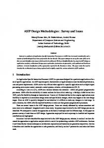
in terms of either bias because of the finite size of the training sample (86,87) or variance resulting from the same limitation. When this level is achieved, one has obtained the appropriate number of cases needed for training, and algorithm testing may proceed. Without much prior experience, it is difficult to know when that point is being approached. Hence, early in the developmental stages of computer-assist algorithms, it is necessary to consider that the finite training sample contributes to uncertainty in algorithm assessment as well as the finite test sample and their respective interactions, as discussed previously. Moreover, the dependencies of these effects on training and test sample numbers are not symmetric (84), therefore no simple rules for estimating target numbers are yet known. In the absence of prior experience with the task and populations of interest, a pilot study can be conducted and analyzed within the above framework to obtain estimates of the strengths of the variance components (46,78 – 81). One can then use the variance observed in the pilot study, together with estimates of the components and some basic rules for variances scaling, to estimate the size of training sets and the size of independent test sets required to obtain the uncertainties or error bars desired by users of the final database. A different way to state these concepts is the following. The components of variance quantify the variability of training and test set difficulty in the database as seen through the competing algorithms and estimated with the finite samples available, which is the information required for a quantitative estimate of a target size for the database. A pilot study should be sufficiently sized to obtain reliable estimates of the variance components. One advantage of the approach of Beiden et al (81– 83) is that it also provides estimates of the uncertainties associated with the variance components estimates themselves (83). If the resulting uncertainties are large, a corresponding safety factor for the target size of the database will be necessary. Sizing the pilot study itself is usually an exercise dominated by practical realities and the experiences of the investigators. Again, we emphasize that the entire discussion of variability here assumes that the investigators are sampling the specified target population without bias. Components of variance.—In Figure 1, we provide a sketch of the process of taking a multiple-reader, multiple-case, multiple-modality data set and decomposing it into the components of variance described earlier. An attractive feature of the process exhibited in this figure is that any of the assessment paradigms discussed previously

Academic Radiology, Vol 11, No 4, April 2004

Figure 1. Fundamental framework for multiple-reader (MR), multiple-case (MC) data. The black box may contain any accuracy measure such as Se, Sp, AUC, partial AUC, or corresponding summary measures of location-specific ROC paradigms. When truth is unavailable, the ROC-without-truth or RPA paradigms may be used to replace the ROC measures.

can be swapped into the “black box” to replace the conventional ROC paradigm. For example, any of the location-specific versions of the ROC paradigm may replace the conventional ROC one (software available at http:// www.radiology.arizona.edu/krupinski/mips/rocprog.html). In the absence of truth, the ROC-without-truth paradigm or the Polansky-Kundel RPA paradigm may replace the conventional ROC paradigm. In any case, the six components of variance may be obtained via the Beiden et al (78 – 81) approach (82) and used to appreciate the relative contributions of each of these to the resulting uncertainty or error bars. Once the variances have been obtained, they may also be used for sizing a larger trial from the results of a pilot study. SUMMARY AND CONCLUSIONS Prospective planning of a database such as the LIDC database requires a reasonable understanding of its potential applications. LIDC planning is complicated by issues specific to lung cancer screening and diagnosis, such as the presence of multiple lesions that radiologists may wish to localize. In cases in which localization within a region (eg, a lobe) is sufficient, an ROI approach as described by Obuchowski et al (50) is valid. However, if

LIDC: ASSESSMENT METHODS & STATISTICAL ISSUES

image-guided therapies become a reality, more precise nodule localization will become critical. Location-specific techniques such as AFROC (41) offer alternatives, although they have noted limitations. An additional complication encountered is the difficulty of obtaining “truth”. There is no substitute for goldstandard verification of diagnosis. Methods proposed for evaluating performance without “truth” have limitations. Truth will be available only on some subsets within the database. The lack of a verified diagnosis on all cases in the database raises the issue of verification bias. Without pathologic truth, consensus by a panel of expert radiologists may be the best source of “truth” data, which may introduce further uncertainty beyond that in the truthknown case. Investigators might use estimation techniques to attempt to fit the truth and then proceed with classical assessment paradigms, but such an approach can be misleading. Alternatively, they might use RPA, with and without the computer. Each of these approaches is problematic and thus requires further investigation to understand its quantitative limitations. For a given application, the number of images necessary to adequately power the database is complex as it depends on the task, the complexity of the algorithm and multiple sources of variability. We reviewed important considerations about bias and discussed the variability associated with training and testing datasets. An isomorphism between the MRMC paradigm in imaging provides a model to account for the sources of variability. In summary, we have given a brief review of some of the issues that have been discussed by the LIDC in connection with assessment methods that users of the database may wish to consider and that the LIDC itself must consider as it moves forward with the creation of a database resource for the medical imaging research community. The LIDC is actively engaged in further understanding the complexities of the statistical issues discussed here and the manner in which these issues will impact the eventual utility of the database. This review is meant only as a point of departure for further discussion by investigators; it is far from a complete treatment of this rich and evolving field. More specifically, it is meant to be descriptive, not prescriptive. We hope that the existence of the LIDC database will provide opportunities for investigators to push to new levels the frontiers of methodological issues and statistical solutions.

473

DODD ET AL

The Lung Image Database Consortium is: Samuel G. Armato III, Ph.D.1, Geoffrey McLennan, M.D.2, Michael F. McNitt-Gray, Ph.D.3, Charles R. Meyer, Ph.D.4, David Yankelevitz, M.D.5, Denise R. Aberle, M.D.3, Claudia I. Henschke, M.D., Ph.D.5, Eric A. Hoffman, Ph.D.2, Ella A. Kazerooni, M.D., M.S.4, Heber MacMahon, M.D.1, Anthony P. Reeves, Ph.D.5, Barbara Y. Croft, Ph.D.6, Laurence P. Clarke, Ph.D.6, Lori E. Dodd, Ph.D.6, David Gur, Sc.D.7, Nicholas A. Petrick, Ph.D.8, Edward Staab, M.D.6, Daniel C. Sullivan, M.D.6, Robert F. Wagner, Ph.D.8, Peyton H. Bland, Ph.D.4, Keith Brautigam, B.A.2, Matthew S. Brown, Ph.D.3, Barry De Young, M.D.2, Roger M. Engelmann, M.S.1, Andinet A. Enquobahrie, M.S.5, Carey E. Floyd, Jr., Ph.D.9, Junfeng Guo, Ph.D.2, Aliya N. Husain, M.D.1, Gary E. Laderach, B.S.4, Charles E. Metz, Ph.D.1, Brian Mullan, M.D.2, Richard C. Pais, B.S.3, Christopher W. Piker, B.S.2, James W. Sayre, Dr.PH.3, Adam Starkey1 REFERENCES 1. Jemal A, Murray T, Samuels A, Ghafoor A, Ward E, Thun MJ. Cancer statistics 2003. CA Cancer J Clin 2003; 53:5–26. 2. Fry WA, Menck HR, Winchester DP. The National Cancer Data Base report on lung cancer. Cancer 1996; 77:1947–1955. 3. Martini N, Bains MS, Burt ME, et al. Incidence of local recurrence and second primary tumors in resected stage I lung cancer. J Thorac Cardiovasc Surg 1995; 109:120 –129. 4. Flehinger BJ, Kimmel M, Melamed M. The effect of surgical treatment on survival from early lung cancer. Chest 1992; 101:1013–1018. 5. Kaneko M, Eguchi K, Ohmatsu H, et al. Peripheral lung cancer: screening and detection with low-dose spiral CT versus radiography. Radiology 1996; 201:798 – 802. 6. Henschke CI, McCauley DE, Yankelevitz DF, et al. Early Lung Cancer Action Project: overall design and findings from baseline screening. Lancet 1999; 354:99 –105. 7. Sone S, Takashima S, Li F, et al. Mass screening for lung cancer with mobile spiral computed tomography scanner. Lancet 1998; 351:1242– 1245. 8. Ohmatsu H, Kakinuma R, Kaneko M, Moriyama N, Kusumoto M, Eguchi K. Successful lung cancer screening with low-dose helical CT in addition to chest x-ray and sputum cytology: the comparison of two screening period with or without helical CT. Radiology 2000; 217(P): 242(abstr). 9. Rubin GD. Data explosion: The challenge of multidetector-row CT. Eur J. Radiol 2000; 36:74 – 80. 10. Naidich DP. Helical computed tomography of the thorax: clinical applications. Radiol Clin North Am 1994; 32:759 –774. 11. Clarke LP, Croft BY, Staab E, Baker H, Sullivan DC. National Cancer Institute initiative: Lung image database resource for imaging research. Acad Radiol 2001; 8:447– 450. 12. Giger ML. Current issues in CAD for Mammography. In: Doi K, Giger ML, Nishikawa RM, Schmidt RA, eds. Proceedings of the 3rd International Workshop on Digital Mammography, Digital Mammography ’96. Amsterdam: Elsevier, 1996; 53–59.

1The

University of Chicago, 2University of Iowa, 3University of California, Los Angeles, 4University of Michigan, 5Cornell University, 6National Cancer Institute, 7University of Pittsburgh, 8Food and Drug Administration, 9Duke University.

474

Academic Radiology, Vol 11, No 4, April 2004

13. Schultz DG, Wagner RF, Campbell G. Editorial response. Radiology 1997; 202:317–318. 14. Wagner RF, Beiden SV, Campbell G, Metz CE, Sacks WM. Assessment of medical imaging and computer-assist systems: Lessons from recent experience. Acad Radiol 2002; 9:1264 –1277. 15. Swets JA, Pickett RM. Evaluation of diagnostic systems. New York: Academic Press, 1982. 16. Metz CE. Basic principles of ROC analysis. Semin Nucl Med 1978; 8:283–298. 17. Metz CE. ROC methodology in radiologic imaging. Invest Radiol 1986; 21:720 –733. 18. Metz CE. Some practical issues of experimental design and data analysis in radiological ROC studies. Invest Radiol 1989; 24:234 –245. 19. Metz CE. Fundamental(s) of ROC Analysis. In: Handbook of Medical Imaging. Beutel J, Kundel HL, Van Metter RL, eds. Physics and Psychophysics. Vol 1. Bellingham, WA: SPIE Press, 2000, 751–769. 20. Wagner RF, Beiden SV, Metz CE. Continuous versus categorical data for ROC analysis: some quantitative considerations. Acad Radiol 2001; 8:328 –334. 21. Metz CE. Statistical analysis of ROC data in evaluating diagnostic performance. In: Herbert DE, Myers RH, eds. Multiple regression analysis: applications in the health sciences. New York: American Institute of Physics: American Association of Physicists in Medicine, 1986; 365– 384. 22. Metz CE, Herman BA, Shen JH. Maximum likelihood estimation of receiver operating characteristic (ROC) curves from continuously-distributed data. Stat Med 1998; 17:1033–1053. 23. Pepe MS. An interpretation for the ROC curve and inference using GLM procedures. Biometrics 2000; 56:352–359. 24. Zou KH, Hall WJ. Two transformation models for estimating an ROC curve derived from continuous data. J Appl Stat 2000; 27:621– 631. 25. Shapiro DE. The interpretation of diagnostic tests. Stat Methods Med Res 1999; 8:113–134. 26. Tosteson AA, Begg CB. A general regression methodology for ROC curve estimation. Med Dec Making 1988; 8:204 –215. 27. Toledano AY, Gatsonis C. Ordinal regression methodology for ROC curves derived from correlated data. Stat Med 1996; 15:1807–1826. 28. Cai T, Pepe MS. Semiparametric receiver operating characteristic analysis to evaluate biomarkers for disease. J Am Stat Assoc 2002; 97:1099 –1107. 29. Dodd LE, Pepe MS. Semi-parametric regression for the area under the receiver-operating characteristic curve. J Am Stat Assoc 2003; 98:397– 405. 30. Dodd LE, Pepe MS. Partial AUC estimation and regression. Biometrics 2003 Sep; 59:614 – 623. 31. Pepe MS. An interpretation for the ROC curve and inference using GLM procedures. Biometrics 2000; 56:352–359. 32. Nishikawa RM, Yarusso LM. Variations in measured performance of CAD schemes due to database composition and scoring protocol. Proc SPIE 1998; 3338:840 – 844. 33. Giger ML. Current issues in CAD for mammography. In: Doi K, Giger ML, Nishikawa RM, Schmidt RA, eds. Digital mammography ’96. Philadelphia: Elsevier Science, 1996; 53–59. 34. Bunch PC, Hamilton JF, Sanderson GK, Simmons AH. A free response approach to the measurement and characterization of radiographic observer performance. Proc SPIE 1977; 127:124 –135. 35. Chakraborty DP. Maximum likelihood analysis of free-response receiver operating characteristic (FROC) data. Med Phys 1989; 16:561– 568. 36. Chakraborty DP, Winter L. Free-response methodology: alternate analysis and a new observer-performance experiment. Radiology 1990; 174:873– 881. 37. Metz CE, Starr SJ, Lusted LB. Observer performance in detecting multiple radiographic signals: prediction and analysis using a generalized ROC approach. Radiology 1976; 121:337–347. 38. Starr SJ, Metz CE, Lusted LB, Goodenough DJ. Visual detection and localization of radiographic images. Radiology 1975; 116:533–538. 39. Swensson RG. Unified measurement of observer performance in detecting and localizing target objects on images. Med Phys 1996; 23: 1709 –1725.

Academic Radiology, Vol 11, No 4, April 2004

40. Swensson RG. Using localization data from image interpretations to improve estimates of performance accuracy. Med Decis Making 2000; 20:170 –185. 41. Chakraborty DP. The FROC, AFROC and DROC variants of the ROC analysis. In: Beutel J, Kundel HL, Van Metter RL, eds. Handbook of medical imaging. Vol 1. Physics and psychophysics. Bellingham, WA: SPIE Press, 2000, 771–796. 42. Petrick N, Sahiner B, Chan H-P, Helvie MA, Paquerault S, Hadjiiski LM. Breast cancer detection: evaluation of a mass-detection algorithm for computer-aided diagnosis: experience in 263 patients. Radiology 2002; 224:217–224. 43. Metz CE. Evaluation of digital mammography by ROC analysis. In: Doi K, Giger M, Nishikawa R, Schmidt RA, eds. Digital mammography ’96. Amsterdam, The Netherlands: Elsevier Science, 1996; 61– 68. 44. Metz CE. Evaluation of CAD methods. In: Doi K, MacMahon H, Giger ML, Hoffmann KR, eds. Computer-aided diagnosis in medical imaging. Excerpta Medica International Congress Series, Vol. 1182. Amsterdam: Elsevier Science, 1999, 543–554. 45. Chakraborty DP. Statistical power in observer performance studies: comparison of the receiver operating characteristic and free-response methods in tasks involving localization. Acad Radiol 2002; 9:147–156. 46. Dorfman DD, Berbaum KS, Metz CE. Receiver operating characteristic rating analysis: generalization to the population of readers and patients with the jackknife method. Invest Radiol 1992; 27:723–731. 47. Roe CA, Metz CE. Dorfman-Berbaum-Metz method for statistical analysis of multireader, multimodality receiver operating characteristic data: validation with computer simulation. Acad Radiol 1997; 4:298 –303. 48. Chakraborty DP, Berbaum KS. Comparing inter-modality diagnostic accuracies in tasks involving lesion localization: a jackknife AFROC approach. Radiology 2002; 225(Suppl P):259. 49. Chakraborty, DP. Proposed solution to the FROC problem and an invitation to collaborate. In: Chakraborty, DP, Krupinski, EA, (eds.), Medical imaging 2003: image perception, observer performance, and technology assessment, Vol 5034, Proc SPIE, 204 –212 50. Obuchowski NA, Lieber ML, Powell KA. Data analysis for detection and localization of multiple abnormalities with application to mammography. Acad Radiol 2000; 7:516 –525. 51. Rutter CM. Bootstrap estimation of diagnostic accuracy with patientclustered data. Acad Radiol 2000; 7:413– 419. 52. Efron B, Tibshirani RJ. An introduction to the bootstrap. New York: Chapman and Hall, 1993. 53. Chakraborty D, Obuchowski NA, Lieber ML, Powell KA. Point-counterpoint. Acad Radiol 2000; 7:553–556. 54. Begg CB, Greenes RA. Assessment of diagnostic tests when disease verification is subject to selection bias. Biometrics 1983; 39:207–215. 55. Gray R, Begg CB, Greenes RA. Construction of receiver operating characteristic curves when disease verification is subject to selection bias. Med Decis Making 1984; 4:151–164. 56. Zhou XH. Correcting for verification bias in studies of a diagnostic test’s accuracy. Stat Methods Med Res 1998; 7:337–353. 57. Revesz G, Kundel HL, Bonitatibus M. The effect of verification on the assessment of imaging techniques. Invest Radiol 1983; 18:194 –198. 58. Walter SD, Irwig LM. Estimation of test error rates, disease prevalence and relative risk from misclassified data: a review. Clin Epidemiol 1988; 41:923–937. 59. Vacek PM. The effect of conditional dependence on the evaluation of diagnostic tests. Biometrics 1985; 41:959 –968. 60. Torrance-Rynard VL, Walter SD. Effects of dependent errors in the assessment of diagnostic test performance. Stat Med 1997; 97:2157–2175. 61. Qu Y, Tan M, Kutner MH. Random effects models in latent class analysis for evaluating accuracy of diagnostic tests. Biometrics 1996; 52: 707– 810. 62. Espeland MA, Handleman SL. Using latent class models to characterize and assess relative-error in discrete measurements. Biometrics 1989; 45:587–599. 63. Hui SL, Zhou XH. Evaluation of diagnostic tests without a gold standard. Stat Methods Med Res 1998; 7:354 –370. 64. Albert PS, McShane LS, Shih JH. Latent class modeling approaches for assessing diagnostic error without a gold standard: with applica-

LIDC: ASSESSMENT METHODS & STATISTICAL ISSUES

65.

66.

67. 68. 69.

70. 71.

72.

73.

74.

75. 76.

77. 78.

79.

80.

81.

82.

83. 84.

85. 86.

87.

tions to p53 immunohistochemical assays in bladder tumors. Biometrics 2001; 57:610 – 619. Albert PS, Dodd LE.A cautionary note on the robustness of latent class models for estimating diagnostic error without a gold standard. (submitted) Dendukuri NM, Lawrence JL. Bayesian approaches to modeling the conditional dependence between multiple diagnostic tests’. Biometrics 2001; 57:158 –167. Henkelman RM, Kay I, Bronskill MJ. Receiver operator characteristic (ROC) analysis without truth. Med Decis Making 1990; 10:24 –29. Begg CB, Metz CE. Consensus diagnoses and “gold standards”. Med Decis Making 1990; 10:29 –30. Beiden SV, Campbell G, Meier KL, Wagner RF. On the problem of ROC analysis without truth: the EM algorithm and the information matrix. Proc SPIE 2000; 3981:126 –134. University of Chicago ROC software. Available at: http://wwwradiology.uchicago.edu/krl/toppage11.htm#software. Metz CE, Wang PL, Kronman HB. A new approach for testing the significance of differences between ROC curves measured from correlated data. In: Deconinck F, ed. Information processing in medical imaging. The Hague: Nijhoff, 1984; 432– 445. Kundel HL, Polansky M. Comparing observer performance with mixture distribution analysis when there is no external gold standard. Proc SPIE 1998; 3340:78 – 84. Polansky M. Agreement and accuracy mixture distribution analysis. In: Handbook of medical imaging. Beutel J, Kundel HL, Van Metter RL, eds. Physics and psychophysics Vol 1. Bellingham, WA: SPIE Press, 2000, 797– 835. Kundel HL, Polansky M, Phelan M. Evaluating imaging systems in the absence of truth: a comparison of ROC and mixture distribution analysis in computer aided diagnosis in mammography. Proc SPIE 2000; 4324:22. Hastie T, Tibshirani RJ, Friedman JThe elements of statistical learningdata mining, inference and prediction. New York: Springer-Verlag, 2001. Kundel HL, Polansky M. Comparing observer performance with mixture distribution analysis when there is no external gold standard. Proc SPIE 1998; 3340:78 – 84. Begg CB, NcNeil BJ. Assessment of radiologic tests: control of bias and other design considerations. Radiology 1988; 167:565–569. Beiden SV, Maloof MA, Wagner RF. A general model for finite-sample effects in training and testing of competing classifiers. IEEE Trans Patt Anal Mach Intel 2003; 25:1561–1569. Beiden SV, Wagner RF, Campbell G. Components-of-variance models and multiple-bootstrap experiments: an alternative method for random-effects receiver operating characteristic analysis. Acad Radiol 2000; 7:341–349. Beiden SV, Wagner RF, Campbell G, Metz CE, Jiang Y. Components-ofvariance models for random-effects ROC analysis: the case of unequal variance structures across modalities. Acad Radiol 2001; 8:605– 615. Beiden SV, Wagner RF, Campbell G, Chan H-P. Analysis of uncertainties in estimates of components of variance in multivariate ROC analysis. Acad Radiol 2001; 8:616 – 622. Wagner RF, Beiden SV, Campbell G. Multiple-reader studies, digital mammography, computer-aided diagnosis–and the Holy Grail of imaging physics (I). Proc SPIE 2001; 4320:611– 618. Obuchowski NA. Multireader receiver operating characteristic studies: a comparison of study designs. Acad Radiol 1995; 2:709 –716. Gatsonis CA, Begg CB, Wieand S. Advances in statistical methods for diagnostic radiology: a symposium. Acad Radiol 1995; 2(suppl 1):S1– S84. Gifford HC, King MA. Case sampling in LROC: a Monte Carlo analysis. Proc SPIE 2001; 4324:143–152. Chan H-P, Sahiner B, Wagner RF, Petrick N. Classifier design for computer-aided diagnosis: effects of finite sample size on the mean performance of classical and neural network classifiers. Med Phys 1999; 26:2654 –2668. Sahiner B, Chan H-P, Petrick N, Wagner RF, Hadjiiski L. Feature selection and classifier performance in computer-aided diagnosis: the effect of finite sample size. Med Phys 2000; 27:1509 –1522.

475