Arch. Mech., 65, 2, pp. 97–129, Warszawa 2013
Assessment of implementation variants of conditional scalar dissipation rate in LES-CMC simulation of auto-ignition of hydrogen jet A. TYLISZCZAK Institute of Thermal Machinery Faculty of Mechanical Engineering and Computer Science Częstochowa University of Technology Al. Armii Krajowej 21 42-200 Częstochowa, Poland e-mail:
[email protected] In this paper the large eddy simulation (LES) and conditional moment closure (CMC) combustion model have been applied for modelling of auto-ignition of hydrogen jet issuing into a hot ambient co-flow. Most of the attention was devoted to modelling aspects of the conditional scalar dissipation rate which is a key quantity of the CMC model. Two models are compared with emphasis on differences in distributions in mixture fraction space. Analysis of mutual relations between the terms of CMC equations confirms importance of the conditional scalar dissipation rate. It is also shown that model constants are crucial from the point of view of an autoignition location and a flame lift off height. The numerical results are compared with experimental data and both the mean and the root mean square fluctuating values of the temperature and species mass fraction agree well with measurements. Key words: auto-ignition, lifted flame, large eddy simulation, conditional moment closure. c 2013 by IPPT PAN Copyright !
1. Introduction Auto-ignition of gaseous mixture followed by a flame propagation and stabilisation are crucial from the point of view of safety, reliability and efficiency of many technical devices. Experimental analysis of auto-ignition is extremely difficult and expensive as it requires very sophisticated experimental apparatus and dedicated measurements techniques. On the other hand, today’s computers and available numerical tools enable modelling of these phenomena at reasonable time with acceptable accuracy. In contemporary CFD (computational fluid dynamics), in the field of combustion, the numerical modelling of strongly unsteady phenomena, such as ignition, local extinction or blow-off, is one of the most important and most difficult tasks. In non-premixed configurations the experimental and numerical studies concerning the auto-ignition have mainly
98
A. Tyliszczak
focused on gaseous fuels in simple configurations, such as mixing layers [1, 2], jet flows [3, 4, 5] or counter-flows [6, 7]. These research examined various fuels including hydrogen, pure or hydrogen-enriched methane, kerosene as aviation fuel, and other single component hydrocarbons. Mostly the research concentrated on parameters that prohibit or promote the auto-ignition phenomena. From this point of view, the scalar dissipation rate (or critical strain rate), equivalence ratio and temperature are regarded to be the most important [8]. In case of the laminar flows the general observation is that there exists some critical value of the scalar dissipation rate above which the auto-ignition does not occur. In case of the turbulent flows the situation may be different, i.e., even if the timeaveraged scalar dissipation rate is higher than the critical value the auto-ignition may still occur depending on the amplitude of fluctuations which may allow an excursion into a region of low scalar dissipation rate and last long enough to permit auto-ignition. On the other hand, even if the time-averaged scalar dissipation rate is smaller than the critical value the auto-ignition may be precluded because of long lasting excursions above that value [8]. In this paper we deal with a simple hydrogen jet issuing into a hot ambient flow. If the temperature of that flow is high enough then at some distance from the nozzle the jet spontaneously auto-ignites. In the numerical simulations this scenario takes place provided that the combustion model and all related submodels properly reflect the physics. As will be shown in the paper this is not always the case and at some point the combustion models must be tuned in order to predict the solution correctly. The paper concentrates on modelling aspects of the scalar dissipation rate as a key parameter of the conditional moment closure (CMC) model [9] and also all flamelet type models [10, 11, 12]. The focus is on the CMC model which together with Eulerian PDF approach [13, 14, 15, 16] is currently regarded as the most accurate. It allows for analysis of very complicated physical processes including lifted flames [17, 5], local extinction [18, 19], autoignition [20] or forced ignition [21, 22, 23]. All these phenomena are undoubtedly strongly unsteady and require precise and time accurate solutions. This is offered by the large eddy simulation (LES) method which is becoming a standard tool in academic research in virtually all aspects of fluid flow and related processes. The LES approach, contrary to the classical (u)RANS ((unsteady) Reynoldsaveraged Navier–Stokes) methods, gives a very deep insight into the unsteady turbulent flow phenomena. In case of fundamental research the LES method combined with the CMC model is very attractive as it enables an accurate analysis of basic physical processes. A big disadvantage of the CMC model is a very high computational cost from the point of view of the memory requirements as well as the computational time. This is particularly true when the CMC model is combined with LES approach which requires numerical mesh much finer than in RANS methods.
Assessment of implementation variants of conditional scalar. . .
99
Hence, the LES-CMC simulations even for relatively simple problems always involve a number of optimisation steps which in many cases open the fields for simplifications and various modelling strategies. One of the main objectives of this work is to explore sensitivity of LES-CMC approach to implementation variants of the scalar dissipation rate in auto-igntion problem; to the author knowledge such an analysis was never done before. The paper is organised as follows: in the next section the presentation of LES and CMC methods is limited to basic ideas and appropriate papers are cited for interested readers; the main attention is paid to possible variants of modelling of the scalar dissipation rate which are then compared; in Section 3 numerical schemes and algorithms used in the LES and CMC codes are briefly characterised; the obtained results are presented in Section 4 which is followed by conclusions. 2. Mathematical modelling 2.1. LES formulation
In LES the scales of the turbulent flow are divided into the large scales, which are directly solved on a given numerical mesh, and the small scales (subgrid scales) which require modelling. This separation of scales is obtained by a spatial filtering defined as [24, 25] ! ¯ (2.1) f (x, t) = G(x − x! , ∆)f (x! , t)dx! , Ω
where f stands for arbitrary variable and G(x, ∆) is the filter function: " 1/∆3 for |x − x! | < ∆, ! (2.2) G(x − x ) = 0 otherwise, with a filter width ∆ = V ol1/3 , where V ol stands for a local mesh volume. In the variable density flows the Favre filtering is applied almost without exception. It is defined as f#(x, t) = ρf /ρ where ρ is the density. Applying the filtering procedure to the continuity equation and the Navier–Stokes give (2.3) (2.4)
#j ∂ ρ¯ ∂ ρ¯u + = 0, ∂t ∂xj
∂τijsgs #i u #j ∂τij ∂ p¯ ∂ ρ¯u #i ∂ ρ¯u + =− + + , ∂t ∂xj ∂xi ∂xj ∂xj
where ui are the velocity components, p is the pressure. The stress tensor of the resolved field τij and unresolved subgrid stress tensor τijsgs , resulting from the
A. Tyliszczak
100
filtering of the non-linear advection & $% ∂# uj ∂# ui + − (2.5) τij = µ ∂xj ∂xi
terms, are defined as ' uk 2 ∂# δij , τijsgs = ρ (# ui u #j − u( i uj ) , 3 ∂xk
where µ is the molecular viscosity determined from the Sutherland law. In this work, the subgrid tensor is modelled by eddy-viscosity type model [25] defined as τijsgs = 2µt Sij − τkk δij /3,
(2.6)
) ∂ uei ∂u ej * and the subgrid (or turbulent) viscosity is computed + where Sij = 12 ∂x ∂x j i according to model proposed by Vreman [26] given as + Bβ (2.7) µt = ρ¯C , αij αij where ∂# uj , ∂xi
βkl = ∆2 αmk αml ,
(2.8)
αij =
(2.9)
2 2 2 Bβ = β11 β22 − β12 + β11 β33 − β13 + β22 β33 − β23 ,
and with the model constant C = 2.5 × 10⁻² . The model of Vreman is very easy to implement and almost negligible from the point of view of additional computational cost. This model overcomes a weakness of the classical eddyviscosity type models which are known to be excessively dissipative near the walls. Similarly, as in the case of dynamic subgrid models [27] or in the WALE approach [28] the subgrid viscosity in the model of Vreman vanishes in pure shear regions. The CMC model presented in the next section belongs to the family of the mixture fraction based models [11]. The mixture fraction ξ measures the local fuel/oxidizer ratio and its standard definition is given as (2.10)
ξ=
sYF − YO + YO0 , sYF0 + YO0
where s is the mass stoichiometric ratio, the symbols YF and YO denote fuel and oxidizer mass fractions in a mixture and YF0 and YO0 are the fuel and oxidizer mass fractions in pure fuel and oxidizer streams, respectively. The mixture fraction varies in the range 0 ≤ ξ ≤ 1, and ξ = 0 (obtained with YF = 0, YO = YO0 ) denotes the mixture composition corresponding to the oxidizer composition, and ξ = 1 (YF = YF0 , YO = 0) corresponds to the fuel composition. The mixture
Assessment of implementation variants of conditional scalar. . . 101
fraction is a conserved quantity and it obeys the classical convection-diffusion transport equation, which in the framework of LES is defined as % & ∂Jsgs #i ξ# ∂ ∂ ξ# ∂ ρ¯ξ# ∂ ρ¯u + = ρ¯D + , (2.11) ∂t ∂xi ∂xi ∂xi ∂xi
where D = µ/¯ ρSc is the molecular diffusivity and Sc = 0.7 is the Schmidt e
∂ξ with the number. The term Jsgs is the subgrid part modelled as Jsgs = ρ¯Dt ∂x i subgrid diffusivity Dt = µt /¯ ρSct where the turbulent Schmidt number is assumed constant Sct = 0.4 [29].
2.2. CMC formulation
The CMC model has been formulated in 1990s by Klimenko and Bilger and then it was summarized in the joint paper [9]. In the context of LES the CMC model has been presented in [30] approximately ten years later, where it was derived applying the density-weighted conditional filtering operation [31, 30, 29] to the transport equations for the species (Yk ) mass fraction and total enthalpy (h). The final form of the CMC equations in the framework of LES is given as [30, 29] (2.12) (2.13)
∂Qh ∂ 2 Qh ∂Qh ( + u( =N |η + eh , i |η ∂t ∂xi ∂η 2
∂Qk ∂Qk ∂ 2 Qk ( + u( =N |η + ω( i |η k |η + eY , ∂t ∂xi ∂η 2
k = 1, 2, . . . , n,
where n is the number of reacting species. The operator (·|η) = (·|ξ = η) is the conditional filtering operator with conditioning being done on the mixture , fraction. The symbols Qk = Y( k |η and Qh = h|η are the conditionally filtered ( species mass fractions and enthalpy, u( i |η - velocity, N |η - scalar dissipation rate. The symbols eY , eh represent the subgrid interactions and they are usually expressed as [29, 20, 5] % & % & ∂Qk ∂ ∂Qh ∂ ( ( Dt |η Dt |η , eh = , (2.14) eY = ∂xi ∂xi ∂xi ∂xi ( where D t |η is the conditionally filtered subgrid diffusivity. The conditionally filtered reaction rate is evaluated with the first order closure [9] where the subgrid conditional fluctuations are neglected, i.e., ω( k |η = ωk (Q1 , Q2 , . . . , Qn , Qh ). The conditionally filtered variables are related to the filtered variables by the integration over the mixture fraction space, this is defined as (2.15)
f#(x, t) =
!1 0
f, |η P#(η)dη,
102
A. Tyliszczak
where P# is a filtered probability density function assumed here as a beta-function PDF defined as [32] (2.16)
P (ξ) = ξ a−1 (1 − ξ)b−1
Γ (a + b) , Γ (a)Γ (b)
!!2 − 1) , b = a(1 − ξ)/ # ξ(1 # − ξ)/ # ξ, # ξ, # Γ (x) is the gamma function where: a = ξ( !!2 is the filtered mixture fraction variance modelled as ξ, !!2 = C ∆2 ∂ ξe ∂ ξe . and ξ, V ∂xj ∂xj
The value of the parameter CV may be computed dynamically or may be a fixed constant [33, 34]. For simplicity here it is assumed that CV = 0.1, as suggested by [34]. From the point of view of the solution of the CMC equations the main difficulty is related to a very large computational cost. The CMC equations are formulated in the four dimensional space, i.e., physical co-ordinates and mixture fraction space. It means that in every time step the solution would have to be computed on Nx,y,z × Nη nodes, where Nx,y,z and Nη denote the number of nodes in the physical and mixture fraction spaces. This would imply the computational cost which would prevent using of the LES-CMC approach for realistic problems, and even in simple cases the computations would be hardly feasible. A number of optimisation and simplifications steps have to be performed to reduce huge memory requirements and very long simulation times. A common simplifying approach is to use two separate meshes in physical space: one for the solution of the flow field (CFD mesh) and another one, much coarser for the CMC equations (CMC mesh). In the papers cited above the ratio of the nodes of CFD/CMC meshes varies in between 20–300 depending on the flow problem. The application of the coarser mesh for the CMC model is justified by the fact that in physical space the conditionally filtered variables are smoother than the LES filtered variables [30]. Hence, they do not require the numerical resolution as good as for the flow variables (velocity, mixture fraction). The second difficulty of the CMC model is connected to the modelling of the conditional terms appearing in Eqs. (2.12) and (2.13), i.e., the conditionally filtered scalar dissipation rate, velocity and diffusivity. These terms have to be computed based on the resolved variables before solving the CMC equations. The conditional scalar dissipation rate N |η is usually computed applying the AMC – amplitude mapping closure model [35, 36, 37] defined as
(2.17)
( N |η = N0 G(η),
G(η) = exp(−2[erf −1 (2η − 1)]2 ), N0 = - 1 0
# N , G(η)P# (η)dη
Assessment of implementation variants of conditional scalar. . . 103
# is comwhere erf(x) is the error function. The filtered scalar dissipation rate N puted as the sum of the resolved and subgrid part [18, 30, 5]: (2.18)
/ # ∂ ξ# νt !!2 1 ∂ ξ # =D . + CN 2 ξ, N ∂xi ∂xi ∆ 3 02 12 0 12 3 subgrid .
resolved
The constant CN is an important parameter in flow problems which depend # and thus on N |η. Typical examples are flames with strongly on the level of N local extinction and re-ignition or auto-ignition phenomena. There are no clear recommendations on what value of CN should be in a particular problem, and thus the value of CN is sometimes estimated based on existing experimental or DNS data [38] and sometimes it is set by trial and error. Analysis of influence of CN on the results is discussed later in the paper (Section 4). The models for the conditionally filtered velocity and diffusivity are much simpler than for N |η. In many papers [30, 29, 20, 18] it is shown that on the ( level of CFD resolution the conditional terms u( i |η and Dt |η may be assumed ( equal to the filtered values, i.e., u( #i and D i |η ≈ u t |η ≈ Dt . This is the simplest approach and it is used in the present work. 2.3. Transfer between CFD and CMC mesh
The application of two meshes requires that the conditional terms that have been computed on the CFD mesh must be transferred to the CMC mesh. Various possibilities for transferring data between the CMC and CFD meshes have been discussed in [29]. Here, the formulas pointed as the most proper ones are used. Assuming that the conditional variable (f, |η) has been computed on the CFD mesh, its counterpart on the CMC mesh is determined by using a PDF weighted volume integral within the CMC cells (VCM C ) defined as (2.19)
∗
f, |η =
-
VCMC
-
ρ¯P# (η)f, |η dV ! ; ρ¯P#(η) dV !
VCMC
∗ thus, the conditionally filtered variable f, |η corresponding to the CMC cell is common for a group of the CFD nodes embedded in that CMC cell. The for∗ (∗ mula (2.19) is applied for velocity u( i |η , diffusivity Dt |η and also for the scalar ∗ ( dissipation rate N |η . However, in this case there is another option to com∗ ( pute N |η and it relies on application of the AMC model directly on the CMC resolution [29]. This approach leads to
104
(2.20)
A. Tyliszczak ∗ ( N |η = N0∗ G(η),
G(η) = exp(−2[erf −1 (2η − 1)]2 ), N0∗ = - 1 0
#∗ N , G(η)P# ∗ (η)dη
# ∗ and P# ∗ (η) are the volume integrated values: where N # dV ! ρ¯N ρ¯P#(η) dV ! V ∗ ∗ CMC # (η) = VCMC # = , P . (2.21) N ¯ dV ! ¯ dV ! VCMC ρ VCMC ρ
In this work we compare the results obtained with two variants of computing ∗ ( N |η . The variant defined by Eq. (2.17) with the volume integration according to Eq. (2.19) will be denoted as N-1, and the variant defined by Eq. (2.20) with Eq. (2.21) will be denoted as N-2. Here, one should realize that there are no ∗ ( physical aspects that led to different formulations for N |η on the CMC mesh – the differences come from the necessity of application of two separate meshes with different number of nodes. Actually, if the CMC and CFD meshes were equal then the variant N-1 and N-2 would become identical and consistent with Eq. (2.17). From the point of view of the computational time the variant N-2 is slightly less costly, mainly because the AMC model (Eq. (2.20)) is applied once for the CMC cell. However, the computational time needed for calculation of ∗ ( N |η has a minor contribution in a total computational time and therefore this aspect cannot be regarded as an important parameter in the evaluation of N-1 and N-2 variants. Finally, it is worth to mention that the volume integrals (2.21) are simplified form of Eq. (2.19), i.e., one could write: ρ¯f#dV ! V ∗ # (2.22) f = CMC ρ¯ dV ! VCMC
,t ∗ [29, 20]. and these forms are sometimes used when evaluating u #∗i and D Having all needed conditional terms computed the CMC equations can be solved. Next, the species and enthalpy on the CFD mesh are computed from ! 1 ∗ # (2.23) f (x, t) = f, |η P#(η)dη 0
∗ with P#(η) evaluated separately in each of the CFD nodes and with f, |η being the same for the group of the CFD nodes belonging to particular CMC cells.
Assessment of implementation variants of conditional scalar. . . 105
3. Numerical methods The CMC model has been implemented in a high-order LES solver called SAILOR. The SAILOR code is based on the low Mach number approach [39, 40]. The spatial discretisation is performed by the sixth order compact method [41] for the Navier–Stokes and continuity equations and with fifth order WENO scheme [42] for the mixture fraction. The time integration is performed by the Adams-Bashforth/Adams-Multon predictor-corrector approach. The solution algorithm is well verified, the SAILOR code was used in various LES studies for gaseous flows, multi-phase flows and flames [43, 44, 45, 46]. The type of applied high-order spatial discretisation limits applicability of the code to simple geometries such as channel or free jet flows. On the other hand, as the discretisation errors are minimized one may expect that the differences between applied models should be highlighted and easier to identify. This is the main advantage of using high-order schemes. The CMC equations were solved applying the operator splitting approach where the transport in physical space, transport in mixture fraction space and chemistry are solved separately. Time integration in physical space was performed with the first order explicit Euler method. In mixture fraction space the CMC equations are stiff due to the reaction rate terms. In this case the time integration had to be performed applying the VODPK [47] solver that is well suited for stiff systems. The CMC terms in mixture fraction space are: the source terms and the second derivatives of the species and enthalpy. These terms, i.e., ∂ 2 Qk,h /∂η 2 , were discretised using the second order finite difference method [48]. The reaction rates were computed using CHEMKIN interpreter [49]. The chemistry is modelled by Muller’s mechanism [50] with 9 species and 21 reactions. The CMC terms in physical space are the convective terms u( i |η(∂Qk,h /∂xi ) and the diffusive terms defined by (2.14). The conditional variables are smoother in physical space and therefore they were discretised with second order methods. The convective terms were discretized using second order TVD (total variation diminishing) [51] method with van Leer’s [52] limiters. The diffusive terms were discretised using the central finite difference scheme. 4. Computational results A sketch of the computational configuration is shown in Fig. 1, it corresponds to the test case studied experimentally and numerically in [3]. The fuel jet is a mixture of hydrogen and nitrogen with the molar fraction XH2 = 0.254, XN2 = 0.746. The fuel temperature is 305 K, the mean velocity at the nozzle exit is equal to U = 107 m/s, and the nozzle diameter is D = 4.57 mm. The fuel
106
A. Tyliszczak
Fig. 1. Schematic view of the computational configuration for auto-ignition of H2 /N2 jet.
jet auto-ignites due to the presence of hot co-flowing stream. Its temperature is equal to Tc = 1045 K ± 3%, the velocity of the co-flow is equal to Uc = 3.5 m/s and the ambient pressure is assumed equal to the atmospheric pressure. The co-flow mixture consists of the oxygen XO2 = 0.147, water XH2 O = 0.1 and nitrogen XN2 = 0.753. The stoichiometric composition corresponds to the mixture fraction ξST = 0.476, and the most reactive mixture fraction, i.e., where the auto-ignition occurs in mixture fraction space [8], equals to ξM R = 0.0534. The auto-ignition time and a final flame position are sensible to Tc [4, 53, 54, 55]. For higher values of Tc the jet auto-ignites quickly, the flame propagates downstream and attaches to the nozzle eventually. For lower values of Tc , the flame remains lifted and the lift off height H is a function of Tc . The lift off height was determined as the axial distance form the nozzle where the mass fraction of species OH increased up to 2×10⁻⁴ . In [3] for the co-flow temperature Tc = 1045 K they observed H/D ≈ 10, both in the computations and in the experimental data. On the other hand in [54], applying LES with Eulerian PDF approach, the same lift off height was obtained for Tc = 1035 K, which however, lies in the 3% error bar of the temperature measurements [3]. Additionally in [54] they stressed that this test case is particularly sensitive to Tc and even a few degrees of variation may play an important role. 4.1. Solutions in physical space
In this work the computations were performed for Tc = 1030 K, Tc = 1035 K and Tc = 1045 K. The computational domain was the rectangular box with dimensions 15D × 15D × 35D in x, y and z direction respectively. Two sets of the
Assessment of implementation variants of conditional scalar. . . 107
LES and CMC meshes were used: (i) coarse configuration with 128 × 128 × 196 nodes for LES solver and 23 × 23 × 60 nodes for the CMC model; (ii) refined configuration with 140 × 140 × 240 and 23 × 23 × 90 nodes, respectively for LES and CMC part. In both cases the meshes were smoothly stretched towards the nozzle, both axially (z-direction) and in the directions x, y. In the region of the jet the meshes were nearly uniform in the directions x, y. The minimum cell sizes of the refined LES mesh were ∆xmin = ∆ymin = 0.048D and ∆zmin = 0.087D. Close to the outlet the maximum cell size in z-direction was equal to ∆zmax = 0.223D. The time step for all the simulations was equal to ∆t = 5 × 10⁻⁷ s what corresponded to the CFL number equal approximately to 0.5. The inlet boundary conditions for the velocity are: fully developed pipe flow for the jet and the uniform velocity profile for the co-flow. The velocity fluctuations were added to the mean profile according to the digital filtering method [56]. The pressure was computed based on the Neumann condition ∂p/∂n = 0. The mixture fraction at the inlet was specified as: ξ = 1 (corresponding to XH2 = 0.254, XN2 = 0.746) for the jet, and ξ = 0 (corresponding to XO2 = 0.147, XH2 O = 0.1, XN2 = 0.753) for the co-flow. In mixture fraction space the solution was assumed as inert, i.e., the enthalpy and species for ξ ∈ (0, 1) varied linearly. On the side boundaries the velocity was equal to the co-flow velocity, the pressure and the other variables where computed applying the Neumann boundary conditions. At the outlet boundary the pressure was constant and the remaining variables were computed from the Orlansky type convective condition [57]: ∂f /∂t + U ∂f /∂n = 0, with the convection velocity U corresponding to the mean normal velocity at the outlet. The simulations were performed on a PC cluster using 20 CPU cores (Intel Xeon 2.67 GHz). The computational cost of the simulation was dependent on the flow conditions (before auto-ignition, flame propagation, developed attached or lifted flame) and was the biggest for the fully developed flame. In this case, the computations of 0.01 s of physical time required approximately 8 days of the continuous simulation. The time-averaged results (presented in Section 4.3) were collected for approximately 0.01 s starting from the time when the flame was developed. The averaging time corresponded to slightly more than 6.5 passes of the flow through the flow domain (assuming the uniform jet velocity as the reference velocity). The obtained results were practically independent of the mesh density and minor differences were only visible in the time-averaged data. Similarity of the solutions obtained on different meshes was attributed to the high-order discretization method which is assumed to yield the grid independent results at relatively small number of the nodes. Theoretically, this never happens in LES method as the filter width is related to the mesh density. All the results presented in the following sections were obtained using the refined configuration of the meshes.
108
A. Tyliszczak
The following analysis concentrates on a comparison of two variants of com∗ ( puting N |η which in the previous section were denoted as Variant N-1 and ∗ ( # that requires setting Variant N-2. In both the cases N |η is evaluated using N the model constant CN . As it was mentioned in the previous section there is no clear recommendation what a value this constant should have. For example in LES-CMC simulations of an auto-ignition of hydrogen jet [20, 5] or a bluff-body stabilised methane flame [21] it was assumed that CN = O(1), whereas in [18] for a methane flame with local extinctions (Sandia F) CN was equal to 42, as a result of calibration based on experimental data. Furthermore, an analysis pre# sented in [38], performed based on DNS solutions, shows that subgrid part of N varies considerably and its correct prediction may require tuning of the model constant. The preliminary computations were performed with the constant CN = 2 which was the same as in [5]. The obtained results for variant N-1 and variant N-2 show that after the occurrence of autoignition the flame propagates towards the nozzle (inlet plane) and remains nearly attached to the nozzle for all analysed co-flow temperatures. Sample evolution of the flame for Tc = 1030 K starting form the auto-ignition phase, up to the fully developed flame, is shown in Figs. 2–5, these results were obtained applying variant N-1. The presented contours show the temperature and radicals OH and HO2 . The white lines in the figures with the temperature contours correspond to the stoichiometric mixture fraction. In the time instant T1 = 3 × 10⁻³ s the temperature is low but the first signs of the auto-ignition are already seen. This is manifested by an increase of HO2 , which is called the pre-ignition species [8], and regarded as the indicator of the flame appearance. In the next time steps the radicals OH are visible at H/D ≈ 5, the temperature increases rapidly and the flame starts to propagate downstream. Eventually it stabilises very close to the inlet, in the third CMC cell. In the present case, the flame will never fully attach to the inflow plane because of the assumed inert boundary condition. Figure 6 shows the isosurfaces of the temperature and the mixture fraction inside the flame. Here it is well seen that the high temperature regions are in the mixing layer and they occur very close to the inlet. The auto-ignition scenario for Tc = 1035 K and Tc = 1045 K is basically the same. In these cases the flame appears slightly faster, in the sense of the simulation time, but the final state is exactly the same as for Tc = 1030 K. Unfortunately all these results are inconsistent with the experimental data where the flame remained lifted at about H/D ≈ 10 for Tc = 1045 K. The computations performed for Tc = 1030 K, which is still in the 3% measurement error [3], should definitely yield to the lifted flame, at least a few diameters. 4.1.1. Results with standard model constant.
Assessment of implementation variants of conditional scalar. . . 109
Fig. 2. Contours of the temperature and mass fraction of OH and HO2 at time instant T1 = 3 × 10⁻³ s – beginning of the auto-ignition. Results obtained when applying variant N-1 with CN = 2.
Fig. 3. Contours of the temperature and mass fraction of OH and HO2 at time instant T2 = 5 × 10⁻³ s – production of OH. Results obtained when applying variant N-1 with CN = 2.
110
A. Tyliszczak
Fig. 4. Contours of the temperature and mass fraction of OH and HO2 at time instant T3 = 6 × 10⁻³ s – destruction of HO2 starting from z/D = 15. Results obtained when applying variant N-1 with CN = 2.
Fig. 5. Contours of the temperature and mass fraction of OH and HO2 at time instant T4 = 7 × 10⁻³ s – developed flame. Results obtained when applying variant N-1 with CN = 2.
Assessment of implementation variants of conditional scalar. . . 111
Fig. 6. Isosurfaces of the temperature (figure on the left-hand side) and mixture fraction inside the flame. Results obtained when applying variant N-1 with CN = 2.
Following the suggestions from [18], the next computations were performed with a higher value of CN , i.e., with CN = 40. Although it was much higher than the initial value CN = 2, one should note that it was more or less the same as in [18], where for the methane flame CN = 42 was used. Figure 7 shows the instantaneous solution for Tc = 1030 K, these results were obtained applying variant N-1. The flame is lifted at 4D approximately and even though this is still less than in the experiment it clearly shows the influence of CN modification. The results for Tc = 1035 K and Tc = 1045 K are very similar and the lift off height is practically the same. This may suggest that the influence of co-flow temperature is not as significant as stressed in [54], at least in the analysed range of temperatures. The present observations are rather consistent with analysis presented in [58] where it was concluded that the lift off height predicted by computations is mainly influenced by a turbulence model. Indeed, this seems to be confirmed by the following results obtained with variant N-2. Different values of the scalar dissipation rate resulting from the variant N-2 may be regarded as the effect of application of another turbulence model. The obtained solution shows that the flame stabilises closer to the inlet. The contours of time-averaged mass fraction of OH for Tc = 1030 K and Tc = 1035 K are presented in Fig.8, and though the averaging period Tave = 200D/U ≈ 8.5 ms was not long enough to obtain expected symmetric contours, the differences between the results achieved when applying variant N-1 and N-2 are evident. They are much more pronounced than differences caused by different co-flow temperatures. Indeed, the lift off height for Tc = 1030 K and Tc = 1035 K obtained with variant N-1 are hardly noticeable, i.e. H/D ≈ 4 in both the cases. On the other hand for Tc = 1030 K and variant N-2 we have H/D ≈ 1. 4.1.2. Results with altered model constant.
A. Tyliszczak
112
Fig. 7. Contours of the temperature and mass fraction of OH i HO2 – fully developed flame – the results obtained when applying variant N-1 with CN = 40. a) Tc = 1035 K, N-1
b) Tc = 1030 K, N-1
c) Tc = 1030 K, N-2
Fig. 8. Time averaged contours of OH mass fraction for Tc = 1035 K and Tc = 1030 K. Solutions with CN = 40. Variant N-1 and N-2 (the most right figure).
Assessment of implementation variants of conditional scalar. . . 113 4.2. Solutions in mixture fraction space
The obtained solutions showed that variant N-1 gives the results significantly better than N-2. The main difference between N-1 and N-2 lies in the evaluation ∗ ( of the conditional scalar dissipation rate N |η in mixture fraction space, and hence, this space seems to be the right place to start detailed comparisons. According to CMC formulation (in physical space and ξ space) the signs of auto-ignition should be first visible in mixture fraction space close to the most reactive value – there, the conditional temperature should rise and the species composition should also alter. Then the auto-ignition may be noticed in physical space, i.e., after computing the temperature and species by integration in mixture fraction space according to Eq. (2.23). The following analysis concentrates on the solutions before the auto-ignition occurred which means that the mixture fraction distribution was the same for N-1 and N-2 variants. This is important aspect because both N-1 and N-2 are directly linked to the mixture fraction gradients. The presentation is limited to the case with the co-flow temperature Tc = 1030 K only, the results for Tc = 1035 K and Tc = 1045 K show similar behaviour. The time evolving solutions were monitored in mixture fraction space in one selected node of the CMC mesh lying in the point (r = 0.55 D, z = 4 D), which was close to the auto-ignition region. The ∗ ( profiles of N |η obtained applying N-1 and N-2 variants are shown in Fig. 9. The instantaneous values are represented by the grey lines, whereas the bold black lines represent the mean profiles. In the case of N-2 a characteristic bell-shape profile comes directly from the definition of AMC model, and precisely from the b) variant N-2
4000
4000
3500
3500
3000
3000
2500
2500
N|η [s-1]
N|η [s-1]
a) variant N-1
2000 1500
2000 1500
1000
1000
500
500
0
0
0.2
0.4
ξ [−]
0.6
0.8
1
0
0
0.2
0.4
ξ [−]
0.6
0.8
1
g Fig. 9. Profiles of N |η in mixture fraction space. Solutions for Tc = 1030 K with CN = 40. The black bold lines represent the mean profiles computed based on the instantaneous results shown by the grey lines.
114
A. Tyliszczak
function G(η). It is worth to mention that particular profiles could be obtained from the arbitrary one by multiplication with a constant value. According to Eq. (2.20), in the real computations the parameter N0 plays the role of scaling factor. In the case of variant N-1 the AMC model is also applied but the resulting profiles are weighted with the P#(η) function. This leads to irregular shapes that are considerably different than for the variant N-2. ∗ ( In both the cases the maximum instantaneous values of N |η are more or less of the same magnitude, however, the mean value is bigger for N-1 variant. In this ∗ ∗ ( ( case we have &N |η ' > |max = 630 s−1 and for N-2 it is &N |η '|max = 425 s−1 (the triangular brackets denote the mean value taken as the time average). From the point of view of auto-ignition appearance the maximum values are important but the crucial seems to be the localisation of these maximum values. In the case of N-2 it is always at ξ = 0.5, whereas for N-1 it depends on the shape of the ∗ ( PDF. In the present results the instantaneous maxima of N |η obtained with ∗ ( variant N-1 occur mainly at ξ small and &N |η '|max is located at ξ = 0.137. It means that in the region of the most reactive mixture fraction, ξM R = 0.0534, the scalar dissipation resulting from N-1 method is large most of the time. Thus, ∗ ( the higher values of N |η at ξM R are regarded as the main cause responsible for shifting the auto-ignition point further downstream.
∗ ( The assumption that N |η plays the crucial role is correct provided that the terms of the CMC equations that are ∗ ( affected by N |η are dominant. To analyse this aspect the solutions in mixture fraction space are compared in two physical locations. As previously in (r = 0.55 D, z = 4 D), where the flame is anchored, and in (r = 0.55 D, z = 2 D) which is the place close to the inlet and thus is not reachable by the flame. The analysis is limited to N-1 variant and corresponds to the time when the flame is well established. In these conditions one can verify whether the convective and diffusive transport in physical space may bring the flame downstream, where the ∗ ( auto-ignition in mixture fraction space is precluded due to the high level of N |η . The profiles of the temperature, the profiles of main species O2 , H2 , H2 O and the radicals OH and HO2 are shown in Fig. 10 and in Fig. 11. These figures correspond to the solutions in the point (r = 0.55D, z = 4D) and (r = 0.55 D, z = 2 D), respectively. The results obtained in the point (r = 0.55 D, z = 4 D) are strongly unsteady, the temperature varies in between the temperature of the unburned gases and the temperature of the developed flame. The profiles of the species also oscillate in a wide range and the radical OH almost vanishes instantaneously. If the mass fraction of OH becomes very low and the temperature becomes small one may suppose that the flame extinguishes – at least in a given time instant.
4.2.1. Balance in mixture fraction space.
Assessment of implementation variants of conditional scalar. . . 115
In the location (r = 0.55 D, z = 2 D) the solution behaviour is completely different. Here the profiles change very little and nothing indicates that the flame appears in this point. Although the pre-ignition species HO2 is of the same order as in (r = 0.55 D, z = 4 D), the temperature remains small and the level of OH mass fraction is very low. The occurrence of OH could be regarded as 1600
0.2
1400 0.15
YO2|η [-]
T|η [K]
1200
1000
800
0.1
0.05
600
400 0
0.2
0.4
ξ [−]
0.6
0.8
0
1
0.025
0
0.2
0.4
ξ [−]
0.6
0.8
1
0
0.2
0.4
ξ [−]
0.6
0.8
1
0
0.2
0.4
ξ [−]
0.6
0.8
1
0.2 0.18
0.02
0.16
YH2O|η [-]
YH2|η [-]
0.14 0.015
0.01
0.12 0.1 0.08 0.06
0.005
0.04 0.02
0
0
0.2
0.4
ξ [−]
0.6
0.8
0
1
0.0015
0.00015
YHO2|η [-]
0.0002
YOH|η [-]
0.002
0.001
0.0001
0.0005
0
5E-05
0
0.2
0.4
ξ [−]
0.6
0.8
1
0
Fig. 10. Profiles of the temperature and species in mixture fraction space in the point (0.55 D, 4 D).
A. Tyliszczak
116
the beginning of the auto-ignition but it could be also the effect of the transport in physical space. The species OH could be “brought” to (r = 0.55 D, z = 2 D) from the place where the flame exists. Here, one should remember that the possibility of the flame propagation in physical space is the inherent part of the CMC model. However, the strength of this phenomenon is conditioned 1600
0.2
1400 0.15
YO2|η [-]
T|η [K]
1200
1000
800
0.1
0.05
600
400 0
0.2
0.4
ξ [−]
0.6
0.8
0
1
0.025
0
0.2
0.4
ξ [−]
0.6
0.8
1
0
0.2
0.4
ξ [−]
0.6
0.8
1
0.2
0.4
ξ [−]
0.6
0.8
1
0.2 0.18
0.02
0.16
YH2O|η [-]
YH2|η [-]
0.14 0.015
0.01
0.12 0.1 0.08 0.06
0.005
0.04 0.02
0
0
0.2
0.4
ξ [−]
0.6
0.8
0
1
0.0015
0.00015
YHO2|η [-]
0.0002
YOH|η [-]
0.002
0.001
0.0001
0.0005
0
5E-05
0
0.2
0.4
ξ [−]
0.6
0.8
1
0 0
Fig. 11. Profiles of the temperature and species in mixture fraction space in the point (0.55 D, 2 D).
Assessment of implementation variants of conditional scalar. . . 117
by a relative magnitude of all the terms of the CMC equations: the convection ( (u( i |η ∂Q/∂x) and diffusion (∂/∂x(Dt |η∂Q/∂x)) in physical space, the diffusion ( ( in mixture fraction space. Indeed, it (N |η ∂ 2 Q/∂η 2 ) and the source term ω|η may happen that even if the flame is transferred to the cold place it is then dissipated in mixture fraction space and it is not seen in physical space eventually. The mutual relations between the terms of the CMC equations in mixture fraction space are crucial from the point of view of the flame movement. Figures 12 and 13 show the balance of particular terms for two main radicals HO2 and OH. The convection and diffusion terms in physical space are denoted as CONVx,y,z and DIFFx,y,z . The diffusion and source terms in mixture fraction space are denoted as DIFFξ and CHEMξ . The results presented in Fig. 12 and Fig. 13 correspond to the solutions in the points (0.55 D, 4 D) and (0.55 D, 2 D), respectively. In the point (0.55 D, 4 D) the terms CONVx,y,z and DIFFx,y,z for HO2 are of the same magnitude. The source term CHEMξ shows that HO2 is mostly produced in the entire range of ξ, and in the same time the term DIFFξ , which is evidently the dominant one, strongly counteracts to the production term. The negative values of CHEMξ result in the production of OH, among the others. The terms CONVx,y,z and DIFFx,y,z for OH are considerably larger than for HO2 , and are comparable with the source term. The point (0.55 D, 4 D) is close to the location where the flame is anchored. As one could see in Fig. 10 at this location the flame instantaneously vanishes and appears again. This is caused by the large values of the transport terms in physical space. In this case the convection and diffusion mechanisms are responsible for the mixing of cold gases and the burning mixture. The source term corresponding to OH mainly shows production with the maxima shifted towards the stoichiometric value of ξ. In Fig. 10 one could see that the level of OH is relatively high but its distribution is smooth. Therefore the diffusion term DIFFξ for OH in the whole range of ξ is small and not sufficient to compete with the transport in physical space or the source term. The balance of the CMC terms in the point (0.55 D, 2 D) is different. Here, the terms CONVx,y,z and DIFFx,y,z for species HO2 are on the same level as in the point (0.55 D, 4 D), but for OH they are much smaller. The source term CHEMξ shows that HO2 is produced in the whole range of ξ. The term DIFFξ , which is again the dominant term, counteracts the production term. The term CHEMξ for OH shows production in the vicinity of ξM R and this could be regarded as the beginning of auto-ignition. However, this term is immediately balanced by DIFFξ that has opposite sign and is of the same order of magnitude. ∗ ( Such behaviour of DIFFξ explains and stresses the very important role of N |η .
∗ ( As N |η directly influences on DIFFξ , its higher level prevents the spreading and
A. Tyliszczak
118
4
DIFFx,y,z for YHO2|η
CONVx,y,z for YHO2|η
4
2
0
-2
-4
2
0
-2
-4 0
0.2
0.4
ξ [−]
0.6
0.8
1
0
0.2
0.4
ξ [−]
0.6
0.8
1
0
0.2
0.4
ξ [−]
0.6
0.8
1
0
0.2
0.4
ξ [−]
0.6
0.8
1
0
0.2
0.4
ξ [−]
0.6
0.8
1
4
4
DIFFξ for YHO2|η
CHEMξ for YHO2|η
2 2
0
-2
0
0.2
0.4
ξ [−]
0.6
0.8
-4 -6
-10
1
15
15
10
10
5
5
DIFFx,y,z for YOH|η
CONVx,y,z for YOH|η
-2
-8
-4
0 -5 -10 -15
0 -5 -10 -15
-20
-20
-25
-25
-30
0
0.2
0.4
ξ [−]
0.6
0.8
-30
1
40
DIFFξ for YOH|η
40
CHEMξ for YOH|η
0
20
0
-20
-40
20
0
-20
-40 0
0.2
0.4
ξ [−]
0.6
0.8
1
Fig. 12. Balance of the CMC terms for HO2 and OH species in the point (0.55 D, 4 D).
Assessment of implementation variants of conditional scalar. . . 119 4
DIFFx,y,z for YHO2|η
CONVx,y,z for YHO2|η
4
2
0
-2
-4
2
0
-2
-4 0
0.2
0.4
ξ [−]
0.6
0.8
1
0
0.2
0.4
ξ [−]
0.6
0.8
1
0
0.2
0.4
ξ [−]
0.6
0.8
1
0
0.2
0.4
ξ [−]
0.6
0.8
1
0
0.2
0.4
ξ [−]
0.6
0.8
1
4
4
DIFFξ for YHO2|η
CHEMξ for YHO2|η
2 2
0
-2
0
-6
0.2
0.4
ξ [−]
0.6
0.8
-10
1
4
DIFFx,y,z for YOH|η
4
CONVx,y,z for YOH|η
-4
-8
-4
2
0
-2
-4
2
0
-2
-4 0
0.2
0.4
ξ [−]
0.6
0.8
1
4
DIFFξ for YOH|η
4
CHEMξ for YOH|η
0 -2
2
0
-2
-4
2
0
-2
-4 0
0.2
0.4
ξ [−]
0.6
0.8
1
Fig. 13. Balance of the CMC terms for HO2 and OH species in the point (0.55 D, 2 D).
120
A. Tyliszczak
production of OH in a wider range of ξ. As a result the level of OH remains low (see Fig. 11) and the mixture in the point (0.55 D, 2 D) does not ignite. 4.3. Comparison with experiment
The analysis presented above shows the importance of the mutual relation between CMC terms. In the point (0.55 D, 2 D) it could be seen that the diffusion in mixture fraction space is high enough to efficiently prevent the auto-ignition. This confirms the previous observations related to the constant CN , its higher value caused that the flame could not arise close to the inlet and the auto-ignition point was shifted downstream to the region of better mixing and lower values of ∗ ( # →N N |η . Knowing that the increase of CN pushes the flames away from the inlet the natural procedure was to raise CN more than proposed in [18] and see how it influences the results. Hence, the next computations were performed with CN = 80 and CN = 120 for the co-flow temperature Tc = 1030 K and applying variant N-1. It turned out that only for CN = 120 the results were satisfactory and the lift off height was close to the experimental data, although for CN = 80 the flame shift was also well seen. The instantaneous and time averaged results obtained with CN = 120 are shown in Figs. 14 and 15, here one may see that the flame is lifted at about 10D what is consistent with the measurements. The radial profiles of the mean and
Fig. 14. Contours of the temperature and mass fraction of OH i HO2 – the results for Tc = 1030 K. Variant N-1 with CN = 120.
Assessment of implementation variants of conditional scalar. . . 121
Fig. 15. Contours of the time averaged values the temperature and mass fraction of OH and HO2 – the results for Tc = 1030 K. Variant N-1 with CN = 120.
fluctuating temperature and species: O2 , H2 O, are shown in Figs. 16–21 where they are compared with the experimental data [3]. The results are presented for various locations z/D from the inlet. The mean temperature profiles show that the auto-igniton occurs slightly closer to the inlet than in the experiment. The temperature spreading in the radial direction is also slightly larger, for example, at z/D = 14 the measured temperature at the axis is approximately 100 K smaller than in the simulations. Nevertheless, the overall agreement is certainly acceptable; the discrepancies are more or less of the same order as in other papers cited in the previous sections. Correctness of the solution is further confirmed by the mean profiles of the species. Some of them, for instance H2 O, match the experimental data almost perfectly. The figures presenting the measured fluctuations evidently show that the co-flowing stream is not fully uniform – this may be assumed from the profiles at z/D = 1. In the case of temperature the fluctuations are 3% of the mean temperature and this corresponds to the measurement error reported in [3]. In the case of H2 O the fluctuations are of the order of 10% of the mean value which is twice more than the reported measurement error. Taking this into account one may say that at z/D = 10, 14, 26 the fluctuations predicted numerically agree with measurements surprisingly well both in the case of temperature and in the case of the species mass fractions. Their values and radial distribution are correct.
A. Tyliszczak
122
1500
z/D = 1
z/D = 10
T [K]
1000
LES-CMC Experiment
500 0
5
10
15
20 0
5
10
15
20
1500
z/D = 14
z/D = 26
T [K]
1000
500 0
5
10
r [mm]
15
20 0
5
10
r [mm]
15
20
Fig. 16. Profiles of the time averaged temperature along the radial direction at various locations from the inlet. 300
T’’T’’1/2 [K]
z/D = 1
z/D = 10
200 LES-CMC Experiment
100
0 0 300
5
10
15
20 0
5
10
T’’T’’1/2 [K]
z/D = 14
15
20
z/D = 26
200
100
0 0
5
10
r [mm]
15
20 0
5
10
r [mm]
15
20
Fig. 17. Profiles of the time averaged temperature fluctuations along the radial direction at various locations from the inlet.
Assessment of implementation variants of conditional scalar. . . 123 0.2
z/D = 1
YO2 [-]
0.15
z/D = 10
LES-CMC Experiment
0.1
0.05 0 0 0.2
5
10
15
20 0
5
10
15
20
z/D = 26 0.15
YO2 [-]
z/D = 14 0.1
0.05 0 0
5
10
r [mm]
15
20 0
5
10
r [mm]
15
20
Fig. 18. Profiles of the time averaged mass fraction of O2 along the radial direction at various locations from the inlet. 0.05
z/D = 1 z/D = 10
Y’’Y’’O2 1/2[-]
0.04 0.03
LES-CMC Experiment
0.02 0.01 0 0 0.05
5
10
15
20 0
5
10
20
z/D = 14 z/D = 26
z/D = 14
Y’’Y’’O21/2 [-]
0.04
15
0.03 0.02 0.01 0 0
5
10
r [mm]
15
20 0
5
10
r [mm]
15
20
Fig. 19. Profiles of the time averaged fluctuations of mass fraction of O2 along the radial direction at various locations from the inlet.
A. Tyliszczak
124 0.2
z/D = 1
z/D = 10
YH2O [-]
0.15 LES-CMC Experiment
0.1
0.05 0 0 0.2
5
10
15
20 0
5
10
z/D = 14
15
20
z/D = 26
YH2O [-]
0.15 0.1
0.05 0 0
5
10
r [mm]
15
20 0
5
10
r [mm]
15
20
Fig. 20. Profiles of the time averaged mass fraction of H2 O along the radial direction at various locations from the inlet. 0.03
z/D = 1
z/D = 10
Y’’Y’’H2O1/2 [-]
0.02 LES-CMC Experiment
0.01
0 0 0.03
5
10
15
20 0
5
10
z/D = 14
15
20
z/D = 26
Y’’Y’’H2O1/2 [-]
0.02
0.01
0 0
5
10
r [mm]
15
20 0
5
10
r [mm]
15
20
Fig. 21. Profiles of the time averaged fluctuations of mass fraction of H2 O along the radial direction at various locations from the inlet.
Assessment of implementation variants of conditional scalar. . . 125
5. Conclusions The auto-ignition phenomenon in the hydrogen/nitrogen jet was successfully predicted applying the LES method combined with the CMC combustion model. Very high computational cost of the CMC model required application of two different meshes: dense mesh for the LES solver and coarse mesh for the CMC. The resulting LES-CMC model turned out to be very sensitive to the modelling ( of conditional scalar dissipation rate N |η. This term had to be first modelled on the LES mesh and then transferred to the CMC mesh. It was shown that the lift off height of the flame changes significantly depending on the distribution ( and absolute values of N |η in mixture fraction space. Two variants of computing ( N |η on the CMC mesh were analyzed in the paper and in both of them the conditional scalar dissipation rate was calculated utilizing the AMC model as the basic method. However, depending whether the AMC model was applied on the LES mesh (as in variant N-1 ) or directly on the CMC mesh (as in variant N-2 ) ( the resulting profiles of N |η in mixture fraction space were considerably different. Performed comparison revealed that the main difference between variant N-1 and ( N-2 is the location of the maximum of N |η. It turned out that in the case of ( variant N-1 the maxima of N |η were located close to the most reactive mixture fraction and this was regarded as the main reason shifting the flame further from the nozzle which was consistent with the experiment. Further analysis of the mutual relation between the terms of CMC equations confirmed the importance ( of N |η. This part of work allowed to select the variant N-1 as a better one which was then used in further computations. The obtained results showed that the lift off height of the flame was predicted correctly, and moreover, the time averaged results were in satisfactory agreement with the experimental data. However, the correctness of results was conditioned by the value of CN constant used in the model for subgrid part of the scalar dissipation rate. In comparision to the literature data the value of CN had to be ( considerably increased which implied larger values of N |η. It should be stressed that the necessity of raising CN may be characteristic only for the the present LES solver. Here, the high-order discretization was used, in contrast to the second order schemes applied in the cited papers. One may suppose that applied highorder scheme minimised the discretisation errors and highlighted the importance of modelling of the subgrid terms. Taking into account that the discretisation errors and the modelling errors interact, it is reasonable to assume that the type of discretisation may enforce modification of the model constants. Hence, in case of another LES solver the above mentioned increase of the model constant may not be necessary, or it may be less pronounced than the one studied in this paper.
126
A. Tyliszczak
Acknowledgements The financial support for this work was provided by the Polish Ministry of Science under grant N N501 098938 and statutory funds BS/PB-1-103-3010/11/P. The computations were carried using PL-Grid infrastructure. The author thanks Prof. E. Mastorakos for extensive discussions on the CMC model. References 1. R. Knikker, A. Dauptain, B. Cuenot, T. Poinsot, Comparison of computational methodologies for ignition of diffusion layers, Combustion Science and Technology, 175, 1783–1806, 2003. 2. B. Han, C.J. Sung and M. Nishioka, Effects of vitiated air on hydrogen ignition inviscid a high-speed laminar mixing layer, Combustion Science and Technology, 176, 305–330, 2004. 3. R. Cabra, T. Myrvold, J.Y. Chen, R.W. Dibble, A.N. Karpetis, R.S. Barlow, Simultaneous laser Raman-Rayleigh-LIF measurements and numerical modeling results of a lifted turbulent H2 /N2 jet flame in a vitiated co-flow, Proceedings of the Combustion Institute, 29, 1881–1888, 2002. 4. R. Markides, E. Mastorakos, An experimental study of hydrogen auto-ignition in a turbulent co-flow of heated air, Proceedings of the Combustion Institute, 30, 883–891, 2005. 5. S. Navarro-Martinez, A. Kronenburg, Flame stabilization mechanism in lifted flames, Flow, Turbulence and Combustion, 87, 377–406, 2011. 6. H.G. Im, L.L. Raja, R.J. Kee, L.R. Petzold, A numerical study of transient ignition in a counterflow nonpremixed methane-air flame using adaptive time integration, Combustion Science and Technology, 158, 341–363, 2000. 7. S.D. Mason, J.H. Chen, H.G. Im, Effects of unsteady scalar dissipation rate on ignition of non-premixed hydrogen/air mixtures in counterflow, Proceedings of the Combustion Institute, 29, 1629–1636, 2002. 8. E. Mastorakos, Ignition of turbulent non-premixed flames, Progress in Energy and Combustion Science, 35, 57–97, 2009. 9. Y.A. Klimenko, R.W. Bilger, Conditional Moment Closure for turbulent combustion, Progress in Energy and Combustion Science, 25, 595–687, 1999. 10. N. Peters, Turbulent Combustion, Cambridge University Press, 2000. 11. T. Poinsot, D. Veynante, Theoretical and Nnumerical Combustion, Edwards, 2001. 12. C.D. Pierce, P. Moin, Progress-variable approach for large-eddy simulation of nonpremixed turbulent combustion, Journal of Fluid Mechanics, 504, 73–97, 2004. 13. L. Valiño, A field Monte Carlo formulation for calculating the probability density function of a single scalar in a turbulent flow, Flow, Turbulence and Combustion, 60, 157–172, 1998. 14. W.P. Jones, A. Tyliszczak, Large Eddy Simulation of spark ignition in a gas turbine combustor, Flow, Turbulence and Combustion, 85, 711–734, 2010.
Assessment of implementation variants of conditional scalar. . . 127 15. W.P. Jones, V.N. Prasad, Large Eddy Simulation of the Sandia Flame Series (D, E and F) using the Eulerian stochastic field method, Combustion and Flame, 157, 1621– 1636, 2010. 16. W.P. Jones, V.N. Prasad, LES-pdf simulation of a spark ignited turbulent methane jet, Proceedings of the Combustion Institute, 33, 1355–1363, 2011. 17. S. Navarro-Martinez, A. Kronenburg, LES-CMC simulations of a lifted methane flame, Proceedings of the Combustion Institute, 32, 1, 1509–1516, 2009. 18. A. Garmory, E. Mastorakos, Capturing localised extinction in Sandia flame F with LES-CMC, Proceedings of the Combustion Institute, 33, 1673–1680, 2011. 19. S. Ayache, E. Mastorakos, Conditional Moment Closure/Large Eddy Simulation of the Delft-III Natural Gas Non-premixed Jet Flame, Flow, Turbulence and Combustion, 88, 207–231, 2011. 20. I. Stankovic, A. Triantafyllidis, E. Mastorakos, C. Lacor, B. Merci, Simulation of hydrogen auto-ignition in a turbulent co-flow of heated air with LES and CMC approach, Flow, Turbulence and Combustion, 86, 689–710, 2011. 21. A. Triantafyllidis, E. Mastorakos and R.L.G.M. Eggels, Large Eddy Simulations of forced ignition of a non-premixed bluff-body methane flame with Conditional Moment Closure, Combustion and Flame, 156, 2328–2345, 2009. 22. P. Schroll, E. Mastorakos, R.W. Bilger, Simulations of spark ignition of a swirling n-heptane spray flame with conditional moment closure, AIAA Paper, 2010-614, 1–12, 2010. 23. A. Tyliszczak, E. Mastorakos, LES/CMC predictions of spark ignition probability in a liquid fuelled swirl combustor, AIAA Paper 2013-0427, 2013. 24. B.J. Geurts, Elements of Direct and Large-Eddy Simulation, Edwards Publishing, 2003. 25. P. Sagaut, Large eddy simulation for incompressible flows, Springer, 2001. 26. A.W. Vreman, An eddy-viscosity subgrid-scale model for turbulent shear flow: Algebraic theory and applications, Physics of Fluids, 16, 3670–3681, 2004. 27. M. Germano, U. Piomelli, P. Moin, W.H. Cabot, A dynamic subgrid scale eddy viscosity model, Physics of Fluids A, 3, 1760–1765, 1991. 28. F. Nicoud, F. Ducros, Subgrid-scale stress modelling based on the square of the velocity gradient tensor, Flow, Turbulence and Combustion, 62, 183–200, 1999. 29. A. Triantafyllidis, E. Mastorakos, Implementation issues of the Conditional Moment Closure in Large Eddy Simulations, Flow, Turbulence and Combustion, 84, 481–512, 2009. 30. S. Navarro-Martinez, A. Kronenburg, F. di Mare, Conditional moment closure for large eddy simulations, Flow, Turbulence and Combustion, 75, 245–274, 2005. 31. P.J. Colucci, F.A. Jaberi, P. Givi, S.B. Pope, Filtered density function for large eddy simulation of turbulent reacting flows, Physics of Fluids, 10, 499–515, 1998. 32. A.W. Cook, J.J. Riley, A subgrid model for equilibrium chemistry in turbulent flows, Physics of Fluids, 6, 2868–2870, 1994. 33. C. D. Pierce, P. Moin, A dynamic model for sub-grid variance and dissipation rate of a conserved scalar, Physics of Fluids, 10, 12, 3041–3044, 1998.
128
A. Tyliszczak
34. N. Branley, W.P. Jones, Large Eddy Simulation of a turbulent non-premixed flame, Combustion and Flame, 127, 1914–1934, 2001. 35. I.S. Kim, Conditional moment closure for non-premixed turbulent combustion, PhD thesis, Cambridge University, 2004. 36. I.S. Kim, E. Mastorakos, Simulation of turbulent lifted jet flames with two-dimensional conditional moment closure, Proceedings of the Combustion Institute, 30, 911–918, 2005. 37. I.S. Kim, E. Mastorakos, Simulations of turbulent non-premixed counterflow flames with first order conditional moment closure, Flow, Turbulence and Combustion, 76, 133– 162, 2006. 38. C. Jiménez, F. Ducros, B. Cuenot, B. Bédat, Subgrid scale variance and dissipation of a scalar field in Large Eddy Simulations, Physics of Fluids, 13, 1748–1754, 2001. 39. A. Majda, J. Sethian, The derivation of the numerical solution of the equations for zero Mach number Combustion, Combustion Science & Technology, 42, 185–205, 1985. 40. W.C. Cook, J.J. Riley, Direct numerical simulation of a turbulent reactive plume on a parallel computer, Journal of Computational Physics, 129, 263–283, 1996. 41. S.K. Lele, Compact finite difference with spectral-like resolution, Journal of Computational Physics, 103, 16–42, 1992. 42. C.W. Shu, High-order Finite Difference and Finite Volume WENO Schemes and Discontinuous Galerkin Methods for CFD, Journal of Computational Physics, 17, 2, 107–118, 2003. 43. L. Kuban, J-P. Laval, W. Elsner, A. Tyliszczak, M. Marquillie, LES modeling of converging-diverging turbulent channel flow, Journal of Turbulence, 13, 1–19, 2012. 44. W. Aniszewski, A. Boguslawski, M. Marek, A. Tyliszczak, A new approach to sub-grid surface tension for LES of two-phase flows, Journal of Computational Physics, 231, 7368–7397, 2012. 45. A. Tyliszczak, A. Boguslawski, S. Drobniak, Quality of LES predictions of isothermal and hot round jet, Quality and Reliability of Large Eddy Simulations, ERCOFTAC Series, 12, 259–270, 2008. 46. L. Kuban, A. Tyliszczak, A. Boguslawski, LES modelling of methane ignition using Eulerian stochastic fields approach, [in:] Proceedings 8th International Symposium on Engineering Turbulence Modelling and Measurements, vol. 2, 492–497, 2010. 47. P.N. Brown, A.C. Hindmarsh, Reduced storage matrix methods in stiff ODE systems, Journal of Applied Mathematical Computations, 31, 40–91, 1989. 48. J.H. Ferziger, M. Peric, Computational methods for fluid dynamics, Springer, Berlin, 1996. 49. http://www.reactiondesign.com/products/open/chemkin.html. 50. M.A. Mueller, T.J. Kim, R.A. Yetter, F.L. Dryer, Flow reactor studies and kinetic modelling of the H2 /O2 reaction, International Journal of Chemical Kinetics, 31, 113–125, 1999. 51. Ch. Hirsh, Numerical computation of internal and external flows, Wiley, Chichester, 1990.
Assessment of implementation variants of conditional scalar. . . 129 52. B. van Leer, Towards the ultimate conservative difference scheme II. Monotonicity and conservation combined in a second order scheme, Journal of Computational Physics, 14, 361–370, 1974. 53. W.P. Jones, S. Navarro-Martinez, O. Röhl, Large eddy simulation of hydrogen autoignition with a probability density function method, Proceedings of the Combustion Institute, 31, 1765–1771, 2007. 54. W.P. Jones, S. Navarro-Martinez, Large eddy simulation of auto-ignition with a subgrid probability density function, Combustion and Flame, 150, 170–187, 2007. 55. S.S. Patwardhan, Santanu De, K.N. Lakshmisha, B.N. Raghunandan, CMC simulations of lifted turbulent jet flame in a vitiated coflow, Proceedings of the Combustion Institute, 32, 1705–1712, 2009. 56. M. Klein, A. Sadiki, J. Janicka, A digital filter based generation of inflow data for spatially developing direct numerical and large eddy simulations, Journal of Computational Physics, 186, 652–665, 2003. 57. I. Orlanski, A simple boundary condition for unbounded hyperbolic flows, Journal of Computational Physics, 21, 251–269, 1975. 58. A.R. Masri, R. Cao, S.B. Pope, G.M. Goldin, PDF calculations of turbulent lifted flames of H2 /N2 fuel issuing into a vitiated co-flow, Combustion Theory Modelling, 8, 1–22, 2004.
Received August 15, 2012; revised version February 8, 2013.