conditional statistics of the passive scalar fluctuations, in par- ticular the conditional .... + Z x,y,t ,. 4 where Z is of mean zero. The mean gradient part x/Lg is a.
PHYSICS OF FLUIDS 18, 104102 共2006兲
Conditional statistics for a passive scalar with a mean gradient and intermittency A. Bourlioux, A. J. Majda, and O. Volkov Département de Mathematics and Statistics, Université de Montréal, Montréal, Quebec H3C 3J7 Canada; Courant Institute of Mathematical Sciences, New York, New York 10012; and Département de Mathematics and Statistics, Université d’Ottawa, Ottawa, Ontario K1N 6N5, Canada
共Received 29 December 2005; accepted 28 July 2006; published online 3 October 2006兲 The conditional dissipation and diffusion for a passive scalar with an imposed mean gradient are studied here. The results are obtained for an elementary model consisting of a random shear flow with a simple time-periodic transverse sweep. As the Peclet number is increased, scalar intermittency is observed; the scalar probability density function departs strongly from a Gaussian law. As a result, the conditional dissipation undergoes a transition from a quadratic behavior for the near-Gaussian probability distribution case at low Peclet number to a more complex shape at large Peclet. The conditional diffusion also undergoes a transition, this time from a linear to a nonlinear dependence, for cases with sufficient intermittency as well as a significant contribution from multiple spatial modes. The present analysis sheds some light on similar behaviors observed recently in numerical simulations of more complex models. The statistics in the present study are obtained by exact processing of one-dimensional quadrature results so that all sampling errors are eliminated, including in the tails of the distribution. This allows for a quantification of typical sampling errors when the conditional statistics are processed from numerical databases. The robustness of models based on polynomial fits for the conditional statistics is also assessed. © 2006 American Institute of Physics. 关DOI: 10.1063/1.2353880兴 I. INTRODUCTION
Intermittency is a key feature of turbulent flows and correctly taking it into account in turbulence models is of critical importance, albeit quite challenging. This is true not only for velocity fluctuations, but also for scalar variables such as the temperature, as demonstrated by the classical Chicago experiments1–4 on Rayleigh-Benard convection, where nonGaussian probability density functions 共PDFs兲 were reported for the temperature fluctuations. Understanding the fundamental mechanisms that can potentially lead to such behavior is a question of great theoretical interest and has motivated a number of studies with a passive scalar advected by flows of various complexity.5–12 That such complex intermittent behavior can be studied unambiguously via judiciously chosen idealized models has been demonstrated in Refs. 13–17 for the case of a decaying scalar at long times, and in Ref. 18 for the case of a scalar with a mean gradient. This latter case is now revisited to extend the study beyond that of the scalar PDF. A recurring issue addressed in several of the studies cited above is to analyze and predict the behavior of the conditional statistics of the passive scalar fluctuations, in particular the conditional dissipation and the conditional diffusion. This is relevant both on the theoretical level as well as in the context of developing practical turbulence models for various applications. For example, on the theoretical level, an exact formula relating the shape of the PDF with the conditional dissipation and diffusion has been derived.19,20 Understanding theoretically the behavior of those conditional statistics would therefore be one venue to approach the study 1070-6631/2006/18共10兲/104102/10/$23.00
of the scalar PDF, in particular its tails, for the nontrivial non-Gaussian case.5,12,20 For instance, it has been suggested that, under some conditions, the conditional diffusion and dissipation could be adequately fitted by polynomials 共linear and quadratic respectively, at least in the simplest cases兲,7 as a result of which one could formulate a closure strategy for the scalar PDF in terms of a very limited number of parameters as well as predict the general behavior of the PDF’s tails. An example from the practical modeling context is the flamelet closure approach in turbulent combustion, where models for the PDF and the conditional statistics play a key role. In such models 共see, for example, Ref. 21 for an introduction兲, one relies on the asymptotic behavior of a thin flame to shortcut the very challenging issue of the direct turbulent closure for the nonlinear reaction term in the scalar equation. Instead, one expresses the reactive scalar as a function of an appropriate passive scalar and its derivatives, so that one obtains the large scale behavior for the reactive scalar by averaging the function of the passive scalar, weighted by the joint PDF of the passive scalar fluctuations and its conditional dissipation. Because of the nonlinear nature of such application, it is critical to capture adequately the effect of intermittency on the joint PDF tail behavior, as nonlinearity can magnify tremendously their impact on the global behavior of the solution. Unfortunately, studying the conditional statistics by processing discrete databases, either experimental or numerical ones, can be an extremely challenging task as very limited data are statistically available in the tails of the PDF. Typical results are very noisy and make it quite challenging to extract definite trends for theoretical and modelling purposes.
18, 104102-1
© 2006 American Institute of Physics
Downloaded 16 Jan 2007 to 128.122.81.71. Redistribution subject to AIP license or copyright, see http://pof.aip.org/pof/copyright.jsp
104102-2
Phys. Fluids 18, 104102 共2006兲
Bourlioux, Majda, and Volkov
In this paper, an idealized model18 that leads to passive scalar intermittency is revisited, with the objective of analyzing the behavior of the passive scalar conditional statistics. The model is surprisingly simple: the ingredients for intermittency are the presence of a large scale gradient imposed on the scalar and a very simple advection flow with a steady or unsteady Gaussian random shear flow in one direction and a time-dependent, uniform in space, transverse sweep. Despite the simplicity of the model, PDF intermittency is observed; a summary of the key results of the PDF analysis is found in Sec. II. The solution for the passive scalar is obtained via Duhamel’s formula. Practically, it involves solving numerically an ordinary differential equation and processing exactly that numerical solution. Explicit processing formulas for the conditional statistics are developed in Sec. III. The case of a single, steady mode is first analyzed in Sec. IV, where exact, numerical, and asymptotic results are presented. For that case, the conditional diffusion is trivially linear, as expected in the nonintermittent, Gaussian case. However, the conditional dissipation differs strongly from its Gaussian PDF case counterpart; the link with intermittency is identified explicitly. In Sec. V, the more practically relevant case of a multimode unsteady Gaussian random shear is studied. In that case, as the Peclet number is increased, both the conditional dissipation and the conditional diffusion show strongly non-Gaussian responses; in particular, the nonlinearity of the conditional diffusion is explained. Many of the observations in the idealized model studied here resemble qualitatively those in much more complex models,7,10 but the conclusions, in particular, in the tails, are somewhat different. In Sec. VI, a study of sampling errors in the tails is performed, which can to some extent explain those differences in interpretation. In Sec. VII, strategies for polynomial fitting of the conditional statistics are revisited, in particular in the context of formulating simple closures for the scalar PDF.
II. IDEALIZED MODEL A. Basic setup
In this section, we explain the setup for the idealized model and summarize the key results from Ref. 18 regarding the scalar fluctuation PDF. The model consists of the advection and diffusion of a passive scalar according to the following equation, in nondimensional form:
Z + Pe共v · ⵜZ兲 = ⌬Z. t
共1兲
The nondimensionalization in Eq. 共1兲 is completely standard. The spatial units are scaled using a prescribed large length scale L. Given the scalar diffusivity , the time scale is taken as the viscous time L2 / . The Peclet number is given by Pe= VL / , where V is the typical magnitude of the velocity field. All length and time scales in this paper are expressed in those units. The problem is studied in two spatial dimensions, with longitudinal coordinate x and transverse coordinate y. The two-dimensional velocity field is a timedependent shear flow with a transverse cross sweep, i.e.,
v = 共v共y,t兲,w共t兲兲.
共2兲
Here, v共y , t兲 is deterministic or random, and w共t兲 =  sin共t兲
共3兲
is a periodic function of time of period P = 2 / . A key feature of this velocity field is that its longitudinal component v共y , t兲 is an autonomous function of the transverse coordinate y, i.e., it is not swept by the transverse velocity. This is essential for the intermittent bursting mechanism described in the next section. We seek the statistically stationary solution of Eqs. 共1兲 and 共2兲, where a mean gradient is imposed along the x axis, i.e., Z=
x + Z⬘共x,y,t兲, Lg
共4兲
where Z⬘ is of mean zero. The mean gradient part x / Lg is a trivial solution to Eq. 共1兲 when Pe= 0, so that Z⬘共x , y , t兲 represents the perturbation in the scalar induced by the flow for nonzero Pe. B. Key features of the solution
Before giving all the necessary technical details, we give here a qualitative summary of some key observations from Ref. 18. The model above has the following two important properties: the availability of explicit solution formulas and the richness of the underlying physics leading to highly nontrivial solutions. The key simplification pertaining to the solution to Eq. 共1兲 with the specific flow in Eq. 共2兲 is that Z⬘ can be taken as a function of y and t alone. Developing this solution in Fourier modes in y further reduces the problem down to solving ordinary differential equations 共details are given below regarding the reduction procedure and the corresponding explicit solution formulas兲. This is attractive numerically, as the computational effort is tremendously reduced compared to that of discretizing directly the partial differential equation in Eq. 共1兲. It also allows an extensive theoretical asymptotic analysis of the solution properties. The surprising feature of the solution behavior is that despite the simplicity of the model, it leads to intermittency in its solution at large Pe, as denoted for example by the strong departure of the scalar PDF from a Gaussian distribution. It is the time modulation in the transverse sweep, more precisely the fact that the sweep crosses zero periodically, that leads to the intermittency. An intuitive explanation of that mechanism is as follows: when the transverse sweep is near zero, the longitudinal shear has a very large distorting effect on the scalar, so that mixing is tremendously enhanced, while when the transverse sweep is near its maximum amplitude, the fast sweeping quenches the mixing power of the shear, which becomes order of magnitude smaller than when the sweep is zero. The bursts of mixing associated with the zerocrossing of the sweep are the rare events leading to intermittency and non-Gaussian PDFs. In particular, the model illustrates that none of the following structural conditions are required for passive scalar intermittency: velocity fields with chaotic particle trajectories and at least one positive
Downloaded 16 Jan 2007 to 128.122.81.71. Redistribution subject to AIP license or copyright, see http://pof.aip.org/pof/copyright.jsp
104102-3
Phys. Fluids 18, 104102 共2006兲
Conditional statistics for a passive scalar
Lyapunov exponent, many turbulent scales in the velocity field, statistical random fluctuations of at least one scale in the velocity field. C. Explicit formulas for the scalar
Following Ref. 18, we assume the following expansion in spatial modes for v共y , t兲 v共y,t兲 =
兺J vˆ Je
vˆ *J 共t兲 = vˆ −J共t兲
iKJy
,
Pe ˆ iK y 兺 Z ⬘e J Lg J J
ˆ⬘共t兲 = Z ˆ⬘ , with Z −J J
共6兲
冕冕
t
−⬁
−⬁
SK−J共t,t⬘兲SKJ共t,t˜兲RJ共兩t⬘ − ˜t兩兲dt⬘dt˜, 共12兲
Pe ˆ 兺 Z⬘共t兲eiKJy Lg J J
ˆ⬘共t兲 = − Z J
冕
共7兲
t
−⬁
SKJ共t,t⬘兲vˆ J共t⬘兲dt⬘ ,
e
.
共8兲
For a more general case for the velocity field, we assume now that the random Fourier amplitudes in vˆ J共t兲 have the form22 1 vˆ J共t兲 = 2 共J共t兲 − iJ共t兲兲,
D. Scalar PDF behavior
Based on these solution formulas, one can now obtain an explicit processing procedure to extract the scalar fluctuations PDF. First, one introduces the partial PDF, pZ⬘共y,t兲, which is the PDF at a fixed time, after averaging over the velocity fluctuations. As a result of the analysis above, it is clear that this partial PDF is also necessarily a Gaussian distribution, independent of y and given explicitly by the formula 1
冑2共t兲 e
−2/22共t兲
=
冉 冊
1 G , 共t兲 共t兲
2共t兲 = 具兩Z⬘共t兲兩2典v
共13兲
with G共兲 = 共2兲−1/2 exp共−2 / 2兲 the normalized Gaussian. The partial scalar variance 2共t兲 is an explicit periodic function of time which is readily calculated through the formulas in 共7兲 or 共12兲. Once the partial PDF is known, the full PDF is simply obtained by averaging over time p Z⬘ =
where SKJ is the explicit solution operator: t −KJ2共t−t⬘兲 −iKJPe兰t w共s兲ds ⬘
2J 共t兲 = 具兩ZˆJ⬘共t兲兩2典v .
pZ⬘共t兲共兲 =
ˆ⬘ can be obtained via Duhamel’s formula The solution for Z J to yield the following explicit formula for the stationary solution:
SKJ共t,t⬘兲 = e
L2g
t
where
ˆ⬘ dZ J ˆ⬘ = − vˆ . + 共K2J + iKJ Pe w共t兲兲Z J J dt
with
Pe2
共5兲 reality condition,
ˆ⬘ satisfies the following linear inhomogeneous ordiwhere Z J nary differential equations:
Z⬘共y,t兲 =
共11兲
where EJ is the shear energy at mode KJ, and the scalar Z⬘共y , t兲 is also a Gaussian random variable, obtained as a ˆ⬘共t兲 whose varisuperposition of Gaussian random modes Z J 2 ances J 共t兲 are obtained using a generalization of Duhamel’s formula 共7兲
2J 共t兲 =
where the amplitudes vˆ J共t兲 are considered for now to be steady statistically stationary complex Gaussian random fields in time 共see the spatio-temporal case below兲. For that type of flow, the statistically stationary solution Z⬘共y , t兲 is given by the related expansion: Z⬘共y,t兲 =
RJ共兩t兩兲 = EJe−兩t兩/J ,
1 P
冕
P
0
pZ⬘共t兲dt.
One should remark that, even though the partial PDF is necessarily Gaussian in the present model, this is not always the case for the full PDF. Indeed, it was shown in Ref. 18, that, at low Pe, 2共t兲 varies very little within the time period, and the full PDF is nearly Gaussian, but as Pe is increased, there are intermittent bursts in the solution for 2共t兲, which lead to a strongly non-Gaussian PDF with fat tails.
J ⬎ 0,
1 vˆ −J共t兲 = 2 共J共t兲 + iJ共t兲兲,
共9兲
where J共t兲 and J共t兲 are real Gaussian random fields which are independent from each other and also independent for J ⫽ J⬘ with covariance RJ共兩t 兩 兲 given by 具J共t + t0兲J共t0兲典v = 具J共t + t0兲J共t0兲典v = RJ共兩t兩兲.
共10兲
We further assume that the time dependence is characterized by the correlation time J, so that the covariance can be written as
III. EXPLICIT FORMULAS TO PROCESS THE CONDITIONAL STATISTICS A. Definitions
共From now on, for simplicity, we drop the prime and write Z instead of Z⬘.兲 We rewrite Eq. 共6兲 as Z共y,t兲 = ⌺J关AJ共t兲sin KJy + BJ共t兲cos KJy兴, where AJ, BJ follow a Gaussian distribution, with mean zero, and variance 2J 共t兲 obtained as explained in the previous section.
Downloaded 16 Jan 2007 to 128.122.81.71. Redistribution subject to AIP license or copyright, see http://pof.aip.org/pof/copyright.jsp
104102-4
Phys. Fluids 18, 104102 共2006兲
Bourlioux, Majda, and Volkov
With that notation, the derivative of Z with respect to y is given by Zy共y,t兲 = ⌺JKJ关AJ共t兲cos KJy − BJ共t兲sin KJy兴 with the direct consequence that, as was the case for PDF of Z共y , t兲, the partial PDF of Zy共y , t兲 at a given fixed time t is also Gaussian, with mean zero, independent of y, and with variance ⌺JK2J 2J 共t兲. Similarly, the second derivative of Z with respect to y is given by Zyy共y,t兲 = − ⌺JK2J 共AJ共t兲sin KJy + BJ共t兲cos KJy兲 with the consequence that the partial PDF of Zyy is also Gaussian, with mean zero, independent of y, and with variance ⌺JK4J 2J 共t兲. The conditional dissipation G共Z兲 is defined as G共Z兲 = 具Z2y 兩Z典P,v .
共14兲
Similarly, the conditional diffusion D共Z兲 is defined as D共Z兲 = 具Zyy兩Z典P,v .
共15兲
Both conditional statistics above are obtained by averaging with respect to both the velocity fluctuations and the time. As in the case of the PDF of the passive scalar fluctuations, it is convenient to introduce the partial conditional dissipation G共Z , t兲 and diffusion D共Z , t兲, defined, respectively, as G共Z,t兲 =
具Z2y 兩Z典v ,
共16兲
D共Z,t兲 = 具Zyy兩Z典v ,
共17兲
i.e., obtained by averaging solely over the velocity statistics, but not over time. Then the global conditional dissipation G共Z兲 and diffusion D共Z兲 are obtained very easily according to the appropriate time-weighted average
G共Z兲 =
=
D共Z兲 =
=
1 P
冕 冕
冕
1 P
,
冕
L共X1兩X2兲 = N
冉
a1⬘⌺a2 a2⬘⌺a2
冊
2 X2, 11,2 ,
共20兲
where 共a1⬘⌺a2兲2 a2⬘⌺a2
2 L共X21兩X2兲 = 11,2 2
D共Z,t兲pdf共Z共t兲兲dt
冕
The explicit expression for the distribution of the value of X1 conditioned on X2 is given by
共18兲
共21兲
.
冉
a1⬘⌺a2 a2⬘⌺a2
冊
X2 .
共22兲
In particular, if a1⬘⌺a2 = 0, then the last distribution is the centered 2 and X1 and X2 are independent. This formula will be used in the next section to compute the partial conditional dissipation of Z.
P
1 P
L共X兲 = N共0,A⬘⌺A兲.
This result will be useful to compute the partial conditional diffusion. Similarly, the expression for the distribution of X21 conditioned on X2 is given by
G共Z,t兲pdf共Z共t兲兲dt
P
冕
According to the previous sections, the distributions at a fixed time t for Z共y , t兲, Zy共y , t兲, and Zyy共y , t兲 are all linear combinations of Gaussian distributions AJ共t兲 and BJ共t兲. We summarize here basic results regarding the conditional statistics for such combinations. Let Y = 关Y 1 , Y 2 , . . . , Y n兴⬘ = N共0 , ⌺兲 be an n by 1 vector with Gaussian distribution, of mean zero and variance matrix ⌺ = diag共21 , 22 , . . . , 2n兲. Let us consider two general linear combinations X1 and X2 of Y, where X1 = a1⬘Y and X2 = a2⬘Y, where the respective weight distributions are a1 = 关a11 , a12 , . . . , a1n兴⬘, a2 = 关a21 , a22 , . . . , a2n兴⬘. This can be rewritten as X = 关X1 , X2兴 = A⬘Y with A = 关a1 , a2兴 a matrix of size n ⫻ 2. A first elementary statistical result is that the distribution of X is a normal distribution, with mean zero and variance A⬘⌺A:
pdf共Z共t兲兲dt
P
pdf共Z兲 1 P
B. Preliminary formulas for the partial conditional statistics
2 11,2 = a1⬘⌺a1 −
P
1 P
1 P
G共Z,t兲pdf共Z共t兲兲dt
diffusion D共Z , t兲 in the present setup is always a linear function of Z, but because of the weighted time-averaging, it will be shown that the global conditional diffusion D共Z兲 is not, at least in the multimode case.
pdf共Z共t兲兲dt
P
D共Z,t兲pdf共Z共t兲兲dt
P
pdf共Z兲
.
共19兲
Note that the weight pdf共Z共t兲兲 needed in those conditional averages will play an important role. For instance, we will see that G共Z , t兲, the conditional dissipation at a fixed time, is independent of Z, but not G共Z兲, as a consequence of the weighted time-averaging. Similarly, the partial conditional
IV. CONDITIONAL STATISTICS FOR THE SINGLE MODE CASE A. Explicit formulas
We first apply the general conditional statistics formulas from the previous section to the case of a single mode J, so that
Downloaded 16 Jan 2007 to 128.122.81.71. Redistribution subject to AIP license or copyright, see http://pof.aip.org/pof/copyright.jsp
104102-5
Phys. Fluids 18, 104102 共2006兲
Conditional statistics for a passive scalar
Z = AJ sin KJy + BJ cos KJy, Zy = KJ共A1 cos KJy − BJ sin KJy兲, Zyy = − K2J 共AJ sin KJy + BJ cos KJy兲. By simple inspection, it is clear that Zyy = −K2J Z, so that the partial conditional diffusion and the conditional diffusion are trivial: D共Z , t兲 = D共Z兲 = −K2J Z. It is always linear 共unlike what will happen in the multimode case, as discussed in the next section兲. To obtain the partial conditional dissipation, we use Eq. 共22兲 with a1 = 关KJ cos KJy , −KJ sin KJy兴⬘, a2 = 关sin KJy , cos KJy兴⬘, and ⌺ = diag共2J 共t兲 , 2J 共t兲兲. Plugging into the formula, one finds that the distribution of Z2y conditioned on Z at a fixed time is independent of Z: L共Z2y 共t兲兩Z,t兲 = K2J 2J 共t兲2共0兲.
共23兲
The average of that distribution with respect to the velocity statistics is the partial conditional dissipation G共Z,t兲 = 具L共Z2y 共t兲兩Z,t兲典v⬘ = K2J 2J 共t兲具2共0兲典 = K2J 2J 共t兲 so that the 共global兲 conditional dissipation is given by 1 2 P
G共Z兲 = KJ
冕
P
2J 共t兲pdfg共Z;0, J共t兲兲dt
0
pdf共Z兲
.
共24兲
One remarks that, because of the weighted averaging, the conditional dissipation is now a function of Z, even though the partial conditional dissipation at the fixed time t was only a function of time, not of Z. Also, direct inspection of the formula gives an upper-bound for the conditional dissipation: G共Z兲 ⱕ K2J maxt共2J 共t兲兲. B. Asymptotic formula in the large Pe self-similar regime
We consider here the case of a stationary single mode Gaussian shear flow. The detailed analysis of the self-similar regime both for the steady and unsteady cases can be found in Ref. 18. The condition for self-similarity is that Pe be sufficiently large such that PK2J 共1 + 1 / J兲2 ⬍ Pe . If that condition is satisfied, stationary phase asymptotics gives the following expression for 2J 共t兲: 2
2 2J 共t兲 = J,max e−2KJ t
2 with J,max =
Pe P KJL2g
共25兲
for 0 ⱕ t ⱕ P / 2 共periodic continuation for other t兲. The small Z behavior 共inner core around Z = 0兲 is obtained by substituting this expression for 2J 共t兲 in Eqs. 共13兲 and 共24兲 and expanding for small Z: 2 2 − 1/J,max 兲 2Z 2 + ¯ . G共Z兲 = J,minJ,max + 共1/J,min
This demonstrates the effect of intermittency on the conditional dissipation. At low Pe, the variance 2J 共t兲 is nearly constant and so is the conditional dissipation. As Pe increases however, the difference between J,min and J,max increases, and curvature at the origin increases. This could explain the type of behavior observed for instance in Refs. 9
and 10, where the conditional dissipation in the numerical experiments displayed this type of transition. This asymptotic prediction will be confirmed next by numerical results. For large Z values, one can show that the asymptotic upper bound is actually achieved, so that 2 lim G共Z兲 = K2J J,max .
Z→⬁
C. Numerical results
The numerical results are obtained by exact processing of 2J 共t兲 according to 共24兲. The time evolution of 2J 共t兲 could be obtained via Duhamel’s formula 共7兲. For practical purposes, it is however simpler to directly integrate numerically the ordinary differential equations to compute the Fourier modes amplitudes of the solution. The numerical integration is performed with Matlab ode15s, an adaptive high order integrator that can handle stiff problems. This numerical strategy exploits the special structure of the solution to reduce the numerical complexity by several orders of magnitude compared to the direct numerical simulation of the unsteady two-space dimension PDE for the passive scalar. In particular, the time-integration of the Fourier modes amplitudes can be made arbitrarily accurate at reasonable cost. Moreover, because in the present problem, explicit processing formulas for the conditional statistics are available, there is no sampling error. In general, in the absence of such explicit formula, lack of data in the tails of the PDF can cause severe accuracy limitations for the conditional statistics there. All the test-cases reported next correspond to  = 1 and = 2 共so that P = 1兲. The first set of test cases corresponds to a single steady mode 共KJ = 2, 1 / J = 0兲. The corresponding results in Fig. 1 confirm the theoretical predictions. In that plot, and all similar subsequent plots, the standard normalization is used, i.e., Z is rescaled by its standard deviation ¯J = 冑¯2J where the variance is computed as ¯2J = 具2J 共t兲典P. The conditional dissipation is normalized by the mean dissipation K2J ¯2J . The conditional diffusion is normalized by K2J ¯J, so that the single mode linear profile has a slope of −1 in the normalized units. As expected from the discussion above, the conditional dissipation shows a quadratic inner core around Z = 0 that shrinks as Pe is increased. Out in the tails, the conditional dissipation saturates at the predicted limit value for large Z. In the renormalized units, this limit value is given by 2 J,max / ¯2J . As Pe increases, the saturation is achieved further out in the tails. The large Pe, large Z, asymptotic trend is shown more clearly in Fig. 2, where the results for Pe= 10000 共circles兲 are shown along with the large Pe asymptotic prediction over a very wide range of values for Z of plus or minus 40 standard deviations. Averaging Eq. 共25兲 over the half time-period, one obtains that the nondimensionalized saturation value for the conditional dissipa2 / ¯2J tion in the limit of large Z, large Pe, is given by J,max 2 → KJ P. This is indeed the value observed in Fig. 2, where the predicted asymptotic saturation value is shown as a dashed line.
Downloaded 16 Jan 2007 to 128.122.81.71. Redistribution subject to AIP license or copyright, see http://pof.aip.org/pof/copyright.jsp
104102-6
Phys. Fluids 18, 104102 共2006兲
Bourlioux, Majda, and Volkov
FIG. 3. Conditional dissipation, single steady mode, Pe= 1000, various shear spatial frequencies KJ = 2J.
FIG. 1. Conditional dissipation, single steady mode, K1 = 2, various Pe.
The second set of test cases corresponds again to a single steady mode, this time at the fixed value of Pe= 1000, for various modes J with KJ = 2J. The results are presented in Fig. 3. Based on the analysis in Ref. 18, increasing KJ will eventually lead to a more Gaussian scalar PDF. According to the analysis above, this means that as KJ increases, the conditional dissipation should display less variation between its largest and smallest values 共respectively, for Z large and near zero兲. At the same time, the inner quadratic core should expand. This is indeed observed in the numerical results. The final set of test cases in this section focusses now on the unsteady single mode case. Pe= 1000 and KJ = 2 are fixed and J is progressively decreased down from its value
in the steady case, where 1 / J = 0. It is known 共see Ref. 18 for the application to the present context兲 that decreasing the correlation time J leads to a more Gaussian scalar PDF 共the limit of the ␦ correlation in time is an exactly Gaussian PDF兲. According to the analysis above, this means that as J → 0, the conditional dissipation should display less variation between its largest and smallest values 共respectively, for Z large and near zero兲. At the same time, the inner quadratic core should become more visible. This is precisely what is observed in the numerical results in Fig. 4. Remark: All the results presented here correspond to the fixed values P = 1 and  = 1. Other interesting approaches to the asymptotic limit and a variety of regime transitions could be observed by fixing other parameters, J for instance, and letting P or  vary. V. CONDITIONAL STATISTICS: MULTIMODE CASE A. Explicit formulas
Similarly to the single mode case, the partial conditional dissipation at a fixed time t is given by G共Z,t兲 = ⌺K2J 2J 共t兲 and the conditional dissipation is obtained by properly averaging with respect to time according to 共18兲:
G共Z兲 = ⌺
FIG. 2. Conditional dissipation, single steady mode, K1 = 2. Solid line: asymptotic prediction for Pe→ ⬁; circles: case Pe= 10000; dashed line: asymptotic prediction for the large Z, large Pe saturation level.
1 P
冕
P
K2J 2J 共t兲pdfg共Z;0,⌺J共t兲兲dt
0
pdf共Z兲
.
共26兲
Just as in the single mode case, at a fixed time t, the partial conditional dissipation is independent of Z, but this is not the case for the full conditional dissipation. Processing now the formulas for the conditional diffusion, the partial diffusion
Downloaded 16 Jan 2007 to 128.122.81.71. Redistribution subject to AIP license or copyright, see http://pof.aip.org/pof/copyright.jsp
104102-7
Phys. Fluids 18, 104102 共2006兲
Conditional statistics for a passive scalar
FIG. 5. Conditional dissipation, multimode unsteady case, Pe= 1000, effect of the number of modes in the energy spectrum for various correlation times J.
EJ ⬀ K−J ␣
FIG. 4. Conditional dissipation, single mode, unsteady case, Pe= 1000, KJ = 2, various correlation times J.
distribution can be obtained using Eq. 共20兲, with the following result at time t:
冉
L共Zyy兩Z兲 = N −
⌺K2J 2J 共t兲 ⌺2J 共t兲
Z,⌺K4J 2J 共t兲 −
共⌺K2J 2J 共t兲兲2 ⌺2J 共t兲
冊
.
If there is only one mode, the variance is zero and one recovers the single mode formula. The partial conditional diffusion at time t is the mean of this distribution D共Z,t兲 = −
⌺K2J 2J 共t兲 ⌺2J 共t兲
Z.
As in the one mode case, the partial conditional diffusion is a linear function of Z, but the slope is now a nonlinear function of time. The conditional diffusion is obtained by the properly weighted time integral of that expression:
D共Z兲 = −
1 P
冕
P
0
⌺K2J 2J 共t兲 ⌺2J 共t兲
pdf共Z共t兲兲dt
pdf共Z兲
Z.
共27兲
Unlike the single mode case, this is clearly a nonlinear expression with respect to Z. B. Numerical results
The numerical simulations for the random spatiotemporal multimode shear case are performed by assuming an energy spectrum for the velocity of the form
共28兲
for modes KJ = 2兵1 , 2 , . . . , N其. The simulation results presented here correspond to ␣ = 1 共Batchelor spectrum兲, but other choices are possible, for example, ␣ = 5 / 3 共Kolmogorov spectrum兲. The correlation time of each mode is also expressed by a power law, with large values of KJ corresponding to shorter correlation times
J = CK−1 J
共29兲
with C ⬎ 0 the correlation time constant. The figures to be presented next use different numbers of modes 共N = 1 , 2 , 4 , 8 , 16兲 in combination with different correlation time constants 共1 / C0 = 0, 1 / C1 = 2, 1 / C2 = 8, 1 / C3 = 32, 1 / C4 = 1000兲. Again, in those figures, all variables are properly nondimensionalized. Z is normalized by its standard deviation ¯ = 冑⌺¯2J . The conditional dissipation is normalized by the mean dissipation ⌺K2J ¯2J . The conditional diffusion is normalized by ⌺K2J ¯2J / ¯, so that the Gaussian PDF case corresponds to a linear profile for the conditional diffusion with a slope of−1 in the normalized units. In Fig. 5, the conditional dissipation resembles qualitatively the corresponding curve for the single mode case. The limit of 1 / C → 0 should lead to a Gaussian PDF so that the conditional dissipation should tend to a constant. This is observed here for C4. The Gaussian limit is also reached by considering modes with very high wave numbers. As a consequence, when modes are combined according to the spectrum above, including an increasingly larger number of modes decreases the intermittency and the conditional dissipation flattens out, which is also observed here, for each value of C, going from one up to 16 modes. The next two figures show the conditional diffusion for various combinations of C and number of modes N. In Fig. 6, the plots are grouped according to the value for C. The linear conditional diffusion profile expected for the Gaussian PDF case is observed as predicted for the case of a
Downloaded 16 Jan 2007 to 128.122.81.71. Redistribution subject to AIP license or copyright, see http://pof.aip.org/pof/copyright.jsp
104102-8
Bourlioux, Majda, and Volkov
FIG. 6. Conditional diffusion, same as for Fig. 5.
the very large C4. The effect of varying the number of modes is best seen in Fig. 7, where the same results are presented, this time grouped according to the number of modes. As expected, the one-mode case gives a perfectly linear profile, but as the number of modes is increased, the nonlinearity increases, with the slope becoming smaller as Z increases compared to the slope at Z = 0.
Phys. Fluids 18, 104102 共2006兲
FIG. 7. Conditional diffusion, same as Fig. 5; effect of the correlation time J for various numbers of modes in the energy spectrum.
VI. SAMPLING ERRORS IN THE PDF TAILS
共1兲 In the practical procedure, the data points are gathered in n bins. We assume here that the bins have identical width ⌬z and cover the range −15¯ ⱕ Z ⱕ 15¯. We mimic the binning process by estimating the number of points Ni in the bin 关zi − ⌬z / 2 , zi + ⌬z / 2兴 as Ni zi+⌬z/2 ⬃ N兰zi−⌬z/2 pdf共z兲dz. 共2兲 Using the central limit theorem, the standard error of the mean based on a sample of Ni data points with standard deviation i is i / 冑Ni.
In this section, we use the asymptotic limit of the conditional dissipation to study the potential impact of sampling errors in the tails of the PDF. As indicated in Eq. 共23兲, the entire conditional distribution of the dissipation is known. The focus so far has been on its mean, the conditional dissipation. Its variance however plays a key role in quantifying the sampling error via the central limit theorem. We mimic here the process of extracting conditional statistics from a discrete database with N sampled points.
In Fig. 8, we show the plot of the conditional dissipation corresponding to the asymptotic solution along with the 95% confidence interval of ±1.96i / 冑Ni. The plot corresponds to the single steady mode case, with KJ = 2, For this computation, we assumed that N = 106 data points were available, and that ⌬z = 0.1 so that 300 bins were used. The growth of the confidence interval in the tails is noticeable. It is due to the combination of two effects: the number of data points Ni for bins in the tails of the PDF becomes smaller, because the
Downloaded 16 Jan 2007 to 128.122.81.71. Redistribution subject to AIP license or copyright, see http://pof.aip.org/pof/copyright.jsp
104102-9
Phys. Fluids 18, 104102 共2006兲
Conditional statistics for a passive scalar
FIG. 8. Asymptotic conditional dissipation along with 95% confidence interval for its estimation based on data sampling.
PDF decreases; also, the standard deviation of the conditional distribution of the dissipation grows as Z grows. This explains the magnitude of the statistical noise observed frequently when processing conditional statistics, see for example, Fig. 10 in Ref. 5, Fig. 2 in Ref. 7, or Fig. 5 in Ref. 11. In particular, a linear or quadratic growth has been proposed for the conditional dissipation for large Z,7,11 also see next section. In the present model however, the conditional dissipation tapers off to the limit value of K2J P when Z becomes large 共see Fig. 2兲. One might question whether the excessive noise in the data for the conditional dissipation at large Z in those previous experiments could mask such tapering for those cases also. One major advantage of the analysis presented in this paper is that sampling errors played no role; instead, explicit processing guarantees uniform accuracy in the processed statistics for an unlimited range of values for the passive scalar. VII. PDF MODELING VIA POLYNOMIAL FITTING OF CONDITIONAL STATISTICS
For the class of stationary homogeneous random scalar PDFs such as the ones studied here, there is a well known formula relating the PDF, and the corresponding conditional dissipation and diffusion, see for example,23,24,19 pdf共Z兲 =
冉冕
C exp G共Z兲
Z
0
冊
D共z⬘兲 dz⬘ , G共z⬘兲
共30兲
where C is a normalizing constant. There is no approximation involved in that equation, and it has indeed been verified using experimental or numerical data for the conditional dissipation and diffusion in the formula to reconstruct the PDF, and comparing this reconstructed PDF with the observed one, see Refs. 5 and 20, for example. This formula has also been considered in the context of designing a modeling strategy for the PDF, in particular its tails. Let us assume for the sake of simplicity that the conditional diffusion D共z兲 is a linear function of Z 共for our model, it is always the case if
FIG. 9. Conditional dissipation 共left兲 and exact and reconstructed PDFs 共right兲 for various Pe, single mode steady case. Circles: numerical simulation data; solid line: linear fit of the conditional dissipation and corresponding reconstructed PDF; dashed line: quadratic fit.
only one spatial mode is present兲. Then, Eq. 共30兲 would give a precise description of the tails of the PDF if a useful exact formula for the conditional dissipation was available. One proposed strategy to obtain such a formula is to fit the conditional dissipation by a polynomial of appropriate degree and substitute that polynomial in the integral above.5,7,19,20 Mostly quadratic fits were used for the conditional dissipation in those experiments. As noted before, this is indeed the most natural choice for the inner core of the conditional dissipation in our model, in particular at low or moderate turbulence level. Agreement between the reconstructed and the observed PDFs is typically fairly good for a range of values for Z on the order of four standard deviations. Outside that range, data for the PDF and for the conditional dissipation are typically too noisy to reliably assess the performance of the strategy. Next, we carry on that validation of this approach for our elementary test-case. Since there is no sampling or discretization errors associated with our analysis, a reliable validation can now be performed for a much wider range of values for Z. The results are presented in Fig. 9. The setup for the experiments involves a flow field with a single steady mode, for various Pe. The conditional dissipation is shown on the left. The circles correspond to the actual data points. The dashed line is the best quadratic fit, based on the inner-core, and the solid line is the best linear fit in the intermediate range, outside the inner-core. The corresponding PDFs are shown on the right: again, the PDF data from the direct computations are shown as circles. The PDFs obtained
Downloaded 16 Jan 2007 to 128.122.81.71. Redistribution subject to AIP license or copyright, see http://pof.aip.org/pof/copyright.jsp
104102-10
Phys. Fluids 18, 104102 共2006兲
Bourlioux, Majda, and Volkov
using the quadratic fits are shown as dashed lines. At Pe= 1, the PDF is actually nearly Gaussian, and the fit is perfect across the range of plus or minus eight standard deviations. As the Pe number is increased, the quadratic fit for the conditional dissipation agrees with the real data points over an increasingly narrow range of about two standard deviations at Pe= 10, down to one standard deviation at Pe= 100, and even smaller for Pe= 1000, 10000. Not surprisingly, the PDFs obtained by integrating Eq. 共30兲 agree with the exact PDFs for about the same ranges of values for Z. In an attempt to increase that range, a procedure is used where the polynomial fit switches from quadratic to linear, for some transition value for Z in the intermediate range. The solid line in the PDF plots shows the results obtained after experimenting with the switching value, until an optimal value is identified, defined as the value for which one observes the largest range of values of Z with reasonable agreement between reconstructed and exact PDFs 共this optimization is feasible here only because the exact PDF is available for comparison兲. With that strategy, it seems that the range of values of Z for which the reconstructed PDFs reasonably match the exact PDFs is actually surprisingly somewhat larger that the range over which the actual linear fit matches the conditional dissipation. Still, it is clear from the plots for Peⱖ 100 that the tails behavior is not quite captured by the reconstruction procedure, even with this optimal choice. In conclusion, the reasonable agreement previously observed in other experiments between reconstructed and exact PDFs is confirmed, at small Pe or for a limited range of values of Z at moderate Pe. However, as far as the tails of the PDFs at large Pe are concerned, there seems to be no clear advantage to first model the conditional dissipation and then reconstruct from that model the PDF, rather to directly model the PDF itself. In addition, for more general setups, the nonlinearity of the conditional diffusion would need modelling also, further complicating the task at hand. VIII. CONCLUSIONS
An elementary model that leads to scalar intermittency in PDFs has been revisited to study the behavior of the corresponding conditional dissipation and conditional diffusion. Typical experiments with more complex setups—numerical or physical—must deal with the noisiness of the data in the PDFs tails. On the other hand, the model here has no such limitations as it uses exclusively exact processing formulas applied to the results from elementary quadratures, so that reliable results are available, even in the tails of the PDFs. This has allowed for an extensive investigation of the conditional statistics and various related modeling issues, for a wide range of values of the passive scalar, including the tails of the PDFs. Quantitative explanations are proposed for some of the behaviors observed previously in more complex setups. For instance, the link between intermittency and the
shape of the conditional dissipation is explained, as well as the link between a multimode spectrum and the nonlinearity of the conditional diffusion. 1
B. Castaing, G. Gunaratne, F. Heslot, L. Kadanoff, A. Libchaber, S. Thomae, X. Wu, S. Zaleski, and G. Zanetti, “Scaling of hard thermal turbulence in Rayleigh-Bénard convection,” J. Fluid Mech. 204, 1 共1989兲. 2 F. Heslot, B. Castaing, and A. Libchaber, “Transition to turbulence in helium gas,” Phys. Rev. A 36, 5870 共1987兲. 3 J. P. Gollub, J. Clarke, M. Gharib, B. Lane, and O. N. Mesquita, “Fluctuations and transport in a stirred fluid with a mean gradient,” Phys. Rev. Lett. 67, 3507 共1991兲. 4 B. R. Lane, O. N. Mesquita, S. R. Meyers, and J. P. Gollub, “Probability distributions and thermal transport in a turbulent grid flow,” Phys. Fluids A 5, 2255 共1993兲. 5 Jayesh and Z. Warhaft, “Probability distribution, conditional dissipation, and transport of passive temperature fluctuations in grid-generated turbulence,” Phys. Fluids A 4, 2292 共1992兲. 6 M. R. Overholt and S. B. Pope, “Direct numerical simulation of a passive scalar with imposed mean gradient in isotropic turbulence,” Phys. Fluids 8, 11 共1996兲. 7 E. S. C. Ching and Y. K. Tsang, “Passive scalar conditional statistics in a model of random advection,” Phys. Fluids 9, 5 共1997兲. 8 A. Pumir, B. Shraiman, and E. D. Siggia, “Exponential tails and random advection,” Phys. Rev. Lett. 66, 2984 共1991兲. 9 E. S. C. Ching and Y. Tu, “Passive scalar fluctuations with and without a mean gradient: A numerical study,” Phys. Rev. E 49, 1278 共1994兲. 10 K. Ngan and R. T. Pierrehumbert, “Spatially correlated and inhomogeneous random advection,” Phys. Fluids 12, 822 共2000兲. 11 R. T. Pierrehumbert, “Lattice models of advection-diffusion,” Chaos 10, 61 共2000兲. 12 Y. Hu and R. T. Pierrehumbert, “The advection-diffusion problem for stratospheric flow. Part I: Concentration probability distribution function,” J. Atmos. Sci. 58, 1493 共2001兲. 13 A. J. Majda and P. R. Kramer, “Simplified models for turbulent diffusion: theory, numerical modelling, and physical phenomena,” Phys. Rep. 314, 237 共1999兲. 14 A. J. Majda, “The random uniform shear layer: an explicit example of turbulent diffusion with broad tail probability distributions,” Phys. Fluids A 5, 1963 共1993兲. 15 R. M. McLaughlin and A. J. Majda, “An explicit example with nonGaussian probability distribution for nontrivial scalar mean and fluctuation,” Phys. Fluids 8, 536 共1996兲. 16 J. C. Bronski and R. M. McLaughlin, “Rigorous estimates of the tails of the probability distribution function for the random linear shear model,” J. Stat. Phys. 98, 897 共2000兲. 17 E. Vanden Eijnden, “Non-Gaussian invariant measures for the Majda model of decaying turbulent transport,” Commun. Pure Appl. Math. 54, 1146 共2001兲. 18 A. Bourlioux and A. J. Majda, “Elementary models with PDF intermittency for passive scalars with a mean gradient,” Phys. Fluids 14, 881 共2002兲. 19 S. B. Pope and E. S. C. Ching, “Stationary probability density functions: an exact result,” Phys. Fluids A 5, 7 共1993兲. 20 E. S. C. Ching, “General formula for stationary or statistically homogeneous probability density functions,” Phys. Rev. E 53, 6 共1996兲. 21 N. Peters, Turbulent Combustion, Cambridge Monographs on Mechanics 共Cambridge University Press, Cambridge, 2000兲. 22 A. M. Yaglom, Correlation Theory of Stationary and Related Random Functions 共Springer-Verlag, Berlin, 1987兲, Vol. I. 23 S. B. Pope, “The probability approach to the modelling of turbulent reacting flows,” Combust. Flame 27, 299 共1976兲. 24 Ya. G. Sinai and V. Yakhot, “Limiting probability distributions of a passive scalar in a random velocity field,” Phys. Rev. Lett. 63, 1962 共1989兲.
Downloaded 16 Jan 2007 to 128.122.81.71. Redistribution subject to AIP license or copyright, see http://pof.aip.org/pof/copyright.jsp