Dec 1, 1987 - (7) when B = P7 P. The form of P is usually arrived at by a combination ...... B. B. Mandelbrot, Fractals: Form, Chance and Dimension. (Freeman ...
Associative learning of scene parameters from images Daniel Kersten, Alice J. O'Toole, Margaret E. Sereno, David C. Knill, and James A. Anderson
An important problem for both biological and machine vision is the construction of scene representations from 2-D image data that are useful for recognition. One problem is that there can be more than one world out
there giving rise to the image data at hand. Additional constraints regarding the nature of the environment have to be used to narrow the range of solutions. Although effort has gone into understanding these constraints, relatively little has been done to understand how neurallike learning networks may be used to solve scene-from-image problems. A paradigm is proposed in which stochastic models of scene properties are used to provide samples of image and scene representations. Distributed associative networks are taught, by
example, the statistical constraints relating the imageto the representation of the scene. This technique is applied to problems in optic flow, shape-from-shading,
1.
Introduction
Recent research has demonstrated the potential of massively parallel architectures for cognitive science.1- 6 The need for parallel architectures is especially apparent in perception, and in particular vision.7 To begin to understand the role of neurons and their connectivity in vision, it is necessary to determine what they compute and how they do it. One major problem in vision is the estimation of scene properties
from image data. The image is a description of the luminance as a function of space and time. The scene is a description of objects, their space-time relations, and the illumination and viewing conditions that caused the image. One step in solvingthe problem of visual recognition in natural conditions has been to construct explicit scene representations
from image data. This is because rec-
ognition can then be based on representations which are less sensitive to lighting conditions, viewpoint of the observer, and position and orientation of the object.8 One intermediate goal has been to construct a unified representation of object surface information such as orientation, depth, and reflectance, inferred from various sources of information such as stereo, motion, and color. These representations, or "intrinsic images,"9 differ from more abstract representations by being spatially indexed and in a viewer-centered coordinate frame. However,the computation of scene
and stereo.
representations has proved unexpectedly difficult. One reason for the difficulty is that these problems are often underconstrained or ill-posed. That is, there are many possible states of the world which could give rise to a given image.10 I.
Theoretical Background
A.
General
The inference problem of finding the scene which caused an image can be formalized statistically as fol-
lows. Let a family of scene parameters be represented by a vector s. The forward problem of calculating an image i from s is usually straightforward: i = A(s),
where A may, in general, be a nonlinear mapping. However, the inverse problem, of computing s from i with a knowledge of A, is ill-posed in the sense that there often is not a unique s which satisfies the equation. One approach to solving the inverse problem is maximum a posteriori (MAP) estimation.1 -13 Suppose the probability of s conditional on i is known. The computational goal is then to compute the most probable scene vector, conditional on the image vector. It is often difficult to write directly an expression for the conditional probability. However, Bayes rule enables us to break the probability into two parts: p(sli) = P(ils)p(s) pMi
All authors are with Brown University, Psychology Department, Providence, Rhode Island 02912. Received 15 May 1987. 0003-6935/87/234999-08$02.00/0. © 1987 Optical Society of America.
(1)
(2)
where p(ils) and p(s) characterize the imageformation and scene models, respectively; p(i) is constant. If we assume i = As + noise, 1 December 1987 / Vol. 26, No. 23 / APPLIEDOPTICS
(3) 4999
where the noise term is multivariate Gaussian with a constant diagonal covariance matrix, then p(ils) = k exl{-
(i-As)
2
T(i-AS)]
(4)
where k is a constant. Further, assume that p(s) is multivariate Gaussian: p(s) = exp(-
2sTBs)
(5)
works to solve these. 17
where s is adjusted to have zero mean. With these assumptions, and by taking the logarithm of the expression for p(ils), maximizing p(ils) is equivalent to minimizing (As
-
i)T(As
-
i) + XsTBs,
(6)
where Xis a Lagrange multiplier equal to the ratio of the noise-to-scene variance. Given a vector representation and the above Gaussian assumptions, the MAP formulation is equivalent to the regularization theory formulation of Poggio et al.10 In the regularization approach, one typically incorporates a suitable constraint operator, P, which reflects our prior assumptions about what s is usually like (e.g., natural surfaces are smooth almost everywhere). The solution is found by minimizing IlAs - il
2
2
+ \AlPSJJ
(7)
where the norm may be the squared vector length. Thus, the MAP formulation (6) gives the cost function (7) when B = P 7 P. The form of P is usually arrived at by a combination of heuristics, mathematical
conve-
nience, and experiment. Expressing regularization theory in terms of MAP estimation has the followingadvantages. First, it provides a more general framework within which to compare diverse biological and machine implementations that attempt to solve the same problem. Second, the constraint term can, in principle, be based on verifiable scene statistics rather than heuristics. Finding a good statistical-model of natural scene parameters is a difficult problem in itself. Here we may benefit from the rapidly expanding field of computer synthesis of naturalistic scenes. Third, the probabilistic formulation defines the input/output pairs to use associative connectionist algorithms that learn to estimate scene parameters from images. This becomes particularly interesting when it is difficult to compute the posterior distribution, and we have a complete description of the prior distribution and the image formation model. Here, of course, we may not be able to directly address the optimality of the learning algorithm, but we can compare its asymptotic performance for scene estimation with human observers. Thus, connectionist learning algorithms can be used as tools to find mappings from image data to scene parameters. When the image formation process is linear and the prior distribution Gaussian, the cost function is convex, and thus standard techniques, such as gradient descent, can be used to find the global minimum. It seems reasonable to first study linear algorithms for 5000
those scene-from-image problems where the computational power is adequate. Quasilinear systems are not uncommon in early visual coding.14 16 In the studies below, we show applications of linear estimators to problems in optic flow measurement, shape-fromshading, and stereo, away from discontinuities. The MAP formulation can be extended to discontinuities and thus, nonconvex cost functions.1 3 Recent work has demonstrated the potential of analog neural net-
APPLIEDOPTICS / Vol. 26, No. 23 / 1 December 1987
B.
Learning Scene Representations from Images
Suppose we have examples of input/output pairs (i,s), but A and B are unknown. Then the inverse operator can be estimated using associative learning. This approach can be contrasted with the usual procedure of trying to guess a suitable constraint operator B. If S is the matrix mapping i to s, then S can be estimated by the well-known Widrow-Hoff error correction procedure interatively as follows: Sh+1= Sh + Ph(S - Ski)i',
(8)
where Sk and ik are the kth examples of the surface and image vector representations,
respectively;
Pk
is a sca-
lar often chosen proportional to 1/k to obtain convergence.
18 2 0
-
In the three sections which follow, we apply linear associative learning to three different problems in early vision. In addition, each is approached from a slightly different view. The motion measurement problem is a good example of a linear generalized inverse problem.2 1 However, simple rigid motion in the plane is typically over constrained rather than underconstrained. There are data on the neurons which may be subserving measurement of rigid motions in the plane. The problem is that a single neuron may simultaneously carry information about direction and speed. Widrow-Hoff learning is used to find a map between component and pattern-selective model neurons. Both shape from shading and stereo are examples of nonlinear problems in early vision. Further, shape from shading, in particular, is severely underconstrained. However, by narrowing the domain of the problem, we show both successes and limitations of the linear techniques. Ill.
Motion Measurement
The aperture problem involves assigning a unique velocity to an object given by local motion measurements. Local motion measurements along contours of the object provide ambiguous information about the direction of motion because only the component of motion perpendicular to the orientation of the moving contour can be measured (Fig. 1).
We implemented this constraint in a model2 2 structured in accord with the following neurophysiological findings.2 3 Some neurons in striate cortex (area VI) are selective for orientation and speed at a given spatial frequency. However, they only respond to the perpendicular component of motion. Area MT, an
with speed q. Here, rij and Rpqplay the roles of image (i) and scene (s) representations,
respectively.
Be-
cause direction and speed information are multiplexed iS400fit~~~~~~~~~~~~~~~~~~~~~~~~~~~~~~~~~~~~~~~~~~~~~~~~ .lt .iitt ..EA at the input and output, it is not straightforward to determine the appropriate synaptic weights connect\ .d . ... .0.g ..|.|.l~ . Et l; i~~~~lt~~~~~tSS~~~~~~lt!~~~~ ing the model VI neurons to MT. The linear associator with Widrow-Hoff error correction was employed as a tool to find the weightings represented by matrix W appropriate for a training set consisting of pairs of vectors (r, R), where the elements of r and R are rij and
X~~~~o//~\/ Rpq.
Fi. 1.
Solu|;HetlLin t o th am iut
moionR i
eysue
ment
for
rigi
of moio motion
Fig.1.tolutiotdahdcntaity the
in
reulin theE:L pl
ine descibe thesualn
fro 2
At
local eac
frovecocal
consistent with a given measurement. The point at which the constraint lines intersect represents the unique velocity for the pattern.
extrastriate area involved in motion analysis, receives a direct topographic projection from V1, is selective for the direction and speed of motion of a stimulus, and possesses larger receptive fields, indicating spatial summation of its inputs. Moreover, -25% of MT neurons exhibit pattern direction selectivity. That is, in contrast to V1 cells, they are selective for the motion of the pattern as a whole, rather than to just a component of the motion. A network was simulated which mapped activities of component selective V1 neurons to pattern selective MT output units. The activities of the neurons were a result of an instantaneous change in the velocity of a pattern. These model neurons were tuned to particular speeds and directions. Model V1 units signaled only the component of motion perpendicular to their preferred orientation; model MT units responded to 2D motion.
Let di and Skl represent direction and speed of a contour (perpendicular to the orientation) at location (Ul). Then the response of a model V1 neuron with preferred direction i and speed j is rij = i(dkl)+ Wj(Skl)-
= w(dkl
-i)
+ w(skl
i)-
After fifteen iterations
through the training set (with a constant phof 0.95), the system reached stable performance and was tested. The mean cosine between estimated and actual pattern velocity was 0.98 and 0.97 for old and novel pat-
tern motion vectors, respectively. Because of the receptive field overlap, the motion information is actually distributed over the population of model MT neurons. A weighted average of MT neurons was taken as a measure of estimated pattern direction and speed: pattern direction = pattern speed =
2;RpqP PqP, ZRpq
(11)
2;Rpqq
(12)
ZRpq
The mean difference between the weighted average for the real direction and the reconstructed direction for the old patterns was 3.00,while the mean difference for the new patterns was 4.2°. The mean difference between weighted averages for real and reconstructed speeds for old patterns was 1.1/s compared to 1.60/s for new patterns.
The model works well for rigid planar motion. Fu-
0
0 0o
0 0
(10)
We seek a linear mapping W, W: rijl-
on fifty new ones (Fig. 2).
9
If we assume identical tuning functions w(-)which are just shifted versions of each other, this expression can be simplified to rij
One simulation will be described to illustrate the performance of the system. For this simulation, direction-selective units were placed at 15° intervals with bandwidths of 900. The response tapered off linearly to 0 at 450 on both sides of the peak direction. There were seventeen peak directions (spanning 255°) and eight peak speeds (spanning 30° of visual angle/s). Since each unit is sensitive to both speed and direction, a total of 136 units was available at each location. There were two complete sets (i.e., two locations) of V1 units and one set of MT units. The system was trained on fifty patterns and then tested on these patterns and
Rpq,
where Rpqis the response of a model MT neuron selective for pattern motion in preferred direction p and
Fig. 2. Examples of patterns used to train the linear pattern velocity estimator. Each open circlerepresents a set of 136 V1units tuned to various speeds and directions at a given location. Patterns were composed of one to three line segments.
The number of line seg-
ments, their orientation, and the velocity of the entire pattern were uniformly distributed and independent. 1 December 1987 / Vol. 26, No. 23 / APPLIEDOPTICS
5001
ture work will determine if the model can be extended to deal with general 3-D motion. Extensions to multiple moving objects will necessarily involve processing of discontinuities in the flow field. IV. Shape from Shading
The shading pattern on a surface provides information about the shape of the surface. Recent studies of human perception of shape from shading focus on simple convex objects with occluding boundaries, the most common being ellipsoids and spheres.2 4 25 Without the information provided by the boundaries, these images appear very flat. On the other hand, shaded images of more complex surfaces, with several peaks
and valleys, are perceived as having 3-D shape. The goal of this research is to investigate the means by which the shape of complex surfaces may be derived solely from shading information, in the absence of occluding boundaries. Shading is defined as the pattern of luminance reflected from a surface to the viewer. Ignoring the effects of shadows, the luminance at each point of a surface is a function of the surface's albedo, its local geometry (or shape), the position of the viewer relative to the surface, and the lighting conditions. This may
A.
Surface Model
One must somehow constrain the space of possible surfaces. Previous research has focused on the use of constraints on the local structure of surfaces, such as a smoothness constraint and the umbilical point approximation.27 28 The approach taken here is to assume that surfaces are constrained by their global statistical structure and to apply an associative learning algorithm to learn a shape-from-shading operator which embodies those constraints. Theoretically, the form of the constraints need not be known a priori, if a test set of natural surfaces exists on which the model may be trained. As it would be difficult to obtain enough examples of real surfaces to adequately span the surface space, we generate the surfaces on which the model will be trained using a statistical fractal model.2 9 Random fractal functions are characterized by their statistical self-similarity, expressed in the followingrelationship: P F(x +
(13)
where L is the luminance, R is the albedo, N is a representation of the shape of the surface, V is the viewer angle and E is the vector pointing towards the light source with magnitude equal to the light energy flux incident on the surface. The human visual system is thus presented with the formidable task of tearing apart the relative effects of several different variables on the shading pattern. A first step in simplifying the luminance function is to split it into two independent components; the albedo function R, and the effective illuminance I: L(x,y) = R(x,y)I[N(xy),
V(x,y), E(x,y)];
(14)
I is then the shading pattern over the same surface with constant albedo. We will ignore the problem of determining R, which, in principle, may be derived independently of the surface shape. Previous modeling work on shape from shading has relied on several assumptions which further simplify Eq. (13). These are that the surface is Lambertian (i.e., luminance at a point is constant for all viewing directions), and the light source is a point source at infinity with known direction. The first of these remains to be adequately tested. The second may be defended by noting that many complex lighting conditions may be modeled fairly well by a point light source and that the direction of the source may be accurately determined from image statistics. 2 6 Equation (13) now reduces to L(x,y) = kN(x,y)
E,
(15)
a constant times the dot product between the surface normal vector and the normal vector E in the direction of the light source. The only unknown left to solve for is the set of surface normals, [N(x,y)]. 5002
APPLIEDOPTICS / Vol. 26, No. 23 / 1 December 1987
F(y)
(16)
F, the random fractal function, and x may be vectorvalued. The fractal dimension, D, of the function F is D =E+1-
be summarized as L(x,y) = fR(x,y), N(x,y), V(x,y), E(xy)],
- F(x) < y
H,
(17)
where E is the topological dimension of the function. This relation expresses the invariance of the statistics of S over changes of scale. For a fractal surface, the fractal dimension is somewhere between 2 and 3, the fractional part, in some sense, specifying how much of 3-D space the surface is filling. The fractal dimension may be related to the power spectrum of F by S(f) = 1/f,
b = 3-2(D -E).
(18)
For spatially isotropic surfaces, f corresponds to radial spatial frequency, so the power spectrum (and thus, the autocorrelation function) is circularly symmetric. This last relation provides the means by which we generate random pseudofractal surfaces. We filter Gaussian white noise through a filter with the appropriate power spectrum to generate a lattice of surface depths. The parameters needed to specify such a surface are the fractal dimension, the cutoff frequencies of the generating filter (if we bandpass the surfaces), and the variance of the surface depths. B.
Linear Estimation of Shape-from-Shading
The ideal shape-from-shading operator will necessarily be nonlinear, due to the nonlinearity in the imaging Eq. (15). It is of interest, however, to study the performance of linear shape-from-shading operators. Such an operator will perform poorly at boundaries and regions of shadow; however, it may otherwise be quite accurate and can be used to derive a first-guess for a nonlinear model which incorporates contour and shadow information. We used the Widrow-Hoff error-correcting learning rule to derive a shape-from-shading operator from examples of shapes and their images, With the assumption that surfaces are examples of a wide-sense station-
ary process (their statistics are spatially invariant), we can derive a local convolution operator by associating the shape representation at a point on a surface with the image of the surrounding region. The resulting rows of the association matrix will be FIR filters which can be applied to large images to reconstruct surface representations. Images were represented as vectors of luminance contrast values at each point in the image: I(x, y) =L(xy)
-
E(L)
E(L)
(19)
where E[-] indicates expected value. A simple statistical analysis of the images of isotropic surfaces will
serve to motivate the selection of luminance contrast as the image representation. A principal requirement for the input representation is that it be constantmean for different settings of the surface generation parameters. If we represent the light source direction vector as (lx,l, ) and the surface normal at a point as (n., n, n,), for the mean luminance in the image we have E[L] = E[k(lxnx + lyny + 12n,)], E[L] = k(l.E[nxi + lYE[ny] + 1E[n]).
Fig. 3.
Due to the isotropic nature of the surfaces, E[nx] = E[ny] = 0, giving E[L] = kE[n,]l,.
(20)
(a) and (b) Shape-from-shading
filters for the x and y
components of the surface normals, respectively. These are FIR filters with a spatial extent of twenty-nine pixels. Note that these filters are bandpass, resulting in a loss of very low and very high frequency components of surface shape.
As E[n.] is a monotonic decreasing function of the variance of surface depths, raw luminance values are clearly an inappropriate input representation. A second requirement for the input representation is that it be invariant to changes in surface albedo and incident light flux (captured in the constant k above). Image contrast, as given by Eq. (19), fulfills both of these requirements,
as k cancels out and E[I] = 0 for all
spatially isotropic surfaces. Surfaces were represented as vectors of surface normal components at each point. Thus, we are associating an n X n image with the three surface normal components at the center point of a surface. The rows of the resulting association matrix may be applied as convolution filters to images to estimate the surface normals at each point in the images. Simulations were also run using surface orientation as the output representation; however, the resulting filters did not
_~ [b~J /
perform as well as those for surface normals, and so will
not be described here. We generated a set of 800 29 X 29 pixel surfaces and
their corresponding images for fractal surfaces with dimension 2.2.
g
The images were generated using a
model light source at a tilt of 450 and a slant (away from the viewer) of 35°. The images were associated
with the middle points of their corresponding surfaces to derive the convolution filters. These filters can be used for light source tilts other than 450 by reorienting them relative to the new light source direction. Figure 3 shows the impulse response of the learned filters for the x and y components of the surface normals. Figure 4 shows two test surfaces and the surfaces recon-
Fig. 4.
Surfaces used to create images on which the shape-from-
shading filters were tested: (a) an artificially generated surface; (c) a low-pass pseudofractal with dimension 2.2, with an upper cutoff frequency of 0.33 cycles/point. (b) and (d) Surfaces reconstructed by the filters from the images of (a) and (c). These plots were generated by integrating the derived surface normals. 1 December 1987 / Vol. 26, No. 23 / APPLIEDOPTICS
5003
structed using the learned filters. Note that the first is an artificially generated smooth surface and the second is a low-pass filtered fractal surface. It is particularly interesting to note that the model performed well on a regular surface not generated by the same algorithm as those on which the model was trained. The only significant error in the reconstruction is the smoothing of the discontinuities, as should be expected from a linear operator. The model makes a significant psychologicalprediction: the slant bias and low-frequency undulations in the surface will be lost in the reconstruction. The first prediction results from the form of the input vectors. Although the image contrasts for the training phase of the simulations were generated using the statistical mean of the image luminances, those used during testing were computed using the sample mean luminance of the test image. Thus, inputs to the model will always be zero mean.
The significance of this is that
the reconstructed surface normals will be zero mean. This is intuitively appealing, as changes in mean luminance caused by such a bias can be easily attributed to changes in the surface albedo or in the intensity of the incident light flux. The second prediction, that lowfrequency changes in shape will not be reconstructed, is attributable to the bandpass nature of the derived filters. It will be interesting to see if psychophysical studies bear out these predictions. V.
Stereo
The problem of extracting the structure of the environment from stereo cues has traditionally been considered as a two-part problem. The correspondence problem refers to the pairing of points in the left and right eye images that correspond to a single point on the object's surface. Once these correspondences are known, along with the fixation point, the relative depths of points along the surface may be reconstructed using simple trigonometric relations. Since the introduction of random-dot stereograms and the subsequent popularity of computational approaches to modeling stereo, it has become evident that the correspondence problem is not a trivial one. Nonetheless, the fact that the problem can be solved by low-level visual information is apparent by viewing random-dot stereograms.
30
From a computational
point of view,
however, it is difficult to specify factors that constrain the problem sufficiently to give a stable surface percept, despite the large number of solutions consistent with the image data. The approach generally taken in computational models of structure from stereo is to impose physical constraints on the problem to limit the solution space in a way that predicts human perceptual solutions. Marr and poggio3 l were perhaps the first to explicitly define some of these constraints. They implemented an iterative cooperative algorithm that solves the problem of eliminating false matches using uniqueness, continuity, and compatibility constraints. In addition to these explicit constraints, the model requires the manipulation of a neighborhood size, an inhibition constant, and the threshold value. While 5004
APPLIEDOPTICS / Vol. 26, No. 23 / 1 December 1987
Marr and Poggio3 1 showed that their model is able to solve a reasonably wide range of random-dot stereograms, different complex combinations of the constraints and associated parameters are optimal for different stimuli. The approach we have taken has a different focus than previous models in that it attempts to solve the correspondence problem implicitly by directly relating the images on the two retinas to the way the geometry of the environment is changing locally with respect to the fixation point. This scheme emphasizes the importance of the roles of input/output coding on the appropriateness of the algorithm. Thus, while the emphasis in past models has been to eliminate false matches, in this model the pattern of false matches is assumed to be useful for determining the true depth properties of a surface. Thus, in a natural unmarked surface, when the depth is not changing, false matches are found at all disparity cells at that location and at neighboring cells as well, given a primitive such as
change in intensity. This assumes that no change in intensity is indeed available as information for the system. When depth does change, there is a corresponding pattern of activity in the cells, again across a variety of spatial locations, that indicates the presence and depth placement of an edge. We have applied associative learning to the stereo problem to allow appropriate constraints to develop naturally in the system on the basis of the particular set of stimuli presented. The surfaces were generated by a discrete Gaussian Markov process (the probability of depth was conditional on the previous neighbor). However, we make no particular claims about the general validity of such a surface model. No a priori decisions are made about smoothness in the model. Smoothness is defined as a constraint in this model on the basis of the sample images learned. As in the later Marr and Poggio model,3 2 this model is aimed at solving a class of surfaces, rather than single surfaces, which require individual adjustments of the model's parameters. The surfaces were 1-D, Lambertian, and illuminated by a point source at infinity. The surface was viewed along the axis of random depth change, which made occlusion relatively rare. The images are made in an optically natural way that simulates two eyes converged to a fixation point. This adds a regularity to the model in that the disparity at the fixation point, by definition, is always zero. Thus, the issue to be solved
is how the disparities change going out from the point of fixation to the periphery. Consistent with this, the resolution of the system decreases in the periphery. The input (image representation) to the model consists of the states of a small number of disparity-sensitive cells that fire to the presence of relatively sharp intensity changes in the left and right eyes at different disparities. The firing rate of these cells is given by k
1- rid + k
(21)
where 1i and ri are the components of the vector of
or
CD
'4 '5 6
7
8
9 i0 1 i2 i3 i4 i5 i6 i7
Spatial Position
4
8 19
5 6
7
8
9
10 11 12 13 14 15 16 17 18 19
Spatial Position
Depth is plotted as a function of spatial position. The open symbols show original Fig. 5. (a) and (b) Examples of stereo reconstructions. surface depths generated by a Gaussian Markov process quantized to five levels. The solid symbols show the linear estimate of relative depth computed from image data consisting of luminance gradients.
intensity change for the left and right eyes, respectively, d is a disparity ofiset, and k is a constant.
Thus, a
perfect match activates the cell to its full firing rate while less perfect matches activate the cell to a lesser degree. An activation function is necessary due to the fact that the surface sample is taken in a natural way
4
3
by two eyes. As such, the contrast of an edge is not
often an exact match when sampled by the left and
- Negative 2 -Negative 1 0 Zero
* PositiveI - Positive2
Ln
right eyes, due to the different angle each eye makes
with the surface. A small bank of these cells,with both convergent and divergent disparity sensitivities is located at each spatial location in the image. This is meant to emulate the kinds of disparity information
11
lu
-1
the visual system may have to work with.3 3 For this
simple model, input to the model consisted of five disparity cells: two with convergent sensitivities, two with divergent sensitivities, and a zero-disparity cell were used at each spatial position in the retinas. The output of the model was simply the map of surface
depth changes. Connection strengths between the input and output nodes were learned associatively using a Widrow-Hoff
error correction technique with 400 surfaces created with the Markov process. The model was tested with thirty new images created in the same manner as the learned images. The cosine between the actual depth map of the tested surface and the depth map produced by the system was used as a performance measure. The average cosine for the thirty vectors tested was 0.765. This indicates good performance, especially given the fact that the images potentially include occluded regions. The form of the inverse mapping is illustrated in Fig. 6. Here we see the average connec-
tion strengths that developed in the disparity banks along the diagonal of the matrix. The constructs that developed naturally show a coherent pattern of excitation to same-disparity cells and inhibition in the surrounding disparity cells. These constraints are not unlike those imposed by Marr and Poggio and a variety of other stereo modelers. Some sample images and their reconstructions
are shown in Fig. 5.
We are
-2
Disparity
[ells
Fig. 6. Mean connection strengths taken across each of the disparity-selective cells in cell banks at positions along the diagonal of the matrix. A pattern of excitation is seen between like-disparity cells and inhibition is seen between different-disparity cells.
currently working on a backpropagation
algorithm 6 to
deal more effectively with the nonlinear nature of the image formation process.
The experiences of many computational stereo modelers over the past two decades have indicated that unique solutions to the ill-posed stereo problem require either that we derive an algorithm that will work for a large number of images if supplied with the proper constraints and parameters, or that we delineate classes of images on which to work. Neither of these
approaches is entirely satisfactory. Thus, while modeling approaches are able to work with algorithms that solve the stereo problem given the appropriate constraints, perhaps the most interesting questions are those that tell us what sets of images/surfaces the brain groups together and constrains as a whole. 1 December 1987 / Vol. 26, No. 23 / APPLIEDOPTICS
5005
VI.
Conclusion
13. S. Geman and D. Geman, "Stochastic Relaxation, Gibbs Distri-
We have shown that, given models for image and
butions, and the Bayesian Restoration of Images," Trans. Pat-
scene representation and an associative algorithm, one can learn to estimate scene parameters from images. Although linear estimators are quite restrictive, they
tern Anal. Machine Intell. PAMI-6, 721 (1984). 14. S. E. Brodie, B. W. Knight, and F. Ratliff, "The Response of
work well when applied away from discontinuities.
15. S. E. Brodie, B. W. Knight, and F. Ratliff, "The Spatio-Temporal Transfer Function of the Limulus Lateral Eye," J. Gen.
This paradigm may be particularly useful as more sophisticated statistical scene models are developed. Together with recent developments in nonlinear learning algorithms6 and possible neuronal solutions of nonquadratic cost functions,'7 we have potentionally powerful tools for exploring early vision.
Limulus Retina to Moving Visual Stimuli: Prediction by Fourier Analysis," J. Gen. Physiol. 72, 129 (1978).
Physiol. 72, 167 (1978).
16. C. Enroth-Cugell and J. G.Robson, "The Contrast Sensitivity of Retinal Ganglion Cells of the Cat," J. Physiol. 187, 517 (1966). 17. C. Koch, J. Marroquin, and A. Yuille, "Analog "Neuronal" Networks in Early Vision," Proc. Natl. Acad. Sci. U.S.A. 83, 4263 (1986).
18. R. 0. Duda and P. E. Hart, Pattern Classification and Scene Analysis (Wiley, New York, 1973).
19. T. Kohonen, Associative Memory: a System-Theoretical Approach (Springer-Verlag,Berlin, 1977). 1. J. A. Anderson, J. W. Silverstein, S. A. Ritz and R. S. Jones,
20. J. A. Anderson, "Cognitive and Psychological Computation with Neural Models," IEEE Trans. Syst. Man Cybern. SMC-13, 799 (1983).
"Distinctive Features, Categorical Perception, and Probability
21. E. C. Hildreth, Ed., The Measurement of Visual Motion (MIT
Learning: Some Applications of a Neural Model," Psychol. Rev. 84, 413 (1977). 2. S. Grossberg, "How Does the Brain Build a Cognitive Code?," Psychol. Rev. 87, 1 (1980).
Press, Cambridge, MA 1983). 22. M. E. Sereno, "Neural Network Model for the Measurement of Visual Motion," J. Opt. Soc. Am. A 3(13), P72 (1986). 23. J. A. Movshon, E. H. Adelson, M. S. Gizzi, and W. T. Newsome, "The Analysis of Moving Visual Patterns," in Pattern Recognition Mechanisms, C. Chagas, R. Gattass, and C. Gross, Eds. (Vatican, Rome, 1984), pp. 95-107. 24. E. Mingolla and J. T. Todd, "Perception of Solid Shape from Shading," Biol. Cybern. 53, 137 (1983).
References
3. G.E. Hinton and J. A.Anderson, Parallel Models of Associative Memory (Erlbaum, Hillsdale, NJ, 1981). 4. J. A. Feldman and D. H. Ballard, "Connectionist Their Properties," Cognitive Sci. 6, 205 (1982).
Models and
5. J. J. Hopfield, "Neural Networks and Physical Systems with Emergent Collective Computational Abilities," Proc. Natl. Acad. Sci. U.S.A. 79, 2554 (1982). 6. D. E. Rumelhart, J. L. McClelland, and the PDP Research
Group, Parallel Distributed Processing (MIT Press, Cambridge, MA, 1986). 7. D. H. Ballard, G. E. Hinton, and T. Sejnowski, "Parallel Visual Computation," Nature London 306, 21 (1983). 8. D. Marr, Vision (Freeman, San Francisco, 1982). 9. H. G. Barrow and J. M. Tennebaum, "Recovering Intrinsic Scene Characteristics from Images," in Computer Vision Systems, A. R. Hanson and E. M. Riseman, Eds. (Academic, New York, 1978). 10. T. Poggio, V. Torre, and C. Koch, "Computational Vision and
25. J. T. Todd and E. Mingolla, "Perception of Surface Curvature and Direction of Illumination from Patterns of Shading," J. Exp. Psychol. Hum. Percept. Perf. 9, 583 (1983). 26. A.P. Pentland, "Finding the Illuminant Direction," J. Opt. Soc. Am. 72, 448 (1982).
27. K. Ikeuchi and B. K. P. Horn, "Numerical Shape from Shading and Occluding Boundaries," Artif. Intell. 17, 141 (1981).
28. A. P. Pentland, "Local Shading Analysis," Stanford Research Institute Technical Note 272 (1982). 29. B. B. Mandelbrot, Fractals: Form, Chance and Dimension (Freeman, San Francisco, 1977).
30. B. Julesz, "Binocular Depth Perception of Computer-Generated Patterns," Bell Syst. Tech. J. 39, 1125 (1960).
Regularization Theory," Nature London 317, 314 (1985). 11. J. L. Marroquin, "Probabilistic Solution of Inverse Problems," MIT Technical Report 860 (1985).
31. D. Marr and T. Poggio, "Cooperative Computation of Stereo
12. R. M. Bolle and D. B. Cooper, "Bayesian Recognition of Local 3-
Stereo Vision," Proc. R. Soc. London Ser. B 204, 301 (1979). 33. H. B. Barlow, C. Blakemore, and J. D. Pettigrew, "The Neural
D Shape by Approximating Image Intensity Functions with Quadric Polynomials," IEEE Trans. Pattern Intell. PAMI-6, 418 (1984).
Anal. Machine
Disparity," Science 194, 283 (1976).
32. D. Marr and T. Poggio, "A Computational Theory of Human Mechanism of Binocular Depth Perception," J. Physiol. 193,327 (1967).
This work was supported by the National Science Foundation under grant BNS-85-18675 and by the Officeof Naval Research under contract N-0014-86-K0600 to J. A. Anderson and BRSG grant PHS2 S07 RR07085.
Daniel Kersten and James Anderson also work in the Department of Cognitive & Linguistic Sciences.
5006
APPLIEDOPTICS / Vol. 26, No. 23 / 1 December 1987