Text Detection from Scene Images Using Sparse Representation Wumo Pan
T. D. Bui
C. Y. Suen
CENPARMI
Dept. Computer Science
CENPARMI
Concordia University
Concordia University
Concordia University
wumo
[email protected]
[email protected]
[email protected]
Abstract A sparse representation based method is proposed for text detection from scene images. We start with edge information extracted using Canny operator and then group these edge points into connected components. Each connected component is labeled as text or non-text by a two-level labeling process: pixel level labeling and connected component labeling. The core of the labeling process is a sparsity test using an over-complete dictionary, which is learned from edge segments of isolated character images. Layout analysis is further applied to verify these text candidates. Experimental results show that improvements in both recall rate and detection accuracy in text detection have been achieved.
1
Introduction
Text detection and recognition from scene images is a very challenging problem and is attracting more and more research effort from the document image analysis community. Many successful text detection methods have been published up to now. These methods can be roughly divided into three groups: methods that focus on edge extraction and analysis, methods exploiting texture properties of text and methods that mainly make use of color information. Complete survey can be found in [2, 7]. There are also hybrid methods [3, 6] that use different combinations of the above mentioned three types of information. In [4], AdaBoost algorithm is applied to train a cascade classifier. This method is very efficient and achieves good text detection performance. In this paper, we propose a method to detect text regions by means of the sparse representation, which will be described in detail in sections 2 and 3. The proposed method starts with an edge map of the image. The rationale behind the proposed method lies in that: 1) character boundaries can most of the time be captured as
978-1-4244-2175-6/08/$25.00 ©2008 IEEE
edge points, since advertisements tend to make the text somehow distinct from the background so that the text can be easily noticed and read by human beings; 2) human can easily tell where the text lies by only looking at the edge map of an image. What makes the human vision system capable of text detection using only edge information? In their research [9], Olshausen and Field suggested that the human visual system is more likely working in an over-complete and sparse way. On the one hand, it has a huge amount of visual neurons (mathematically, this corresponds to an over-complete dictionary). On the other hand, only a few neurons (this means sparsity) are excited in order to capture essential information from the scene. In this paper, we follow this idea and formulate the text detection problem as a sparsity testing problem. We first build an over-complete dictionary that gives sparse representation to edge segments from characters only. With such a dictionary, text detection would be straight forward: we just label those connected components that can be sparsely represented by the dictionary and discard all other connected components that require a nonsparse representation. In the following, we describe how to build an overcomplete dictionary for edge segments from characters in section 2. Details of the proposed method are presented in section 3. Experimental results are given in section 4, and section 5 concludes this paper.
2
Learning Over-complete Dictionary for Text
The core of the proposed method is to find an overcomplete dictionary for text or characters. Many transforms, such as Gabor transform, wavelet transform, ridgelet transform and curvelet transform etc., can be used to give sparse representations for different types of signals. However, these transforms are not readily applicable in our situation, where we try to identify text connected components from the edge map of a given
image. Actually, to search for sparse representation of given signals is a difficult problem and is still an active research topic. Instead of applying those transforms mentioned above, we turn to methods that can learn the overcomplete representation from data. The method we use here is the K-SVD algorithm [1], which is faster in learning when compared with other sparsity searching algorithms.
2.1
The K-SVD Algorithm
In this subsection, we briefly introduce the K-SVD algorithm. Suppose we are given the data (or observations of the interested signal) represented by the n × N matrix Y , where each column corresponds to an observation. We are looking to learn an over-complete dictionary D (D ∈ Rn×K with K > n) so that Y = DX
(1)
and each column of X is as sparse as possible. Each column of D is also called an atom. This goal is achieved by solving the following constrained optimization problem: min{kY − DXk2F } subject to ∀i, kxi k0 ≤ T0 , D,X
(2)
where kxk0 gives the number of non-zero components in the vector x, xi is the i-th column of the matrix X and T0 is a threshold specifying the maximum number of non-zero coefficients needed for the representation. It is enforced to make sure that the learned dictionary D would give sparse representation to the data in Y . The notation k · kF stands for the Frobenius norm. In [1], problem (2) is solved iteratively. First, the dictionary D is assumed to be fixed and the algorithm tries to find sparse coefficients X. Since the penalty term can be rewritten as kY − DXk2F =
N X
kyi − Dxi k22 ,
(3)
i=1
problem (2) can be decoupled into N distinct problems of the form min{kyi − Dxi k22 } subject to kxi k0 ≤ T0 , xi
(4)
for i = 1, 2, ..., N. These problems are then solved using orthogonal matching pursuit (OMP) method [10]. The second part of K-SVD algorithm is to update the dictionary D. This update process is performed column by column, using singular value decomposition (SVD).
The iteration procedure continues until the algorithm converges. When the over-complete dictionary D is available, the sparse representation of any observation can be found by OMP.
2.2
Application of K-SVD to Text Detection
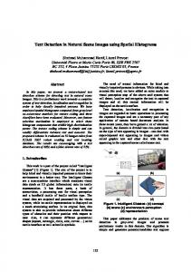
To train an over-complete dictionary for text signals using K-SVD algorithm, we need to first collect some data for training. It would be extremely tedious to manually collect data from real scene images. Therefore, we use images of isolated machine-printed characters, which include 10 digits and lowercase and uppercase letters. There are 12 typefaces (such as Times New Roman, Arial, etc.) 4 styles (normal, bold, italic and bold italic) and 2 size variations (11 point and 8 point) in these images. Data were collected by the following procedure: 1. Generate the edge map for each character image using Canny operator. 2. Scan each edge map with a small window of size 16 × 16. If a long enough edge segment (with a length longer than 16) falls into the small scanning window, we generate a new observation by doing the following: initialize with zero a new image of the same size as the scanning window; center the edge segment into this image; convert this image to a vector by concatenating its rows. 3. The newly generated observation is added into the observation set if it is significantly different from other observations already in the set. The difference between observations is measured by Euclidean distance between vectors. In total, we have collected 12278 observations from the edge maps of these isolated character images. On the left of Fig.1, we give some examples of the observations we used for dictionary learning. It would be tempting to use the whole character edge map as one observation. This idea does not work well because it usually results in long observation vectors and would take the K-SVD too much time to learn. Therefore, instead of working on the whole edge map, we only look at the curve segments on the edge of characters. We also need to pay attention to the size of the sliding window. If it is too large, again it will generate very long observation vectors and thus increase the difficulty in learning. If it is too small, the curve segments would not bear too much character shape information and therefore become not so useful in text detection. In
we solve for x in the following equation using OMP: y = Dx
Figure 1. Left: Examples of the observations taken from character edges for learning the dictionary. Right: The most frequently used atoms learned by K-SVD.
our experiments, we found that 16×16 is the best tradeoff. Another important point is that we need to center the edge segment in the newly generated image. This is because the learned dictionary D is not shift-invariant: it will give quite different representations to shifted versions of the same observation. Therefore, in both data collecting and text detection, we explicitly center the edge segment at the center of the small image patch. In applying the K-SVD algorithm, there are two important parameters we need to choose: the redundancy factor Rf and the number of elements in each linear combination, or T0 . These values are chosen empirically so that good text detection performance can be achieved. Details of the parameter selection process will be discussed in the experimental results section.
3
Text Detection via Sparse Representation
When an image is given, we first extract the edges using Canny edge detector and then group these edge points into connected components (CC). CCs correspond to long lines are removed.
3.1
Connected Components Labeling
The labeling procedure actually consists of two stages: pixel level labeling and connected component level labeling. At the pixel level labeling, the edge map is scanned using a 16 × 16 window in a similar way as we scan the character edge map in data collecting. The scanning step is set to 4 pixels in both directions. If a long enough edge segment (with a length longer than 16) falls into the small window, we generate an observation vector y as we have done in data collecting and
(5)
Here D is the over-complete dictionary we have learned. If x is sparse enough , we label pixels on this edge segment as text. By saying sparse enough, we mean that x has at most T1 = 16 non-zero components. This number is empirically chosen based on a dataset of 120 real scene images. The results of this pixel level labeling on three sample images are shown in Fig.2. At connected component level labeling, we label each connected component as text if more than 25 percent of its points have been labeled as text at pixel labeling stage. Here we intentionally choose a low threshold to avoid missing true text components.
3.2
Layout Analysis
After the labeling procedure, we apply layout analysis to filter out some of the possible false detections. We merge horizontally neighboring CCs with similar size into a structure called “Line”. After this line growing procedure, we will discard those short LINEs (with fewer than 3 CCs) unless they have more than 80 percent of the edge points been labeled as text at pixel level labeling stage. The detected text LINEs are shown in Fig.2. In these examples, we draw the bounding box of each LINE together with the bounding boxes of the connected components inside that LINE.
4
Experimental Results
A database of 120 scene images has been collected to help us in selecting the parameters used in the proposed method. To evaluate the proposed method, we use the 2003 ICDAR (International Conference on Document Analysis and Recognition) Text Location Contest trial test database, which is publicly available and can be downloaded at http://algoval.essex.ac.uk/icdar/Datasets.html. Included in this database are 251 images and the ground truth of the word bounding boxes of all the target texts in these images. The evaluation is based on the notions of precision and recall. Precision, p, is defined as the number of correct word detection divided by the total number of detection. Recall, r, is defined as the number of correct word detection divided by the total number of the word in the ground truth. As mentioned above, we have experimentally selected two main parameters in the K-SVD algorithm:
(a) Example A. (a)
(b) Example B.
(b)
Figure 3. (a) Recall rate of the proposed algorithm under different parameter settings. (b) Precision of the proposed algorithm under different parameter settings.
(c) Example C.
Figure 2. Some examples generated by the proposed method. In each example, the top left gives the input grayscale image; the top right gives edge map generated by Canny operator; the bottom left gives the pixel level labeling results; the bottom right gives the text LINEs detected after layout analysis.
the redundant factor Rf and the sparse threshold T0 . Let Rf ∈ {1, 2, 3, 4, 5} and T0 ∈ {6, 7, 8, 9, 10}. We have exhaustively tried all combinations of these two parameters on the training dataset and the performance of these experiments are shown in Fig3. From these experiments, we can see that as the redundant factor Rf grows, the recall rate also grows. However, the difference between Rf = 4 and Rf = 5 is not significant. If we fix the parameter Rf and let T0 grow, the recall rate also increases, since more edge points can be labeled as text. The situation is different when it comes to the precision of text detection. When Rf starts to grow, the precision grows too, but very slowly. While Rf grows to 5, the precision even
Method [8] [5] Proposed method
p(precision) 56.3% 55.8% 67.64%
r(recall) 64.3% 68.9% 75.23%
Table 1. Experimental results and comparison.
starts to fall. For each fixed Rf , the precision gradually starts to fall while T0 grows. As the tradeoff between recall rate and detection precision, we choose T0 = 8 and Rf = 4, which means we have 1024 atoms in the dictionary. On the right of Fig.1, we give some of the most frequently used learned atoms when reconstructing the observations. Even though many text detection methods can be found in the literature, most of them report results on private databases. To the best of our understanding, only two methods [8, 5] have reported their results on the public database adopted in this paper. In [8], three algorithms have been investigated. The first method is composed of gray value stretching and binarization by an average intensity of the image. The second method is a Split and Merge approach which is one of the wellknown algorithms for image segmentation. The third one is a combination of the two methods. In the following comparison, results of the third method are reported. In [5], low-level image features and high-level text stroke features are combined hierarchically and SVM is applied for final verifications. We include these results together with ours in Table 1.
5
Conclusion
In this paper, a text detection method based on sparse representation is proposed. This idea is inspired by the result from vision research. Experimental results show that such a mechanism could be an interesting computation model for text detection in images. It is also possible to apply this model to other object detection problems. Our future research also involves applying this idea to pattern recognition problems, such as handwritten numeral recognition.
References [1] M. Aharon, M. Elad, and A. Bruckstein. The k-svd: An algorithm for designing of overcomplete dictionaries for sparse representation. IEEE Trans. Signal Processing, 54(11):4311–4322, 2006.
[2] D. Chen and J. Luettin. A survey of text detection and recognition in images and videos. RR-00-38, IDIAP, 2000. [3] X. Chen, J. Yang, J. Zhang, and A. Waibel. Automatic detection and recognition of signs from natural scenes. IEEE Transactions on Image Processing, 13(1):87–99, 2004. [4] X. Chen and A. L. Yuille. Detecting and reading text in natural scenes. In Proc. IEEE Conference on Computer Vision and Pattern Recognition, 2004. [5] Y. Choi. Scene text extraction in natural images using hierarchical feature combining and verification. In the 2nd KAIST-Tsinghua Joint Workshop on Pattern Recognition, pages 76–102, 2003. [6] J. Gao and J. Yang. An adaptive algorithm for text detection from natural scenes. In Proceedings of IEEE Computer Society Conference on Computer Vision and Pattern Recognition, volume II, pages 84–89, 2001. [7] K. Jung, K. I. Kim, and A. K. Jain. Text information extraction in images and video: a survey. Pattern Recognition, 37:977–997, 2004. [8] J. Kim, S. Park, and S. Kim. Text locating from natural scene images using image intensities. In Proceedings of eighth International Conference on Document Analysis and Recognition, volume 2, pages 655–659, 2005. [9] B. Olshausen and D. Field. Sparse coding with an overcomplete basis set: a strategy employed by v1? Vision Research, 37:3311–3325, 1997. [10] J. A. Tropp. Greed is good: Algorithmic results for sparse approximation. IEEE Trans. Inf. Theory, 50(10):2231–2242, 2004.