Astronomical relativistic reference systems with multipolar ... - CiteSeerX

RAA 2014 Vol. 14 No. 9, 1193–1200 doi: 10.1088/1674–4527/14/9/009 http://www.raa-journal.org http://www.iop.org/journals/raa

Research in Astronomy and Astrophysics

Astronomical relativistic reference systems with multipolar expansion: the global one ∗ Yi Xie School of Astronomy & Space Science, Nanjing University, Nanjing 210093, China; [email protected] Key Laboratory of Modern Astronomy and Astrophysics, Nanjing University, Ministry of Education, Nanjing 210093, China Received 2013 October 10; accepted 2014 March 6

Abstract With the rapid development of techniques for astronomical observations, the precision of measurements has been significantly increasing. Theories describing astronomical relativistic reference systems, which are the foundation for processing and interpreting these data now and in the future, may require extensions to satisfy the needs of these trends. Besides building a framework compatible with alternative theories of gravity and the pursuit of higher order post-Newtonian approximation, it will also be necessary to make the first order post-Newtonian multipole moments of celestial bodies be explicitly expressed in the astronomical relativistic reference systems. This will bring some convenience into modeling the observations and experiments and make it easier to distinguish different contributions in measurements. As a first step, the global solar system reference system is expressed as a multipolar expansion and the post-Newtonian mass and spin moments are shown explicitly in the metric which describes the coordinates of the system. The full expression of the global metric is given. Key words: reference systems — gravitation 1 INTRODUCTION Recent years have witnessed the rapid development of techniques for astronomical observations, causing the precision of measurements to significantly increase. One example is the space astrometry mission Gaia, which was launched by the European Space Agency (ESA) in 2013 (see Lindegren et al. 2008; Lindegren 2010, for recent reviews). It will obtain accurate astrometric data for ∼ 109 objects from 6th to 20th magnitude. The accuracies for single stars down to 15th magnitude typically range from 8 to 25 microarcseconds (µas). With such a high performance, Gaia will be able to detect the relative positional change of a star due to the first order post-Newtonian (1PN) effects from the spherically symmetric parts of gravitational fields of the Sun and some giant planets (Klioner 2003). In some cases where the observed source is very close to the surfaces of Jupiter and Saturn, the higher order multipole moments might cause 1PN light bending up to the level from several tens to hundreds of µas (Klioner 1991; Kopeikin 1997; Klioner 2003), which are also observable by Gaia. ∗ Supported by the National Natural Science Foundation of China.

1194

Y. Xie

Future space missions may even go further by measuring distances of laser links and angles among these links with unprecedented precision, such as the T´el´emetrie InterPlan´etaire Optique (TIPO) (Samain 2002), the Laser Astrometric Test Of Relativity (LATOR) (Turyshev et al. 2004), the Astrodynamical Space Test of Relativity using Optical Devices (ASTROD) (Ni 2008), the Search for Anomalous Gravitation using Atomic Sensors (SAGAS) (Wolf et al. 2009), the Phobos Laser Ranging (PLR) (Turyshev et al. 2010) and the Beyond Einstein Advanced Coherent Optical Network (BEACON) (Turyshev et al. 2009). Some of them might be able to measure not only 1PN effects caused by the quadrupole moment of the Sun but also effects of the second order post-Newtonian (2PN) light deflection resulting from intrinsic nonlinearity of gravity with high precision. On the surface of the Earth, time keeping and dissemination equipment are also undergoing great improvements such as optical clocks (e.g. Chou et al. 2010) and optical fiber networks (e.g. Predehl et al. 2012). These technologies will be able to measure the Earth’s gravitational potential to new levels of precision by gravitational time dilation at the scale of daily life (Chou et al. 2010) and might bring some subtle effects due to the multipole moments of the Earth into their thresholds in the not-so-distant future. Although, for processing and interpreting these data now and in the future, the International Astronomical Union (IAU) 2000 and subsequent Resolutions1 on reference systems in the solar system for astrometry, celestial mechanics and metrology in the framework of general relativity (GR) (Soffel et al. 2003) provide a solid foundation, extensions might be required in some specific observations and measurements. To model the light propagation in those observations and experiments accessing 2PN GR effects, some efforts are dedicated to making the IAU Resolutions include all these contributions (e.g. Minazzoli & Chauvineau 2009). Meanwhile, some works are devoted to establishing self-consistent astronomical relativistic reference systems compatible with alternative relativistic theories of gravity, such as the scalar-tensor theory (Kopeikin & Vlasov 2004), setting up a framework for testing GR. Under these systems, the 2PN theory of light propagation is studied in astronomical observations and experiments using large bodies in the solar system (e.g. Minazzoli & Chauvineau 2011; Deng & Xie 2012). Astronomical relativistic reference systems for gravitational subsystems are also introduced for the advanced theory of lunar motion and for a new generation of lunar laser ranging (Kopeikin & Xie 2010; Xie & Kopeikin 2010). When higher order post-Newtonian approximation for light propagation is considered, it will also be necessary to ensure the 1PN multipole moments of celestial bodies are explicitly expressed in the astronomical relativistic reference systems. Because, in some cases like the LATOR mission, the light bending caused by the quadrupole at 1PN order can be comparable with those due to the monopole at 2PN order (Klioner 2003). It also helps to distinguish effects from the 1PN multipole moments as well as the intrinsic nonlinearity of gravity at 2PN order. However, the IAU Resolutions on astronomical relativistic reference systems are written in the forms of integrals without showing explicit dependence on the mass and spin multipole moments of each local gravitating body, which may cause some inconvenience in modeling the observations, experiments and data analysis. To achieve this purpose, it is necessary to apply the techniques of multipolar expansion of the gravitational field, which have been intensively studied by many researchers (e.g. Sachs 1961; Pirani 1965; Bonnor & Rotenberg 1966; Epstein & Wagoner 1975; Wagoner 1979; Thorne 1980; Blanchet & Damour 1986; Blanchet 1987; Tao & Huang 1998). Thus, in this work, I will focus on astronomical relativistic reference systems with multipolar expansion. More specifically, this approach ensures the 1PN multipole moments are expressed explicitly in the mathematical description of the reference systems within the framework of the scalartensor theory. As a first step, only the solar system barycentric reference system — the global one — will be considered here. Local reference systems with multipolar expansion will be presented in subsequent works. 1

Resolutions adopted at the IAU General Assemblies: http://www.iau.org/administration/resolutions/general assemblies/

Global Reference System in a Multipolar Expansion

1195

The rest of the paper is organized as follows. Section 2 is devoted to debriefing primary concepts in astronomical relativistic reference systems. In Section 3, I present the outline of the techniques of multipolar expansion for astronomical relativistic reference systems (a demonstration is given in Appendix B, see online version). The full mathematical description of the solar system barycentric reference system with multipolar expansion and its two special cases are shown in Appendix C (see online version). Finally, in Section 4, I summarize the results. 2 BASICS OF ASTRONOMICAL RELATIVISTIC REFERENCE SYSTEMS Theories of astronomical relativistic reference systems have been intensively studied (e.g. Kopejkin 1988; Brumberg & Kopejkin 1989; Brumberg 1991; Damour et al. 1991, 1992, 1993; Klioner 1993; Klioner & Voinov 1993; Klioner & Soffel 1998; Kopeikin & Vlasov 2004; Kopeikin & Xie 2010; Xie & Kopeikin 2010). The following part of this section will only give an overview of the primary concepts and necessary mathematical description (see Kopeikin et al. 2011; Soffel & Langhans 2013, for recent reviews and more details). A reference system is a mathematical construction which gives “names” to spacetime events and a reference frame is a realization of the reference system. A well-defined reference system is the solid and robust foundation for a reference frame which can be materialized by astronomical catalogs and/or dynamical ephemerides of celestial bodies. One leading purpose of classical astrometry in the Newtonian framework is to establish an inertial celestial reference frame. However, this Newtonian concept of absolute space and time is abandoned in GR. In the 4-dimensional curved spacetime, time and space are two parts of a single event. The curvature of spacetime determines motion of matter and the matter, in turn, affects geometry of the spacetime. An astronomical relativistic reference system is a mathematical description which assigns coordinates (four real numbers) xµ (µ = 0, 1, 2, 3) for an event within it. Among four coordinates, x0 is the time coordinate: t = c−1 x0 is the coordinate time where c is the speed of light; and the remaining three xi (i = 1, 2, 3) are space coordinates. The coordinates xα = (ct, xi ) as a whole are described by the metric tensor gµν (xα ) which is a solution of the field equations of Einstein’s GR or other alternative relativistic theories of gravity. The metric tensors of reference systems and the coordinate transformations between them hold all of the properties of the reference systems. Although all reference systems are mathematically equivalent, using some specific systems can largely simplify calculations in modeling astronomical and astrophysical processes. In the solar system, an adequate relativistic description of a gravitational body’s motion is not conceivable without a self-consistent theory of astronomical relativistic reference systems, because the solar system has a hierarchical structure with a diversity in various masses of the bodies and the presence of planetary satellite systems which form a set of gravitationally bounded subsystems. The Sun is the most massive body in the system, but giant planets, like Jupiter and Saturn, can still make it revolve at some distance around the solar system barycenter (SSB). Thus, a global solar system barycentric reference system is required to describe the orbital motion of bodies in the solar system and model the light propagation from distant celestial objects. On the other hand, rotational motion of a body is more natural for describing the local reference systems associated with each of the bodies. A local reference system of a body is also adequate for describing its figure and satellites’ motion. Sometimes, a planet may have natural satellites with non-negligible masses which form a gravitational subsystem. It is convenient to introduce a local reference system associated with the barycenter of the subsystem, which leads to a natural decomposition of orbital motion of the subsystem around SSB and relative motion inside the subsystem. In 2000, IAU adopted new resolutions which laid down a self-consistent general relativistic foundation for applications in modern geodesy, fundamental astrometry, celestial mechanics and spacetime navigation in the solar system. These resolutions combine two independent approaches to the theory of relativistic reference systems including the global one and local ones in the solar

1196

Y. Xie

system developed in a series of publications by Brumberg and Kopeikin (BK formalism) (Kopejkin 1988; Brumberg & Kopejkin 1989; Brumberg 1991) and Damour, Soffel and Xu (DSX formalism) (Damour et al. 1991, 1992, 1993, 1994). To make the IAU Resolutions fully compatible with modern ephemerides of the solar system (e.g. Pitjeva 2005; Folkner 2010; Fienga et al. 2011) which employ the generalized Einstein-InfeldHoffman (EIH) equations (Einstein et al. 1938) with two parameterized post-Newtonian (PPN) parameters β and γ, some efforts (Klioner & Soffel 2000; Kopeikin & Vlasov 2004) have been contributed. They can go back to the IAU Resolutions when β = 1 and γ = 1. I will follow the approach of Kopeikin & Vlasov (2004) in this work. The metric tensor gµν (xα ) under 1PN approximation for any reference system can be formally written as g00 = −1 + ²2 N + ²4 L + O(²5 ) ,

(1)

g0i = ²3 Li + O(²5 ) ,

(2)

gij = δij + ²2 Hij + O(²4 ) ,

(3)

where ² ≡ 1/c and N , L, Li and Hij are coefficients of the metric. These coefficients can be solved from the field equations of Einstein’s GR or other alternative relativistic theories of gravity with certain boundary conditions. In particular, to solve the metric tensor for the solar system barycentric reference system, it is assumed that the solar system is isolated and there are no masses outside it. The considered number of bodies in the system depends on the required accuracy. Therefore, the spacetime of the solar system is asymptotically flat at infinity with the metric tensor gµν approaching the Minkowskian metric ηµν = diag(−1, +1, +1, +1). In addition, “no-incoming-radiation” conditions are also imposed on the metric tensor to prevent the appearance of non-physical solutions (see Kopeikin & Vlasov 2004, for details). Its coordinates xα cover the entire spacetime of the solar system and their origin coincides with the SSB at any instant of time. The law of conservation of angular momentum in the solar system can make the spatial axes of the global coordinates non-rotating in space either kinematically or dynamically (Brumberg & Kopejkin 1989). A reference system is called kinematically non-rotating if its spatial orientation does not change with respect to the Minkowskian spacetime at infinity as time goes on. A dynamically non-rotating system is defined by the condition that equations of motion of test particles moving with respect to the system do not have any terms that can be interpreted as the Coriolis or centripetal forces. With these assumptions and conditions, the metric tensor gµν (xα ) can be obtained in the 1PN approximation within the framework of the scalar-tensor theory (Kopeikin & Vlasov 2004) and the solutions of its coefficients are given in Appendix A (see online version) in the form of integrals. Theoretically, this metric can be taken to model observations and experiments; however, its dependence on integrals makes this expression inconvenient and non-intuitive in practice. Thus, in the next section, these integrals will be multipolarly expanded and expressed in terms of local mass and spin multipole moments of each bodies. This would make the metric tensor easier to deal with and show the physical contribution of multipole moments more clearly. 3 MULTIPOLAR EXPANSION OF GLOBAL REFERENCE SYSTEM To realize the purpose of this work, I need to apply the techniques of relativistic multipolar expansion of the gravitational field, which involves some parameters of the so-called mulitpole moments. In the Newtonian framework, multipole moments are uniquely defined as coefficients in a Taylor expansion of the gravitational potential in powers of the radial distance from the origin of a reference system to a field point. They can be functions of time in the most general astronomical situations.

Global Reference System in a Multipolar Expansion

1197

Multipolar expansion in GR is quite different (see Thorne 1980, for a review). Because of the nonlinearity of the gravitational interaction, a proper definition of relativistic multipole moments is much more complicated. This issue has been intensively and widely studied (e.g. Sachs 1961; Pirani 1965; Bonnor & Rotenberg 1966; Epstein & Wagoner 1975; Wagoner 1979; Thorne 1980; Blanchet & Damour 1986; Blanchet 1987; Tao & Huang 1998). It was shown that, in GR, the multipolar expansion of the gravitational field of an isolated gravitating system is characterized by only two independent sets: mass-type and current-type multipole moments (Thorne 1980; Blanchet & Damour 1986; Blanchet 1987). In the scalar-tensor theory of gravity, the multipolar expansion becomes even more complicated due to the scalar field. It introduces an additional set of multipole moments which are caused by the scalar field (see Kopeikin & Vlasov 2004, for details). In this work, I will follow and apply the techniques of multipolar expansion and definitions of multipole moments which have been studied in great detail and used in Kopeikin & Vlasov (2004). These required techniques are rather straightforward. All of the integrals in gµν (xα ) [see Eqs. (A.11)–(A.17) and (A.19)] for the global reference system can be written in the form (Kopeikin & Vlasov 2004) Z (C) In {f }(t, x) = f (t, x0 )|x − x0 |n d3 x0 , (4) VC

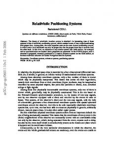
where n is an integer with values of either −1 or 1. It suggests that multipolar expansion of these integrals needs three steps: – Step 1. Taylor expand the integral (4) using the fact that the characteristic size of the body C is less than the characteristic distance between the field point, x, and the body C, xC , i.e. |x0 − xC | < RC , where RC = x − xC and RC = |RC |. Here xC represents the position of the center of mass of the body C with respect to the global system and it changes with the global time due to its orbital motion. See Figure 1 for the geometry of the vectors x, x0 , xC and RC . – Step 2. Convert the global coordinates x0 of a matter element inside body C into the local coordinates Z 0C with respect to the center of mass of body C: Z 0C = x0 − xC + O(²2 ) (see eq. (11.2.3) in Kopeikin & Vlasov 2004, for details). See Figure 1 for the geometry of the vector Z 0C . – Step 3. Collect and rearrange the expansion according to the definitions of mass and spin multipole moments (see eqs. (6.3.1) and (6.3.8) in Kopeikin & Vlasov 2004, for these definitions). To demonstrate this procedure, the multipolar expansion of UC (t, x) [see Eq. (A.11) is shown in Appendix B as an example.

Fig. 1 The geometry of the vectors x, x0 , xC , RC and Z 0C .

1198

Y. Xie

After applying it straightforwardly on all of the integrals, the global metric tensor gµν of the solar system barycentric reference system can be written as 2

(I ) (S) (F ) (B) 5 gµν = ηµν + h(I) µν + hµν + hµν + hµν + hµν + O(² ) ,

(5)

(I) (I 2 ) where hµν is the contribution from one-body interactions, hµν originates from two-body interac(S) (F ) (B) tions, hµν is due to spins, hµν contains scaling function AC and kinematic rotation FCkm , and hµν is (F ) caused by bad moments. Their full expressions can be found in Appendix C. hµν can be eliminated

by redefining mass multipole moments and by assuming local reference systems are kinematically (B) non-rotating (see Appendix C for details). It is worth mentioning that hµν is gauge-dependent so that it can be eliminated by a coordinate transformation of the time component as t0 = t + ²3 λ , where λ = 2(γ + 1)

µ ¶ ∞ XX 1 (−1)l (2l + 1) hLi GRC . (2l + 3)(l + 1)! RC ,hLi

(6) (7)

C l=0

hLi

Here, RC is a so-called “bad” moment defined in Equation (B.18) (Damour et al. 1992)2 . The 0 components of the new metric gµν are 0 gij = gij + O(²4 ) ,

(8)

0 g0i = g0i − ²3 λ,i + O(²5 ) ,

(9)

0 g00 = g00 − ²4 2λ,t + O(²5 ) .

(10)

The issue of coordinate transformations and gauges in the relativistic astronomical reference systems is practically important and it has been investigated in detail in several works (e.g. Tao & Huang 1998; Tao et al. 2000; Tao 2006). 4 CONCLUSIONS With advances in techniques for astronomical observations and experiments, the theories of astronomical relativistic reference systems might require extensions to satisfy the needs of new highprecision measurements. One direction is to ensure the 1PN multipole moments of celestial bodies are explicitly expressed in the reference systems. Since the effects of both these moments and nonlinearity of gravity are accessible for future space missions, it will bring some convenience for modeling the observations and experiments and make it easier to distinguish different contributions in measurements. Therefore, as a first step, the global solar system reference system is expressed as a multipolar expansion and the 1PN mass and spin moments are shown explicitly in their metric which describes the coordinates of the system. The full expression of the global metric is given (see Appendix C for details of main results). These results might be used in modeling future high-precision time transfer (e.g. Petit & Wolf 1994; Wolf & Petit 1995; Blanchet et al. 2001; Petit & Wolf 2005; Nelson 2011; Deng 2012; Deng & Xie 2013b,a; Pan & Xie 2013, 2014). Acknowledgements The work is supported by the National Natural Science Foundation of China (Grant No. 11103010), the Fundamental Research Program of Jiangsu Province of China (Grant No. BK2011553) and the Research Fund for the Doctoral Program of Higher Education of China (Grant No. 20110091120003). 2 Angle brackets surrounding a group of Roman indices denote the symmetric trace-free (STF) part of the corresponding three-dimensional object (see appendix A of Blanchet & Damour 1986, for details). Multi-index notations denote L ≡ i1 i2 · · · il and comma denotes a partial derivative. Therefore, Y,L = ∂ l Y /∂xi1 ∂xi2 · · · ∂xil .

Global Reference System in a Multipolar Expansion

1199

References Blanchet, L. 1987, Royal Society of London Proceedings Series A, 409, 383 Blanchet, L., & Damour, T. 1986, Royal Society of London Philosophical Transactions Series A, 320, 379 Blanchet, L., Salomon, C., Teyssandier, P., & Wolf, P. 2001, A&A, 370, 320 Bonnor, W. B., & Rotenberg, M. A. 1966, Royal Society of London Proceedings Series A, 289, 247 Brumberg, V. A. 1991, Essential Relativistic Celestial Mechanics (Bristol: Adam Hilger) Brumberg, V. A., & Kopejkin, S. M. 1989, Nuovo Cimento B Serie, 103, 63 Chou, C. W., Hume, D. B., Koelemeij, J. C. J., Wineland, D. J., & Rosenband, T. 2010, Phys. Rev. Lett., 104, 070802 Chou, C. W., Hume, D. B., Rosenband, T., & Wineland, D. J. 2010, Science, 329, 1630 Damour, T., Soffel, M., & Xu, C. 1991, Phys. Rev. D, 43, 3273 Damour, T., Soffel, M., & Xu, C. 1992, Phys. Rev. D, 45, 1017 Damour, T., Soffel, M., & Xu, C. 1993, Phys. Rev. D, 47, 3124 Damour, T., Soffel, M., & Xu, C. 1994, Phys. Rev. D, 49, 618 Deng, X.-M. 2012, RAA (Research in Astronomy and Astrophysics), 11, 703 Deng, X.-M., & Xie, Y. 2012, Phys. Rev. D, 86, 044007 Deng, X.-M., & Xie, Y. 2013a, RAA (Research in Astronomy and Astrophysics), 13, 1225 Deng, X.-M., & Xie, Y. 2013b, MNRAS, 431, 3236 Einstein, A., Infeld, L., & Hoffmann, B. 1938, Annals of Mathematics, 39, 65 Epstein, R., & Wagoner, R. V. 1975, ApJ, 197, 717 Fienga, A., Laskar, J., Kuchynka, P., et al. 2011, Celestial Mechanics and Dynamical Astronomy, 111, 363 Fock, V. A. 1959, The Theory of Space, Time and Gravitation (London: Pergamon Press) Folkner, W. M. 2010, in IAU Symposium, 261, eds. S. A. Klioner, P. K. Seidelmann, & M. H. Soffel, 155 Klioner, S. A. 1991, Soviet Ast., 35, 523 Klioner, S. A. 1993, A&A, 279, 273 Klioner, S. A. 2003, AJ, 125, 1580 Klioner, S. A., & Soffel, M. 1998, A&A, 334, 1123 Klioner, S. A., & Soffel, M. H. 2000, Phys. Rev. D, 62, 024019 Klioner, S. A., & Voinov, A. V. 1993, Phys. Rev. D, 48, 1451 Kopeikin, S., Efroimsky, M., & Kaplan, G. 2011, Relativistic Celestial Mechanics of the Solar System (Berlin: Wiley-VCH) Kopeikin, S., & Vlasov, I. 2004, Phys. Rep., 400, 209 Kopeikin, S., & Xie, Y. 2010, Celestial Mechanics and Dynamical Astronomy, 108, 245 Kopeikin, S. M. 1997, Journal of Mathematical Physics, 38, 2587 Kopejkin, S. M. 1988, Celestial Mechanics, 44, 87 Lindegren, L. 2010, in IAU Symposium, 261, eds. S. A. Klioner, P. K. Seidelmann, & M. H. Soffel, 296 Lindegren, L., Babusiaux, C., Bailer-Jones, C., et al. 2008, in IAU Symposium, 248, eds. W. J. Jin, I. Platais, & M. A. C. Perryman, 217 Minazzoli, O., & Chauvineau, B. 2009, Phys. Rev. D, 79, 084027 Minazzoli, O., & Chauvineau, B. 2011, Classical and Quantum Gravity, 28, 085010 Nelson, R. A. 2011, Metrologia, 48, 171 Ni, W.-T. 2008, International Journal of Modern Physics D, 17, 921 Pan, J.-Y., & Xie, Y. 2013, RAA (Research in Astronomy and Astrophysics), 13, 1358 Pan, J.-Y., & Xie, Y. 2014, RAA (Research in Astronomy and Astrophysics), 14, 233 Petit, G., & Wolf, P. 1994, A&A, 286, 971 Petit, G., & Wolf, P. 2005, Metrologia, 42, 138

1200

Y. Xie

Pirani, F. A. E. 1965, in Lectures on General Relativity, eds. S. Deser, & K. W. Ford, 249 (New Jersey: PrenticeHall, Inc.) Pitjeva, E. V. 2005, Astronomy Letters, 31, 340 Predehl, K., Grosche, G., Raupach, S. M. F., et al. 2012, Science, 336, 441 Sachs, R. 1961, Royal Society of London Proceedings Series A, 264, 309 Samain, E. 2002, in EGS General Assembly Conference Abstracts, 27, 5808 Soffel, M., Klioner, S. A., Petit, G., et al. 2003, AJ, 126, 2687 Soffel, M. H., & Langhans, R. 2013, Space-Time Reference Systems (Berlin: Springer) Tao, J.-H. 2006, Ap&SS, 302, 93 Tao, J.-H., & Huang, T.-Y. 1998, A&A, 333, 1100 Tao, J.-H., Huang, T.-Y., & Han, C.-H. 2000, A&A, 363, 335 Thorne, K. S. 1980, Reviews of Modern Physics, 52, 299 Turyshev, S. G., Farr, W., Folkner, W. M., et al. 2010, Experimental Astronomy, 28, 209 Turyshev, S. G., Shao, M., Girerd, A., & Lane, B. 2009, International Journal of Modern Physics D, 18, 1025 Turyshev, S. G., Shao, M., & Nordtvedt, K., Jr. 2004, Astronomische Nachrichten, 325, 267 Wagoner, R. V. 1979, Phys. Rev. D, 19, 2897 Will, C. M. 1993, Theory and Experiment in Gravitational Physics (Cambridge: Cambridge Univ. Press) Wolf, P., Bord´e, C. J., Clairon, A., et al. 2009, Experimental Astronomy, 23, 651 Wolf, P., & Petit, G. 1995, A&A, 304, 653 Xie, Y., & Kopeikin, S. 2010, Acta Physica Slovaca, 60, 393

Global Reference System in a Multipolar Expansion

A1

Appendix A: METRIC TENSOR FOR GLOBAL SOLAR SYSTEM BARYCENTRIC REFERENCE SYSTEM The metric tensor gµν (xα ) of the global solar system reference system can be solved in the 1PN approximation within the framework of the scalar-tensor theory as (Kopeikin & Vlasov 2004) g00 = −1 + ²2 N + ²4 L + O(²5 ) ,

(A.1)

g0i = ²3 Li + O(²5 ) ,

(A.2)

gij = δij + ²2 Hij + O(²4 ),

(A.3)

where ² ≡ c−1 and ϕ = U (t, x) ,

(A.4)

N = 2 U (t, x) ,

(A.5)

L = 2Ψ(t, x) − 2(β − 1)ϕ2 (t, x) − 2U 2 (t, x) −

∂ 2 χ(t, x) , ∂t2

Li = −2(1 + γ) Ui (t, x) ,

(A.6) (A.7)

Hij = 2γδij U (t, x) ,

(A.8)

in which x ≡ xi (i = 1, 2, 3) and ¶ µ 1 1 Ψ1 (t, x) − Ψ2 (t, x) + (1 + γ − 2β)Ψ3 (t, x) + Ψ4 (t, x) + γΨ5 (t, x) , (A.9) Ψ(t, x) ≡ γ + 2 6 Gravitational potentials U, U i , χ and Ψk (k = 1, ..., 5) can be represented as linear combinations of the gravitational potentials of each body in the gravitational system X X X X U= UC , Ui = UCi , Ψk = ΨCk , χ = χC , (A.10) C

C

C

C

where the summation index C numerates the bodies in the system, whose gravitational field contributes to the calculations. The gravitational potentials of the body C are defined as integrals taken only over the spatial volume VC of this body Z ρ∗ (t, x0 ) 3 0 d x, UC (t, x) = G (A.11) 0 VC |x − x | Z ρ∗ (t, x0 )v i (t, x0 ) 3 0 UCi (t, x) = G d x, (A.12) |x − x0 | VC Z ρ∗ (t, x0 )v 2 (t, x0 ) 3 0 ΨC1 (t, x) = G d x, (A.13) |x − x0 | V Z C ∗ ρ (t, x0 )h(t, x0 ) 3 0 ΨC2 (t, x) = G (A.14) d x, |x − x0 | V Z C ∗ ρ (t, x0 )ϕ(t, x0 ) 3 0 ΨC3 (t, x) = G d x, (A.15) |x − x0 | V Z C ∗ ρ (t, x0 )Π(t, x0 ) 3 0 ΨC4 (t, x) = G d x, (A.16) |x − x0 | VC

A2

Y. Xie

Z ΨC5 (t, x) = G VC

π kk (t, x0 ) 3 0 d x, |x − x0 |

(A.17)

where ρ∗ is the invariant density (Fock 1959), Π is the specific internal energy of matter, π αβ is the anisotropic tensor of stress, ϕ is the perturbation of the scalar field and h(t, x) = Hii (t, x). Potential χ is determined as a particular solution of the inhomogeneous equation ∇2 χ = −2U

(A.18)

with the right side defined over the whole space and it is Z χC (t, x) = −G ρ∗ (t, x0 )|x − x0 |d3 x0 .

(A.19)

VC

Mathematically, all of the integrals in Equations (A.11)–(A.17) and (A.19) can be written in the form (Kopeikin & Vlasov 2004) Z I(C) {f }(t, x) = f (t, x0 )|x − x0 |n d3 x0 , (A.20) n VC

where n is an integer with values of either −1 or 1. Appendix B: DEMONSTRATION OF MULTIPOLAR EXPANSION: THE CASE OF UC This section of the appendixes is devoted to demonstrating the procedure of multipolar expansion for the integrals in Equations (A.11)–(A.17) and (A.19). Since it is valid for each of them, we only take UC as an example and show the details of how to apply it. For other integrals, what is needed is just to repeat it. There are three steps. – Step 1. Taylor expand the integral (4) using the fact that the characteristic size of the body C is less than the characteristic distance between the field point, x, and the body C, xC , i.e. 0 0 RC < RC , where R0C = x0 − xC , RC = x − xC and RC = |R0C |, RC = |RC |. Here xC represents the position of the center of mass of the body C with respect to the global system. With the help of µ ¶ ∞ X 1 1 (−1)l 1 0hLi = = ∂L RC , (B.1) |x − x0 | |x − xC − (x0 − xC )| l! RC l=0

in which angle brackets surrounding a group of Roman indices denote the STF part of the corresponding three-dimensional object (see appendix A of Blanchet & Damour 1986, for details) and multi-index notations denote L ≡ i1 i2 · · · il and ∂L ≡ ∂i1 · · · ∂il , the integral in Equation (A.11) can be Taylor expanded as µ ¶ Z Z ∞ ρ∗ (t, x0 ) 3 0 X (−1)l 1 0hLi d x = ρ∗ 0 RC d3 x0 , (B.2) 0 l! RC ,L VC VC |x − x | l=0

where a comma denotes partial derivative. – Step 2. Convert the global coordinates x0 of a matter element inside the body C into the local coordinates Z 0C with respect to the center of mass of the body C. In the local reference system of the body C, the local coordinates of a field point in the vacuum are (cΞC , Z C ) and the coordinates of a matter element inside the body are (cΞC , Z 0C ), where ΞC is its local coordinate time, Z C is the position vector of the field point and Z 0C is the position

Global Reference System in a Multipolar Expansion

A3

vector pointing to the matter elements. These local coordinates have relationships with the global coordinates given as (Kopeikin & Vlasov 2004) 0 ΞC = t + ²2 ξC , i i 2 i ZC = RC + ² ξC , 0i 0i 0k k k ZC0i = RC + ²2 [ξC + VC0i (RC − RC )vC ],

(B.3) (B.4) (B.5)

i

i 0i i where RC = xi − xiC (t), RC = x0i − xiC (t), VC0i = v 0 − vC , 0 k k ξC = −(AC + vC RC ) + O(²2 ), µ ¶ 1 i k ijk j k i ik ik k ξC = v v + DC + FC RC + DC RC RC + O(²2 ), 2 C C µ ¶ 1 i k ijk 0j 0k 0i ik ik 0k ξC = v v + DC + FC RC + DC RC RC + O(²2 ), 2 C C

FCij = −εijk FCk , ¯C (xC ) − δ ik AC , Dij = +δ ik γ U C

ijk DC

1 = (ajC δ ik + akC δ ij − aiC δ jk ). 2

(B.6) (B.7) (B.8) (B.9) (B.10) (B.11)

Therefore, from Equations (B.5) and (B.8), it has ·µ ¶ ¸ 1 i k ijk 0j 0k 0i 0i 2 ik ik 0k RC = ZC − ² v v + DC + FC ZC + DC ZC ZC 2 C C k k 0k +²2 VC0i vC (RC − ZC ) + O(²4 ),

(B.12)

which will be a link connecting the global and local coordinates of a matter element. – Step 3. Collect and rearrange the expansion according to the definitions of mass and spin multipole moments. hLi According to Kopeikin & Vlasov (2004), the mass multipole moments IC are defined as · 2 Z Z ²2 d hLi 0hLi 3 0 0hLi 02 3 0 0 IC = σC (ΞC , Z C )ZC d ZC + σC (ΞC , Z 0C )ZC ZC d ZC 2(2l + 3) dΞ2C VC VC ¸ Z Z 2l + 1 d i 0 3 0 0 −4(1 + γ) σC (ΞC , Z 0C )ZC d ZC − ²2 d3 ZC σC (ΞC , Z 0C ) l + 1 dΞC VC VC · ½ ¸ ¾ ∞ X 1 0hLi K K 0K Q + 2(β − 1)PC ZC ZC , (B.13) × AC + (2β − γ − 1)PC + k! C k=1

in which σC (ΞC , Z 0C )

=

¶ ¸¾ ½ ·µ 1 0 0 0 2 2 V (Ξ, Z C ) + ΠC (ΞC , Z C ) − (2β − 1)UC (ΞC , Z C ) 1+² γ+ 2 C

ρ∗C (ΞC , Z 0C )

kk +²2 γπC (ΞC , Z 0C ),

(B.14) hLi

and the definitions of the spin moments SC are Z hLi 0L−1>p q 0 SC = εpq