Dynamic Pricing Strategies with Reference Effects - CiteSeerX

INFORMS

OPERATIONS RESEARCH Vol. 00, No. 0, Xxxxx 0000, pp. 000–000 issn 0030-364X | eissn 1526-5463 | 00 | 0000 | 0001

doi 10.1287/xxxx.0000.0000 c 0000 INFORMS °

Dynamic Pricing Strategies with Reference Effects Ioana Popescu INSEAD, Decision Sciences Area, Blvd. de Constance, 77300 Fontainebleau, France. [email protected], http://faculty.insead.edu/popescu/ioana

Yaozhong Wu INSEAD, Technology and Operations Management Area, Blvd. de Constance, 77300 Fontainebleau, France. [email protected]

We consider the dynamic pricing problem of a monopolist firm in a market with repeated interactions, where demand is sensitive to the firm’s pricing history. Consumers have memory and are prone to human decision making biases and cognitive limitations. As the firm manipulates prices, consumers form a reference price that adjusts as an anchoring standard based on price perceptions. Purchase decisions are made by assessing prices as discounts or surcharges relative to the reference price, in the spirit of prospect theory. We prove that optimal pricing policies induce a perception of monotonic prices, whereby consumers always perceive a discount, respectively surcharge, relative to their expectations. The effect is that of a skimming or penetration strategy. The firm’s optimal pricing path is monotonic on the long run, but not necessarily at the introductory stage. If consumers are loss averse, we show that optimal prices converge to a constant steady state price, characterized by a simple implicit equation; otherwise the optimal policy cycles. The range of steady states is wider the more loss averse consumers are. Steady state prices decrease with the strength of the reference effect, and with customers’ memory, all else equal. Offering lower prices to frequent customers may be suboptimal, however, if these are less sensitive to price changes than occasional buyers. If managers ignore such long term implications of their pricing strategy, the model indicates that they will systematically price too low and lose revenue. Our results hold under very general reference dependent demand models. Subject classifications : dynamic programming: deterministic; marketing: pricing, promotion, buyer behavior; inventory policies: marketing/pricing. Area of review : Manufacturing, Service and Supply Chain Operations History : Received February 2005; revised October 2005, January 2006; accepted February 2006

1. Introduction Traditional economic, marketing and operational models view the consumer as a rational agent who makes decisions based on current prices, income and market conditions. In a market with repeated interactions, such as frequently purchased consumer goods (e.g. gasoline), services (e.g. resort hotels, individual insurance) and B2B settings (e.g. media broadcasting, industrial maintenance), customers’ purchase decisions are also determined by past observed prices. As customers revisit the firm, they develop price expectations, or reference prices, which become 1

2

Popescu and Wu: Dynamic Pricing with Reference Effects c 0000 INFORMS Operations Research 00(0), pp. 000–000, °

the benchmark against which current prices are compared. Prices above the reference price appear to be “high”, whereas prices below the reference price are perceived as “low”. The latter effect stimulates short term demand and provides incentives for retailers to run price promotions as a mechanism to increase short-term profits. On the other hand, price promotions decrease consumers’ price expectations, and hence their willingness to buy the product at higher prices in the future. (We ignore stock-piling effects and assume that consumers are fully informed about product quality, and do not judge quality level by price.) For the firm, this means that high profits today may come at the expense of a loss in future demand, and hence less profit in the future. Therefore, a profit maximizing firm must consider the long term implications of its pricing strategy. Our goal is to characterize what types of pricing strategies are optimal in such repeated interaction markets. We investigate when the firm should use traditional skimming or penetration strategies, and whether a constant price versus a cycling policy is optimal in the long run. A distinctive feature of this work, compared to traditional microeconomic and operational frameworks, is that it relies on descriptive models of consumer behavior to derive pricing prescriptions under complex dynamics. Ultimately, we aim to provide normative insights on how behavioral demand parameters, such as customer loyalty and loss aversion, should reshape and reflect in managerial pricing decisions when customers have repetitive, long term relationships with the firm. The marketing literature provides compelling empirical evidence for the dependence of demand on past prices. Adaptation level theory (Helson 1964) predicts that customers respond to the current price of a product by comparing it to an internal standard formed based on past price exposures, called the reference price. While other reference price models exist in the literature, an empirical comparison conducted by Briesch et al. (1997) shows that “the best [...] model is [...] one that is based on the brand’s own price history”, i.e. an internal reference price mechanism. The impact of the reference price on demand, called reference effect, is behaviorally explained at the individual level by the postulates of prospect theory (Kahneman and Tversky 1979). Accordingly, consumers perceive prices as gains (discounts) or losses (surcharges) relatively to a reference price, and there is an inherent asymmetry in perception, in that losses loom larger than gains of the same magnitude (loss aversion). In addition, there is diminishing sensitivity to both gains and losses. The vast empirical validation of prospect theory in the context of reference prices is best synthesized by Kalyanaram and Winer (1995). Their “key empirical generalizations” validate the kinked S-shaped reference effect at the aggregate demand level. The value of this theory to managers and researchers alike is that “it predicts how consumers actually behave, rather than how they ought to behave” (Nagle and Holden 1995).


3

With few exceptions, the dynamic pricing literature is oblivious of such behavioral aspects underlying demand. Recent surveys on dynamic pricing confirm that the state of the art models unrealistically assume demand to be given exogenously, and customers’ purchase decisions to be based solely on the current price posted by the seller (Bitran and Caldentey 2003, Elmaghraby and Keskino¸cak 2003). Similarly, in industry practice, prices are typically based on empirically estimated demand models that reflect consumer response conditional on current prices only, indicating that firms typically follow myopic pricing policies. Recent research trends in dynamic pricing and revenue management investigate the issue of strategic buyer behavior, whereby consumers optimally time their purchase in anticipation of future prices (Ovchinnikov and Milner 2005, Liu and van Ryzin 2005). In parallel work, Heidhues and Köszegi (2005) propose an economic model where consumers’ stochastic reference points (for consumption and price) are determined as a rational expectation “personal” equilibrium. They investigate conditions for price stickiness in a static monopolistic framework with random cost. In contrast, we are interested in incorporating the impact of past prices on demand in a dynamic setting. Our consumers are more realistic than the traditional “homo economicus”, yet boundedly rational. They have memory and are prone to human decision making biases (such as anchoring effects and loss aversion) and cognitive limitations. In particular, they are unaware of their biases and do not act strategically. There are few demand models similar to ours in the dynamic pricing literature. Sorger (1988) studies local stability of joint dynamic pricing and advertising policies under reference price effects, but his results are not comparable to ours due to the compound advertising effect. Also, his Assumption 2 c. is inconsistent with our model. Kopalle et al. (1996) and Fibich et al. (2003) – henceforth KRA, respectively FGL – investigate a problem similar to ours under a much simpler linear demand model with (kinked) linear reference effects. KRA provide computational insights from a discrete time formulation (adapted from Greenleaf 1995), but their analytical results are limited. They conjecture and verify numerically (on p.66) the monotonic convergence of optimal prices under asymmetric demand effects; some special cases are proved in their Proposition 2. An elegant proof of this conjecture is due to FGL in a continuous time control framework. Their approach, contingent on a linear demand model, reduces the problem to solving a linear Euler equation. This cannot be solved explicitly for nonlinear models, hence “it is natural to ask whether the results of [their] study would remain valid for more general demand functions” (p.729), and precisely what general structural properties, if not


4

just linearity, drive these results. We extend their insights, and provide stronger analytical results, under very general modeling assumptions on demand. We provide structural, as opposed to parametric results, that allow to solve the monopolist’s dynamic pricing problem under a most general reference dependent demand model, that captures non-linearities and dynamics in response to changes in the reference price. The model is based on behavioral claims supported by empirical theories; it extends and generalizes existing models used in the literature (Sorger 1988, Greenleaf 1995, KRA, FGL). Our main technical contributions, detailed below, include a simple characterization of the steady state price, as well as convergence and monotonicity properties of the optimal pricing strategy. From a methodological standpoint, our approach suggests new ways of proving structural properties for dynamic programs with kinked rewards, which are the minimum of two smooth functions. We characterize the existence and uniqueness of an optimal constant pricing strategy on the long run (steady state). If consumers are loss seeking, i.e. more responsive to discounts than surcharges, the optimal policy cycles. If consumers are loss averse there is a range of steady states, reduced to a unique one in the loss neutral case. We provide a simple closed form characterization of the steady state, which allows for insightful sensitivity analysis with respect to behavioral parameters. The value of the steady state price decreases with customers’ loyalty (memory effects) and with their sensitivity to past prices (reference effects), all else equal. Also, the range of steady state prices is wider the more loss averse consumers are. If customers are heterogeneous in terms of their shopping frequency (and nothing else), retailers should offer discounts to loyal customers, and higher prices to occasional buyers (relatively to the unique price charged in a non-segmented market). While such strategies are consistent with current practices by retailers in consumer goods industries, our results indicate that they are not necessarily optimal if occasional buyers are more responsive to price changes than loyal ones. The steady state price is bounded between the profit maximizing price charged to consumers who don’t form reference effects, and the steady state price charged by a myopic firm to reference sensitive consumers. We show that firms who ignore the long term impact of reference price effects, will myopically but systematically underprice. Our results also characterize the transient monotonicity and convergence of price and reference price strategies. In general, we show that the strategic monopolist seeks a monotonic reference price strategy. If consumers’ reference price is initially high, they will be lead to perceive a gain in each period, as the firm will consistently price below the reference price. This perception of monotonic prices has the effect of a skimming strategy. Similarly, a low reference price leads to a penetration


5

type strategy. While high-low prices may be observed at the introductory stage, on the long run prices are eventually monotonic in the same direction as reference prices. We provide conditions for a monotonic pricing policy to be optimal (i.e. traditional skimming or penetration). This is true for example if consumers’ memory is short (i.e. the reference price equals the last price observed), or if reference prices have increasing marginal impact on demand. In particular, this includes the linear models studied by KRA and FGL. In summary, our results for general reference dependent demand models confirm the robustness of FGL and KRA insights concerning stability and steady state analysis, but not necessarily monotonicity of the transient pricing policy. The latter appears to be a result of their linear reference effect assumption. Our approach is similar in spirit to the two-stage method in FGL, but our analysis relies on structural arguments, as opposed to explicit solutions of a parametric model. The remaining of the paper is structured as follows. Section 2 describes a very general model of reference dependent demand based on behavioral findings, in particular prospect theory. We summarize behavioral claims that form the base of our various, parsimonious assumptions in the rest of the paper. Section 3 presents the dynamic pricing model. The next two sections are structured around consumer’s loss aversion. Section 4 focuses on models where consumers are loss neutral, with the loss seeking case briefly addressed at the end. We investigate the existence of the steady state, and stability and monotonicity properties of the optimal price and reference price strategies; these are benchmarked against myopic policies. Section 5 studies the same issues when consumers are loss averse, i.e. the reference effect is consistent with prospect theory. Section 6 concludes our findings.

2. General Reference Dependent Demand Model This section describes how consumers make purchase decisions based on prices and reference prices. The most prominent theory of reference dependent preferences is prospect theory (Kahneman and Tversky 1979); the deterministic versions in Thaler (1985) and Tversky and Kahneman (1991) are most relevant to our context. The mental accounting framework (Thaler 1985) proposes that the total utility from purchasing a product consists of two components: acquisition utility and transaction utility. The former corresponds to the monetary value of the deal, determined by the discrepancy between price and the value of the product to the consumer. Transaction utility corresponds to the psychological value of the deal, determined by the discrepancy between price and reference price. Thus, reference prices affect customer behavior via the magnitude of the perceived “gain” or “loss” x = r − p relative to


6

the reference point r. The microeconomic demand model induced by such individual preferences is derived by Putler (1992), who validates it empirically with egg sales data. Empirical validation of prospect theory at the demand level is remarkably synthesized by Kalyanaram and Winer (1995). Define the reference effect on demand R(r − p, r) = D(p, r) − D(p, p) as the differential demand at price p due to the reference price being r instead of the actual price p. Alternatively, R(x, r) measures the impact on demand of a perceived discount/surcharge x = r − p relative to the reference price r. Empirical evidence suggests that the larger magnitude of the perceived gain/loss, the larger the corresponding absolute impact on demand; this is known as Reference Dependence (RD). Furthermore, it has been observed that for normal goods purchase experience with higher past prices increases the likelihood of buying the product for a given observed price. This leads to the following standing assumption on the demand model: Assumption 1 (Reference Dependent Demand). Demand D(p, r) is non-negative bounded and continuous, decreasing in price p and increasing in the reference price r. The corresponding reference effect R(x, r) is increasing in x. In particular, the definition of the reference effect together with monotonicity of demand implies: Remark 1. R(x, r) ≥ 0 for x > 0, R(x, r) ≤ 0 for x < 0 and R(0, r) = 0. Furthermore, R(r − p, r) is increasing in r. We further describe the reference dependent demand model in terms of (1) how the perceived discount/surcharge x impacts demand and (2) how this impact varies with shifts in the reference value r. We provide behavioral claims, based on empirical generalizations and established theories of consumer behavior. These claims are the base of our parsimonious modeling assumptions in the rest of the paper. 2.1. Gain-Loss Asymmetries Behavioral theories suggest that consumers may react differently to discounts vs. surcharges. In particular, surcharges loom larger than discounts of the same magnitude (loss aversion). To measure these effects, we use the index of loss aversion ρ(r) =

λ− (r) , λ+ (r)

where λ− (r), λ+ (r) denote the left

and right x-derivatives of R(x, r) at x = 0 (Köbberling and Wakker 2005). People are loss averse at a given reference point r whenever ρ(r) exceeds 1. Asymmetries are considered robust, i.e. in a particular context consumers are unlikely to be loss averse for certain reference levels and loss seeking for others. This leads to the following alternative claims: Loss Aversion (LA): ρ(·) > 1; Loss Neutrality (LN): ρ ≡ 1; Loss Seeking (LS): ρ(·) < 1.


7

There is strong empirical evidence on loss aversion in the pricing context, with an observed index of loss aversion between 1.7-2.5 (see e.g. Ho and Zhang 2005, and references therein). In addition to reference dependence and loss aversion, prospect theory postulates that consumers exhibit diminishing sensitivity to both discounts and surcharges, leading to a kinked S-shaped reference effect. Diminishing Sensitivity (DS): R(x, r) is concave for x ≥ 0 and convex for x ≤ 0 for all r. Prospect Theory (PT): (RD), (LA) and (DS) hold for R(x, r). The pricing implications of prospect theory are further investigated in Section 5. Models with loss neutral and loss seeking buyers are investigated in Section 4. 2.2. Shifting Reference Price Limited work has been done to characterize dynamics of the reference effect when the status quo varies. A distinctive feature of our work is to incorporate such effects in the most general manner. Kahneman and Tversky (1979, p.277) suggest that the value function becomes more flat as the reference point increases. This is supported by empirical evidence from mental accounting studies (e.g. Thaler 1999). For example, many people would be happy to spend half an hour on the internet for a 50 Euro discount on a 100 Euro airplane ticket, but not on a 2000 Euro one. In both cases, however, costs (30 minutes) and benefits (50 Euro) are identical, so from a purely rational view point the trade-off is the same. This example indicates that consumers are less responsive to a given price change when the status quo price is higher. The following claim, adopted from the axiomatization of deference dependence by Schmidt (2003), captures this effect: Decreasing Curvature (DC): The marginal impact of a gain/loss x on demand decreases with the reference value r. Recall that a real-valued function f (x, y) is supermodular if it has increasing differences, i.e. f (x1 , y) − f (x2 , y) is increasing in y for all x1 > x2 . If f is differentiable, this amounts to positivity of the cross-partial derivative fxy (x, y) ≥ 0 (partial derivatives are denoted by corresponding subscripts). Submodularity is defined by the opposite inequality. Claim (DC) states that R(x, r) is submodular on the gain, respectively loss domain; this is irrespective of the gain-loss asymmetries discussed previously. An illustration of this claim under prospect theory is provided in Figure 1. 2.3. Absolute and Relative Difference Models. We next provide simple examples of reference effects used in the literature. The most common is the absolute difference (AD) model RAD (x, r) = h(x), with h increasing and h(0) = 0. The shape


8 Figure 1

Reference effect R(x, r) satisfying (P T ) and (DC).

1

0.5

R(x,r)

0

−0.5

−1

−1.5

−2 1 1.2 r 1.4 1.6 1.8 2

−1

−0.5

0.5

0

1

x

of the evaluation function h further controls for loss aversion, diminishing sensitivity etc. KRA and FGL use AD models with h (piecewise) linear. An important criticism to AD models is their failure to capture dynamics of the reference effect in response to changes in the reference price. A natural generalization that satisfies (DC) is R(x, r) = h(x)s(r), with s a positive decreasing scaling function. Another model used in the literature is the relative difference (RD) model RRD (x, r) = h( xr ) (with h increasing and h(0) = 0), motivated by the Weber-Fechner law in psychophysics. This law suggests that consumers perceive price differences in proportional, rather than absolute terms, a theory that is experimentally supported by mental accounting studies, such as the small example in the previous section (that can be explained by consumers not responding to the magnitude of the price differential r − p =50 Euro, but to the percentage difference relative to the base price: r−p r

= 50% vs. 4%). RD models have been used in conjunction with linear and logarithmic forms

for h (Winer 1988), as well as exponentials (Anderson and Rasmussen 2004). A generalization of RD models is R(x, r) = h(xs(r)), with s a positive decreasing scaling function. This satisfies (DC) if h is convex increasing, or h0 is inelastic to changes in x. While our analysis focuses on the most general reference dependence demand model, we systematically indicate how our general results specialize to the absolute and relative difference models.

3. Dynamic Pricing Model This section sets up our dynamic pricing model, together with general assumptions on how consumers’ memory works in adjusting reference prices based on price perceptions.


9

We consider a profit maximizing monopolist who faces a homogeneous stream of repeated customers over an infinite time horizon. The monopolist decides in every period what price p to charge to customers, from a bounded positive interval P = [0, p¯] (our results allow for a non-zero lower bound on price; see the Remark of Section B in the Appendix). The resulting profit is Π(p, r) = (p − c)D(p, r), where r is the current reference price and D(p, r) the corresponding demand satisfying Assumption 1. We assume for simplicity and without loss of generality the variable cost to be c = 0; all our results hold for a non-zero constant cost c. In each period, customers update their current reference price rt as they observe the new price pt charged by the firm. The adaptive expectation framework Nerlove (1958) motivates a reference price that is a weighted average of past prices, where more recent prices are given more weight. Throughout of the paper, we assume that the reference price formation mechanism is given by: rt = αrt−1 + (1 − α) pt−1 , α ∈ [0, 1).

(1)

Exponential smoothing is the most commonly used and empirically validated reference price mechanism in the literature (e.g. Winer 1986, Sorger 1988, Greenleaf 1995, KRA, FGL). Some of our results hold for more general mechanisms, including inflation effects and price trends in general (in this case our insights and results remain valid for inflation-adjusted prices). The memory model described by (1) allows for additional insights by quantifying the speed of the memory adjustment process. The memory parameter α captures how strongly the reference price depends on past prices. Lower values of α represent a shorter-term memory; in particular, if α = 0 then the reference price equals the past price. Memory is an indicator for shopping frequency, hence can be a proxy for customer loyalty. Actual estimated parameters range from α = 0 (Krishnamurthi et al. 1992) to α = 0.925 (Greenleaf 1995), much depending on the type of product or service involved. For an initial reference price r0 , we model the firm’s long term profit optimization problem as: V (r0 ) = sup

pt ∈P

s.t.

∞ X t=0

β t Π(pt , rt )

rt = αrt−1 + (1 − α)pt−1 ,

t ≥ 1,

where β ∈ (0, 1) is a discount factor. Profit-per-stage is bounded, so the value function is the unique bounded solution of the following Bellman equation (Stokey et al. 1989): V (r) = sup W (p, r), where W (p, r) = Π(p, r) + βV (αr + (1 − α)p).

(2)

p∈P

A consequence of Assumption 1 is that short term profit Π(p, r), and the value function are increasing (Stokey et al. 1989, Theorem 4.7), i.e. larger reference prices are preferable for the firm.


10

Remark 2. The value function V (r) is an increasing function of the reference price r. Because the action set P is compact and all functions are continuous, there exists an optimal stationary pricing policy that solves Problem (2), and associates with any given reference price r, one or more optimal prices. We define the optimal pricing policy as p∗ (r) = arg maxp W (p, r). To avoid the ambiguity of multiple solutions, arg maxx f (x) refers without loss of generality to the largest maximizer of the function f . The optimal reference price policy q ∗ (r) = αr + (1 − α)p∗ (r) provides the next reference price associated with the optimal pricing policy. The pricing path {p∗t } starting with an initial state r0 is computed sequentially as p∗t = p∗ (rt∗ ), where the state variable is updated in each period via the reference price formation mechanism ∗ rt∗ = q ∗ (rt−1 ). The sequence {rt∗ } of optimal reference prices is referred to as the state path; for

the consumer, this is the sequence of perceived prices or price expectations. A steady state p∗∗ for Problem (2) is one from which it is suboptimal to deviate, i.e. p∗ (p∗∗ ) = q ∗ (p∗∗ ) = p∗∗ , so the optimal price path starting at r0 = p∗∗ is constant. Our goal is to investigate when such a steady state exists and to characterize stability and monotonicity properties of the price and reference price paths. These results critically depend on consumer’s reaction to discounts and surcharges, captured by loss aversion.

4. Model without Loss Aversion This section focuses on the case when consumers are loss neutral (LN), i.e. the reference effect is smooth; loss seeking behavior is investigated at the end of this section. We first characterize the unique steady state, and then investigate stability and monotonicity properties of the price and reference price strategies, under very general modeling assumptions. Two additional assumptions are made throughout Sections 4.1-4.3. Assumption 2 (Smooth Reference Effect). R(x, r) is twice differentiable in x and r. The slope of the reference effect at x = 0 is denoted λ(r) = Rx (0, r). Our results require some typical technical assumptions on the short term profit Π(p, r) = π(p) + ΠR (p, r). Here π(p) = Π(p, p) = pD(p, p) is the profit in a market where consumers don’t form reference effects (R ≡ 0), referred to as base profit, and ΠR (p, r) = pR(r − p, r) is the profit from the reference effect, or reference profit. Assumption 3 (Profit). (a) π(p) is non-monotonic and concave in p. (b) Πp (r, r) = π 0 (r) − rλ(r) is strictly decreasing in r. (c) ΠR (p, r) is concave in p and supermodular in (p, r). Some intuition and motivation for these assumptions is provided next. Non-monotonicity of π(p) states that the firm is not constrained to charge sub-optimal prices (in a market without reference effects). This will allow to rule out pathological boundary steady states.


11

Part (b) states that, if the firm charges the reference price, a small change in price has higher impact on profit at lower reference prices. That is, marginal profit diminishes as price is set to the reference price. Strict monotonicity is necessary to insure uniqueness of the steady state. A sufficient condition for Assumption 3 (b), given (a), is rλ(r) strictly increasing in r. Diminishing marginal profit (concavity) is a typical economic assumption. Concavity of π and ΠR implies concavity of short term profit Π. The supermodularity (see p.7) assumption (c) states that marginal short term profit increases with the reference price. This is consistent with modeling assumptions used in the literature, and summarized by Winer (1988) (those demand functions are typically additively separable, in particular linear, in price and reference price). Various sets of sufficient conditions are provided in Section 5.3. One is supermodularity of demand D(p, r), which in particular implies that demand is more elastic at higher reference prices. In support of this assumption, Kamen and Toman (1970) found evidence that with higher reference prices, consumers were more likely to switch brands of gasoline, for a given price differential. 4.1. Myopic Strategies for Loss Neutral Buyers A firm that ignores the effect of current prices on future demand will focus on maximizing short term profit. Intuitively, such a myopic firm should charge higher prices as consumers’ price expectations are higher. This is insured by profit supermodularity (Assumption 3 (c)), via Topkis’ Theorem (Topkis 1998, Theorem 2.8.2 implies x∗ (y) = arg max f (x, y) increasing in y whenever f is supermodular). Lemma 1. The single period profit maximizing price p˜(r) = arg max Π(p, r) is increasing in r. p∈P

Formally, the problem solved by a myopic firm is equivalent to setting β = 0 (full discounting) in Problem (2). Consider two firms, one myopic, the other strategic (optimizer), starting with the same initial reference price r0 , and applying sequentially their respective pricing policies, while consumers’ memory evolves according to the same α-smoothing mechanism. The state of the system at time t, for the myopic and optimizing firms are given by rtM and rt∗ , respectively. The corre˜(rtM ) and p∗t = p∗ (rt∗ ). sponding myopic, respectively optimal prices charged at time t are pM t =p We show that the myopic firm systematically underprices, following a monotonic pricing strategy. The results are driven by supermodularity of short term profits (Assumption 3 (c)). Proposition 1 (Myopic vs. Strategic Firm). For any reference price r, the myopic firm underprices the product, i.e. p∗ (r) ≥ p˜(r). Furthermore, for any initial reference price r0 , the price ∗ charged by the myopic firm at any point in time is less than the optimal price, i.e. pM t ≤ pt , for all

t. Moreover, all myopic price paths monotonically converges to a unique constant price pM ∗ .


12

The prices charged by the myopic firm are oblivious of their eroding effect on future demand, hence future profits. By charging higher prices, the optimizing firm trades off current profits for future long-term profitability from higher reference prices. Figure 2 illustrates these results; in this case, the observed difference between optimal and myopic profits is about 10%. Throughout the paper, numerical examples are calculated using the Compecon Matlab toolbox developed by Miranda and Fackler (2002). Figure 2

Myopic vs. optimal pricing policies; D(p, r)= 1− 2p + r−p , P =[0.1, 0.3], α = 0.80, β = .95. 5r

Price

0.25

0.2

Optimal (r0=0.3) Myopic (r0=0.3) Optimal (r=0.1) Myopic (r0=0.1) 0.15

5

10

15

20 t

25

30

35

40

Figure 2 also suggests that the optimal pricing paths may converge monotonically to a single steady state price. These issues are investigated next. 4.2. Steady State for Loss Neutral Buyers Define the profit optimizing price in absence of reference effects p˜ = arg max π(p). The Bellman p∈P

equation (2) implies that, if a steady state p∗∗

π(p∗∗ ) exists, then V (p∗∗ ) = , whereas generally 1−β

π(r) for all r ∈ P. Assumption 3 (a,b) insures that such a steady state is unique and can 1−β be computed as the solution of a simple implicit equation: V (r) ≥

Theorem 1 (Steady State). If Problem (2) admits a steady state p∗∗ , then this is the unique solution of: π 0 (p) pλ(p) = . 1 − β 1 − αβ Furthermore, p∗∗ is continuously decreasing in α, increasing in β, and satisfies pM ∗ ≤ p∗∗ ≤ p˜.

(3)


13

At steady state, a small increase in price ∆p leads to a marginal increase in the long-term base profit equal to

π 0 (p) ∆p. 1−β

However, on the transition, customers perceive a loss and reduce their

demand. The resulting profit loss is pλ(p)∆p in the first period, αpλ(p)∆p in the second period and so on. Hence the implicit equation (3) reflects the balance between maximizing long-term profits (without reference effects) and the discounted transitory costs due to the reference effect. Equation (3) confirms that myopic firms (β = 0) set lower steady state prices pM ∗ . On the long run, strategic firms should charge lower prices when consumers form reference effects, than when they do not, i.e. p∗∗ ≤ p˜, approaching it as β → 1. In particular, Theorem 1 obtains the following closed form expressions for the corresponding steady states for absolute and relative difference models discussed in Section 2.3. This generalizes the FGL result for linear reference effects. Corollary 1 (Steady State for AD and RD Models). Consider the problem with linear base demand D(p, p) = b − ap, and reference effect RAD (x, r) = h(x), respectively RRD (x, r) = h(x/r). The corresponding steady states, if they exist, are p∗∗ AD =

b 2a+Λ

and respectively p∗∗ RD =

b−Λ , 2a

1−β where Λ = h0 (0) 1−αβ .

Consumer Heterogeneity and Sensitivity Analysis Insights. Consider a heterogeneous market, where consumer types differ in shopping frequency, captured by the memory parameter αi , and sensitivity to past prices, i.e. the reference effect Ri . Demands without reference effects are assumed identical across segments (i.e. Di (p, p) = D(p, p)). If the firm can segment the market, Theorem 1 indicates that on the long run, each segment should be charged a steady state price p∗∗ i that solves

π 0 (p) p(1−β)

=

λi (p) . 1−αi β

The steady state price only

depends on the reference effect via its slope at zero, specifically, it decreases with the magnitude of λ(·). That is, if consumers share the same memory parameter α, those who are more sensitive to past prices will be charged lower prices on the long run. Remark 3. If α1 = α2 and R2 is a “stronger” reference effect than R1 , i.e. if λ1 (r) ≤ λ2 (r) for all ∗∗ r, then the corresponding steady state prices, if they exist, satisfy p∗∗ 1 ≥ p2 .

On the other hand, if consumers only differ in their memory parameter αi , then segments with higher αi are charged lower steady state prices, all else equal. While charging lower prices to loyal customers (proxied by higher αi ) is in line with current practices in consumer goods industries, our results show that it may not be the optimal strategy if these shoppers are less sensitive to price changes, as measured by λi . In general, the firm should charge lower prices to segments with higher


14

long run marginal sensitivity to the reference effect, as measured by λi (·)/(1 − αi β). Specifically, ∗∗ the same argument as Remark 3 shows that p∗∗ 1 ≥ p2 , if

λ1 (r) 1−α1 β

≤

λ2 (r) 1−α2 β

holds for all r.

Finally, for comparison purposes, consider the case where the firm cannot segment the market and offers the same price to all segments. We show in Section D of the Appendix that the common steady PN λi (p) 0 (p) state price (if one exists) solves π1−β = p i=1 1−α , and is bounded between the lowest and highest iβ ∗∗ prices charged to each consumer type in a perfectly segmented market p∗∗ ∈ [mini p∗∗ i , maxi pi ].

4.3. Stability and Monotonicity with Loss Neutral Buyers This section investigates the existence and stability of the unique steady state price characterized in Theorem 1. We show global convergence of the optimal prices to steady state, and study local and global monotonicity properties of the state and optimal price paths. We start with the most general results that require no further assumptions. Recall that the reference price policy was defined by q ∗ (r) = αr + (1 − α)p∗ (r). Lemma 2 (Monotone Reference Price Policy).The reference price policy q ∗ (r) increases in r. The result follows from Assumption 3(c), and implies the following: Theorem 2 (Global Stability and State Path Monotonicity). Problem (2) admits a unique steady state p∗∗ , characterized by Theorem 1, to which all optimal price paths converge. All corresponding reference price paths converge to p∗∗ monotonically. Under the conditions of Theorem 2, the monopolist’s strategy involves decreasing customer’s price expectations by always pricing below the current reference price, or vice versa. If the reference price is high, the optimal pricing policy is a skimming-like strategy: the firm starts with a relatively high introduction price, then always prices below the reference price (rt > pt ). In this case, consumers perceive in each period a gain relative to their expectations, which stimulates demand, and hence profits in the current period. Low reference prices lead to a penetration-type strategy, whereby the firm always prices above the customers’ reference price (rt < pt ). The loss in current profit from a negative reference effect, is outweighed (1) by a higher short-term profit without reference effect, π(p∗t ), and (2) by the increase in future profits due to higher reference prices in the next period. Theorem 2 does not guarantee monotonicity of the corresponding pricing paths. This holds whenever the pricing policy is monotonic. Some sufficient conditions are provided next. Recall that a real-valued C 2 function f (x, y) is strongly concave if there exist positive constants a and b such that f (x, y) + ax2 + by 2 is concave.


15

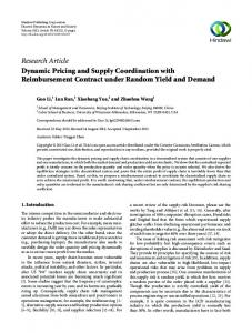
Lemma 3 (Monotone Price Policy). Each of the following alternative conditions is sufficient for the optimal pricing policy p∗ (r) in Problem (2) to be increasing in r : (a) Consumers have short memory α = 0, i.e. rt+1 = pt for all t; (b) Demand D(p, r), or equivalently, the reference effect R(r − p, r), is convex in r; (c) Short term profit Π(p, r) is strongly concave on the interior of its domain, and there exists a global constant K > 0 such that Πrr (p, r) ≥ −K and Πpr (p, r) ≥ K/2. The result follows from supermodularity of W (p, r), the function on the right hand side of the Bellman equation (2). This reduces to supermodularity of short term profit (Assumption 3 (c)) under condition (a). Condition (b) achieves this by additionally insuring convexity of short term profit in r, and hence of the value function. Condition (c) insures a uniform lower bound on the degree of concavity of the value function V, that is compensated by supermodularity of short term profits. At the limit, for K = 0 we recover the conditions of part (b). Strong concavity is a technical condition insuring second order differentiability of the value function. Theorem 3 (Global Price Monotonicity). Under the conditions of Lemma 3, all optimal pricing paths for Problem (2) converge monotonically to the unique steady state price p∗∗ , characterized by Theorem 1.

Figure 3

Optimal pricing paths for D(p, r) = e−p + 0.5(e0.5(r−p) − 1), α = 0.8, β = 0.9. 0.88

0.86

0.84

Price

0.82

0.8

0.78

0.76

0.74

5

10

15

20

25

30

t

In particular, we obtain the price monotonicity results of KRA and FGL for linear AD models RAD (x, r) = λx; these satisfy part (b) of Lemma 3. Part (c) of Lemma 3 (but not (b)) obtains price


16

monotonicity for linear RD models RRD (x, r) = λx/r, on a price range P = [p, p¯] with p¯/p ≤

√ 4 2,

i.e. price dispersion not exceeding 18%. Theorem 3 insures that only three possible pricing strategies are optimal: skimming (if initial price expectations are high, start with a high price and then keep decreasing it), penetration (if initial price expectations are low, start with a low price, then increase it), or constant pricing. Moreover, after a transient regime, the optimal prices stabilize to a steady state price. The results follow from the monotonicity of the policy function (Lemma 3). This also insures that the price paths do not cross, i.e. any increase in the initial reference price shifts the entire pricing sequence upwards. These results are illustrated with an example in Figure 3. Furthermore, in a neighborhood of the steady state, prices are eventually monotonic, i.e. local price monotonicity holds. Strong concavity of short term profits is a technical condition that insures differentiability of the value function and pricing policy. Proposition 2 (Local Price Monotonicity). If Π(p, r) is strongly concave on the interior of its domain, then all optimal pricing paths are locally monotonic around the steady state. Local price monotonicity implies that, on the long run, the slope of the reference price policy q ∗ (r) = αr + (1 − α)p∗ (r) is steeper than α. That is, reference prices converge to steady state at a rate that is ultimately faster than the memory parameter α. Transient High-Low Pricing. At the introductory stage, however, the monopolist may have an incentive to increase reference prices at a slower rate, achieved by high-low pricing. Such a strategy, depicted in Figure 4, contrasts the insights obtained by KRA and FGL under linear demand models. The optimal pricing policy p∗ (r) and price path {p∗t } are non-monotonic under the conditions of Theorem 2 and Proposition 2, but violating Lemma 3. The pricing strategy illustrated in Figure 4 is consistent for example with catastrophe insurance pricing in the U.S. before major hurricanes, when consumers reference prices are much lower than profit optimizing prices (we thank Paul Kleindorfer for suggesting this example; see endnote 1. for intuition). This example illustrates that high-low pricing is technically possible in the loss neutral case, contrary to previous insights in the literature; similar behavior can be observed for RD models. Nevertheless, extensive numerical simulations revealed that the optimal pricing path is typically monotonic; at most, it displays a relatively small direction swing from decreasing to increasing k

prices, as in Figure 4 (simulated models for R(x, r) include xe−ar , x/rk , 1 − e−ax , eax/r − 1, a, k > 0 for a variety of parameters satisfying Assumptions 1-3). So it is fair to say that, if consumers are loss neutral, we do not find strong numerical support for transient high-low pricing, but cannot rule it out either.


17 3

High-low pricing policy p∗ (r) and optimal price path p∗t ; D(p, p) = 2 − 0.5p, R(x, r) =0.5(e1.5x/r − 1),

Figure 4

P = [1, 2], α = 0.950, β = 0.999, r0 = 1. 2

2

1.99

1.99

1.98

1.98

1.97

1.97

1.96

Price

1.96 p*(r)

1.95

1.95 1.94

1.94 1.93

1.93 1.92

1.92

1.91

1.9

1

1.1

1.2

1.3

1.4

1.5 r

1.6

1.7

1.8

1.9

2

1.91

10

20

30

40

50 t

60

70

80

90

100

4.4. Loss Seeking Buyers High-low pricing is provably optimal if consumers are focused on gains, i.e. loss seeking (LS). In this case the optimal pricing policy for Problem (2) cycles. Consumers are loss seeking if they respond more to discounts than to surcharges, i.e. if the reference effect has a convex kink at zero. This type of asymmetry is inconsistent with prospect theory, but has found some empirical validation in the marketing literature (e.g. Krishnamurthi et al. 1992, Greenleaf 1995). We address it for completeness; only Assumption 1 stands in place for the next result: Proposition 3 (Cyclic Policy). If buyers are loss seeking, i.e. the reference effect R(x, r) satisfies (LS), then Problem (2) admits no steady state. Proposition 1 in KRA obtains a similar result when R(x, r) = h(x) is piecewise linear in x. Proposition 3 suggests that in order for a steady state price to exist, the reference effect R must be smooth, or kinked in the direction predicted by prospect theory. This case is analyzed next.

5. Model with Loss Aversion This section investigates the transient and long term behavior of the optimal dynamic pricing policy when reference effects are kinked in the spirit of prospect theory. We first set up the model; two additional assumptions on the reference effect, respectively profit are made throughout this section (replacing Assumptions 2 and 3 for the loss neutral case). 5.1. Model and Assumptions At the aggregate level, prospect theory predicts that the reference effect is captured by an S-shaped function of the reference gap x = r − p, with a concave (loss averse) kink at x = 0 (Kahneman and


18

Tversky 1979, Tversky and Kahneman 1991). The following assumption, made throughout this section, formalizes the technical aspects relevant for our purposes. An illustration is provided in Figure 5. Recall that a function f (x) is singlecrossing if there exists a unique x0 in its domain such that f (x0 ) = 0. We denote 1X the indicator function of the set X. Figure 5

An example of kinked reference effect RK

Assumption 4 (Kinked Reference Effect). The kinked reference effect is given by RK (x, r) = 1(x≥0) RG (x, r) + 1(x≤0) RL (x, r),

(4)

where RL (x, r) and RG (x, r) are twice differentiable, increasing in x with RG (x, r) − RL (x, r) singlecrossing in x, and satisfying λL (r) > λG (r) for all r. Assumption 4 is a weaker formalization of prospect theory (PT), as detailed in Section 2.1, including reference dependence (RD), and the weaker form of loss aversion (LA) in terms of the index ρ(r) =

λL (r) , λG (r)

proposed by Köbberling and Wakker (2005). We do not specifically assume

diminishing sensitivity (DS) (i.e. concavity/convexity of the gain/loss components), as it is immaterial for our analysis. The single crossing condition allows to write the kinked reference effect as the minimum of the loss and gain counterparts on the relevant domain: RK (x, r) = min(RG (x, r), RL (x, r)).

(5)


19

This condition is unrestrictive in the context of Assumption 4 alone, because the loss and gain parts of RK can always be smoothly extended so as to satisfy Eq. (5). Based on (5), the profit per-period can be written as ΠK (p, r) = min(ΠG (p, r), ΠL (p, r)),

(6)

where ΠG (p, r) = π(p) + pRG (r − p, r) and ΠL (p, r) = π(p) + pRL (r − p, r). In line with our previous assumptions on profit, the following technical assumption is made in this section: Assumption 5 (Gain/Loss Profit). The short term profits ΠG (p, r) and ΠL (p, r) associated with the smooth reference effects RG , respectively RL , satisfy Assumption 3. Section 5.3 provides sufficient modeling conditions on the reference effect for Assumptions 4 and 5 to hold, in particular when RK is convex-concave, as predicted by prospect theory. In particular, it provides concrete ways to construct RL , RG that satisfy Assumption 3, and so that Eq. (5) holds. The corresponding Bellman equation for the problem with kinked demand effect is: (K)

VK (r) = sup{ΠK (r, p) + βVK (αr + (1 − α)p)}.

(7)

p

5.2. Steady State, Stability and Monotonicity We extend the results obtained in Section 4 for the loss neutral case, to infer existence and stability properties of the steady state for loss averse buyers. A key role in our analysis here is played by the problem with smooth reference effect: Rθ (x, r) = θRG (x, r) + (1 − θ)RL (x, r).

(8)

Denoting the corresponding short term profit Πθ (p, r) = π(p) + pRθ (r − p, r), this problem is (Pθ )

Vθ (r) = sup{Πθ (p, r) + βVθ (αr + (1 − α)p)}.

(9)

p

For any θ ∈ [0, 1], Problem (Pθ ) satisfies our assumptions for the loss neutral case, so all the results of Section 4 apply. Moreover, Eq. (5) implies RK (x, r) = min(RG (x, r), RL (x, r)) ≤ Rθ (x, r), θ ∈ [0, 1].

(10)

The same relationship between short term profits, and the corresponding value functions is implied. The proof details of the following result are in the Appendix: Lemma 4. For any θ ∈ [0, 1], Problem (Pθ ) satisfies Assumptions 1-3. Its value function satisfies Vθ (r) ≥ VK (r) for all r, and its steady state p∗∗ θ is also a steady state for Problem (K).


20

By loss aversion and construction (8), the slopes of the reference effects RL , Rθ and RG satisfy λL (r) ≥ λθ (r) ≥ λG (r). Remark 3 further implies that the steady state prices of the corresponding ∗∗ ∗∗ ∗∗ problems satisfy p∗∗ L ≤ pθ ≤ pG . Moreover, as θ ∈ [0, 1], the steady states pθ span the interval ∗∗ [p∗∗ L , pG ].

We are now ready to characterize the set of steady states for general non-linear loss-averse demand effects, and their stability properties, as follows: Theorem 4 (Steady State, Stability and Monotonicity under Loss Aversion). The set ∗∗ ∗∗ ∗∗ of steady states for Problem (K) equals [p∗∗ L , pG ], so for an initial reference price r0 ∈ [pL , pG ], the ∗ optimal price path is constant p∗t = r0 . For an initial reference price r0 < p∗∗ L , respectively r0 > pG , ∗∗ the reference price path {rt∗ } converges monotonically to p∗∗ L , respectively pG , and the corresponding

optimal price path {p∗t } also converges to the same steady state. Our analysis, based on bounding the kinked reference effect, and hence corresponding value function, by the full range of convex combinations of the smooth loss and gain counterparts, suggests a general approach for obtaining structural properties and global stability in dynamic programs with kinked reward structure. A similar approach is used by FGL in their analysis of kinked linear demand models; their results are driven by the explicit solution of the linear demand model, while ours rely on structural convexity arguments. An illustration of the steady states, pricing strategies and corresponding value function under loss aversion is provided in Figure 6. While technically, high-low pricing is possible within the assumptions of Theorem 4 (e.g. using the model of Figure 4 for RL ), numerical results suggest that with most common demand models, prices are typically monotonic. The price monotonicity results obtained in the loss neutral case extend as follows: Proposition 4 (Price Monotonicity under Loss Aversion). If the problems with reference effects RG and RL also satisfy the conditions of Lemma 3, respectively Proposition 2, then the price paths for Problem (K) are globally, respectively locally monotonic. In particular, if consumers have short term memory (α = 0), then prices are globally monotonic. Furthermore, the strategy of a myopic firm under loss aversion resembles that for the loss neutral case, except that there is a range of myopic steady states. The proof of the next result follows the combined spirit of Lemma 4, Theorem 4 and Proposition 1. Proposition 5 (Myopic Prices under Loss Aversion). Given any initial reference price r0 , ∗ the myopic price path {pM t } lies below the optimal price path {pt } and converges monotonically to M∗ M∗ ∗ a myopic steady state. Furthermore, the set of myopic steady states equals [pM L , pG ], where pL ∗ are the steady states for a myopic firm under reference effect RL , respectively RG . and pM G


Figure 6

21

Pricing strategies and value function under prospect theory; D(p, p) = 2 − 0.6p, RG (x, r) = .25(1 − e−x/r ), RL (x, r) = 0.8(ex/r − 1), P = [1, 2], α = 0.80, β = 0.95, r0 = 1, 2. 34

1.7

Vθ

33.5

1.65

p** G

33

VG

Price

V(r)

1.6

VL

32.5

1.55 32

p** L

1.5

31.5

1.45

p** L 1.4

5

10

15

20

25

30

35

31

1

1.1

1.2

1.3

1.4

t

1.5

p** G 1.6

1.7

1.8

1.9

2

r

While the myopic firm systematically underprices, under loss aversion, its policy may be optimal for a range of initial reference prices. For example, consider a piecewise linear AD model ∗ M∗ with D(p, p) = 1 − p, λL = 0.5, λG = 0.2, p¯ = 0.6 and α = 0.95, β = 0.90. We obtain [pM L , pG ] = ∗∗ [0.400, 0.455] and [p∗∗ L , pG ] = [0.426, 0.468]. In this case, if r0 ∈ [0.426, 0.455], the myopic (constant)

pricing strategy and the optimal one coincide. 5.3. Special Demand Models. The assumptions underlying Theorem 4 impose additional, implicit conditions on the demand model. These involve smoothly extending the loss and gain component of a given kinked reference effect over the entire domain so as to satisfy Eq. (5), and verifying the technical profit Assumption 3 on each component. This section provides explicit modeling conditions on the reference effect that are sufficient to validate these assumptions. We focus on reference effects satisfying the prospect theory claims motivated in Section 2, including diminishing sensitivity (DS) and decreasing curvature (DC). We further infer specific implications for AD and RD models. Finally, we explain how our results extend the ones in the literature, obtained for linear AD models. 5.3.1. Prospect Theory Models. Given a kinked S-shaped reference effect RK (x, r), as predicted by prospect theory, the challenge in satisfying Assumption 4 is to smoothly “extend” the convex (loss) and concave (gain) parts over the entire domain so as to satisfy Eq. (5). One such construction involves a linear extension: RL (x, r) = xλ− (r), x ≥ 0, RG (x, r) = xλ+ (r), x ≤ 0, where λ− (r), λ+ (r) denote the left and right x-derivatives of RK (x, r) at x = 0. This construction satisfies Eq. (5) on P as long as (r − p¯)λ+ (r) ≥ RL (r − p¯, r), where p¯ is the upper bound on price. An alternative extension of the concave part that always satisfies Eq. (5) is RG (x, r) = RK (x, r)/ρ(r), x ≤ 0,


22

where ρ(r) =

λ− (r) λ+ (r)

> 1. The smooth extensions RL , RG are further conditioned to satisfy Assump-

tion 3 (intuitively motivated in Section 4). Sufficient conditions for profit concavity and supermodularity are provided in the next lemma. Lemma 5. Assumption 3 (c) holds if the reference effect R satisfies (LN ) and (RD), and either: Rxx (r − p, r) 1. R(r − p, r) is supermodular in (p, r) and p ≤ 2; or Rx (r − p, r) 2. R(x, r) is concave in x and satisfies (DC); or 3. R(x, r) satisfies (DC) and the following two additional conditions: (a) The marginal effect of discounts/surcharges Rx is price inelastic, i.e. p (b) The marginal reference effect shift Rr is price elastic, p

Rxx (r − p, r) ≤ 1; Rx (r − p, r)

Rxr (r − p, r) ≥ 1, when Rr (r − p, r)< 0. Rr (r − p, r)

Section 4 provides arguments and motivation for supermodularity of the reference effect in (p, r). The other technical conditions are bounds on the price-elasticity of the marginal reference effect. We obtain the following self-contained result for kinked S-shaped reference effects: Proposition 6 (Convex-Concave Reference Effects). Theorem 4 holds if π(p) is concave and non-monotonic, and the reference effect RK (x, r) satisfies (RD), (DS), (DC) and: (a) RK (x, r), x ≤ 0, satisfies the conditions of Lemma 5 (in particular it is linear in x); (b) RK (r − p¯, r) ≤ (r − p¯)λ+ (r), for all r ∈ P , or (b’) ρ(r) =

λ+ (r) λ− (r)

> 1 is increasing in r;

(c) rλ+ (r) and rλ− (r) are strictly increasing in r. The additional specifications of Proposition 6 are also supported by behavioral evidence. A significant loss aversion index (ρ ' 2, Ho and Zhang 2005) justifies (b) on a limited price domain; (b) implies (LA). Alternatively, (b’) states that the index of loss aversion is increasing in r, in particular constant. Empirical evidence suggests risk neutrality for (small) losses, implying that the convex part is actually linear in x, RK (x, r) = xλ− (r), x ≤ 0. In this case, condition (a) holds and condition (b) is precisely (LA): λ+ (r) ≤ λ− (r). Empirical support for (DC) is discussed in Section 2. Kahneman and Tversky (1979, p.277) suggest a slow variation of the reference effect with the reference level r, which supports (c) (i.e. λ(r) decreases slower than 1/r). 5.3.2. Absolute and Relative Difference Models. The conditions of Theorem 4 hold for AD and RD reference effects RAD (x, r) = h(x) and RRD (x, r) = h(x/r), discussed in Section 2.3, as long as the corresponding assumptions on profit are satisfied. For both models, the only condition that effectively needs to be verified is profit supermodularity, which implies concavity of reference profits in price (joint concavity for RD models). For both models, supermodularity always holds for the concave part (by part 2. of Lemma 5), so additional technical conditions concern only the


23

convex part. In particular, the results of Theorem 4 hold if the reference effect is linear in the loss domain, e.g. for concave-kinked linear AD and RD models. The following result is a direct consequence of Proposition 6, with Proposition 4 implying price monotonicity in the AD case. Corollary 2 (Kinked Linear AD and RD Models). Assume that π(p) is concave and nonmonotonic. The results of Theorem 4 and Proposition 2 hold for linear AD and RD-models with a loss-averse kink; the corresponding steady states are characterized in Corollary 1. In addition, global price monotonicity obtains for the AD case, or for α = 0. 5.3.3. Linear models. Comparison with the literature. FGL and KRA provide special cases of our results for AD models with linear base demand D(p, p) = b − ap and (kinked) linear reference effects RG (x, r) = λG x, RL (x, r) = λL x, RK = min(RL , RG ). FGL characterize the steady state and prove monotonicity of the pricing path in the loss neutral case (λG = λL ), by solving the Euler equation explicitly in continuous time (their Proposition 1). They further use these results in a two stage approach to characterize (in their Proposition 2) the pricing policies under loss aversion (λG < λL ). Price monotonicity was conjectured in KRA, who proved it in the loss neutral case and for α = 0 (their Proposition 2). KRA also showed that in the loss seeking case (λG > λL ) the optimal policy cycles (their Proposition 1). We generalize these results under general reference dependent demand models as follows. A closed form characterization for the steady state is given in Theorem 1 and Corollary 1. Global stability is proved to generally hold in the loss neutral case (Theorem 2), as well as in the loss averse case (Theorem 4, Proposition 6 and Corollary 2). While price monotonicity holds on the long run (Proposition 2), it does not extend to the general case; general sufficient conditions extending FGL and KRA are identified in Theorem 3 (loss neutral), Proposition 4 and Corollary 2 (loss averse). Finally, our Proposition 3 shows that the policy cycles under very general loss seeking reference dependent demand models.

6. Conclusions In this paper we considered the dynamic pricing problem of a monopolist in a market for a frequently purchased product or service, where demand is a function of current and past prices, summarized by an internal reference price. The reference price is continuously adjusted and acts as an anchoring standard against which current prices are compared, under a behaviorally validated mechanism. We extended the state of the literature on dynamic pricing with reference price effects by (1) providing very general non-linear reference dependent demand models, that capture dynamics in the reference effect as the reference price shifts (which previous, mainly linear models


24

did not), and (2) obtaining structural (as opposed to parametric) results for these general demand models. Our results indicated that managers who ignore long term implications of their pricing strategy (due to consumer memory and anchoring effects), will consistently price too low, thereby systematically losing revenue. We also showed that high-low pricing can be explained by consumers reacting more to discounts than surcharges (loss seeking). Otherwise, the firm’s optimal pricing strategies converge over the long run to a constant price, characterized by a simple, insightful implicit equation. The value of the steady state price decreases with customers’ memory and with their sensitivity to the reference effect, all else equal. Higher loss aversion leads to more pricing flexibility, i.e. a wider range of steady state prices. Dependence of demand on past prices determines prices to vary over time, and in particular leads to skimming and penetration type strategies. We showed that in general customers’ perception of prices follows a monotonic trajectory. If customers have short term memory or they are increasingly sensitive to reference prices, then the pricing trajectory is also monotonic. While high-low pricing is optimal in certain cases, our extensive numeric simulations found monotonic prices to be most typical. Several immediate extensions are foreseeable, but beyond the scope of this paper. (1) While our work relies on a deterministic model, it would be interesting to investigate the robustness of our findings with respect to the firm’s uncertainty about customer’s memory and sensitivity to past prices. High-low pricing, as observed in the market place, is likely to be a result of the firm’s exploratory behavior under such uncertainties. (2) The results of FGL indicate that (Cournot) competition does not alter the qualitative behavior of the optimal strategy for linear demand models. Whether this remains true under our general assumptions, and for different models of competition is an open question. (3) The “Lucas Critique” argues that expectation parameters and endogenous variable dynamics depend on policy parameters. In our context, this means that as soon as a firm tries to exploit this model, the empirically estimated consumer behavior model is likely to change. It would be interesting to conduct an empirical investigation to model this feedback process, and further incorporate it in the analysis. (4) Finally, it is natural to expect that consumers’ strategic behavior will interact with the optimal strategies resulting from our analysis. For example, when prices decline or the optimal policy cycles, the firm will be vulnerable to consumers learning to wait for lower future prices. Strategic firms should take these effects into


25

account when establishing their pricing policies. We intend to incorporate some of these effects in future work.

Appendix. Proofs. A. Proof of Proposition 1 By Remark 2, V is increasing, implying that p∗ (r) = arg maxp∈P {Π(p, r) + βV (αr + (1 − α)p)} ≥ arg maxp∈P Π(p, r) = p˜(r). The rest of the proof is by induction. Given the same initial state r0 we have p∗0 = p∗ (r0 ) ≥ ∗ M ∗ M ∗ M p˜(r0 ) = pM 0 . Suppose that pt−1 ≥ pt−1 and rt−1 ≥ rt−1 . The memory equation (1) implies rt ≥ rt .

Moreover p˜(r) is increasing in r by Lemma 1, so pM ˜(rtM ) ≤ p˜(rt∗ ) ≤ p∗ (rt∗ ) = p∗t . Therefore the t =p myopic policy always underprices. Suppose that pM ˜(r0 ) ≥ r0 , so r1M ≥ r0 (the other case is symmetric). Lemma 1 implies pM 0 =p 1 ≥ M pM 0 . Forward induction yields an increasing sequence {pt }, in the bounded domain P . Hence there M∗ exists pM ∗ (r0 ) = lim pM must solve the first order optimality t . A myopic steady state price p t→∞

condition Πp (p, p) = 0. The function Πp (p, p) is strictly decreasing in p by Assumption 3 (b), insuring uniqueness of pM ∗ . B. Proof of Theorem 1 The proof follows a variational approach. Suppose there exists an interior steady state r such that p∗ (r) = r. For small enough δ > 0, consider the feasible pricing policy ℘(δ) := {p0 = r − δ; p1 = r + αδ; pt = r, t ≥ 2}. So the corresponding state path is r0 = r, r1 = r − (1 − α)δ, rt = r, t ≥ 2. The value function under policy ℘(δ) is: Vδ (r) = π(r − δ) + (r − δ)R(δ, r) + βπ(r + αδ) + β(r + αδ)R(−δ, r − (1 − α)δ) + β 2 V (r) Here V (r) is the optimal value achieved by the constant pricing strategy p∗ (r) = r, so we can write V (r) = π(r) + βπ(r) + β 2 V (r) ≥ Vδ (r). Subtract this from the above to obtain: π(r − δ) − π(r) + β(π(r + αδ) − π(r)) + (r − δ)R(δ, r) + β(r + αδ)R(−δ, r − (1 − α)δ) ≤ 0 Dividing by δ, and letting δ go to zero, we rearrange terms to obtain (1 − αβ)π 0 (r) ≥ r(1 − β)λ(r). R(δ, r) R(−δ, r − (1 − α)δ) = λ(r) and lim δ→0 δ δ = −λ(r) − (1 − α)Rr (0, r) = −λ(r), because Rr (0, r) = 0 from R(0, r) = 0 (Remark 1). The right-hand side is derived from lim

δ→0

(11)


26

The same argument for the feasible policy ℘(−δ) yields the opposite inequality (1 − αβ)π 0 (r) ≤ r(1 − β)λ(r).

(12)

Combining (11) and (12), an interior steady state must solve: (1 − αβ)π 0 (p) = (1 − β)pλ(p).

(13)

Note, under additional differentiability assumptions, this result can also be obtained from the Euler equation. The function G(p, α, β) =

1 − αβ 0 1−α 0 π (p) − pλ(p) = Πp (p, p) + −1 π (p) 1−β β −1

(14)

is strictly decreasing in p because π is concave and Πp (p, p) is strictly decreasing (Assumption 3.b). This implies uniqueness of the interior steady state price p∗∗ solving G(p∗∗ , α, β) = 0. Because G is decreasing in α and increasing in β, the same is true of p∗∗ . π(p∗∗ ) π(˜ p) ≥ = V (p∗∗ ). Because V is monotonic and p˜ is Concavity of π implies that V (˜ p) ≥ 1−β 1−β M∗ ∗ the largest maximizer of π, it follows that p∗∗ ≤ p˜. From Proposition 1, pM = t ≤ pt implies p ∗ ∗∗ ∗∗ lim pM satisfies pM ∗ ≤ p∗∗ ≤ p˜. t ≤ lim inf pt = p . Therefore, p

t→∞

t→∞

It remains to exclude boundary steady states. Non-monotonicity of π(p) implies p˜ < p¯, so p¯ cannot be a steady state. On the other hand, p = 0 cannot be a steady state because any non-zero pricing strategy achieves positive profits, so V (0) > 0. Remark: Our results extend when there is a positive lower bound on price p > 0, provided that at the lowest reference price r = p, demand D(p, p) is price elastic at p = p (i.e. elasticity exceeds one). This is equivalent to Πp (p, p) > 0 and insures p∗ (p) > p, so p cannot be a steady state. C. Proof of Remark 3 Let G1 , G2 denote the functions in Eq. (14) corresponding to λ1 , λ2 respectively; we omit the arguments α, β for simplicity. Theorem 1 implies Gi (p∗∗ i ) = 0, i = 1, 2 and because λ1 (r) ≤ λ2 (r), we ∗∗ ∗∗ ∗∗ have G2 (p∗∗ 1 ) ≤ 0 = G2 (p2 ). Because G2 is decreasing in p, we obtain p1 ≥ p2 .

D. Unsegmented Market of Heterogeneous Consumers Let r = (r1 , . . . , rN ) denote the vector of reference prices for the N consumer types. Our previous assumptions are assumed to hold for each consumer type, with demand modeled as Di (p, ri ) = PN Di (p, p) + Ri (ri − p, ri ). The total profit without reference effect is π(p) = i=1 πi (p), where πi (p) =


pDi (p, p). Profit per period is Π(p, r) = π(p) +

27

PN

i=1 pRi (ri

− p, ri ). The Bellman equation for the

heterogeneous demand model is (H)

V (r) = sup{Π(p, r) + βV (α1 r1 + (1 − α1 )p, . . . , αN rN + (1 − αN )p)},

(15)

p∈P

where α = (α1 , . . . , αN ) is a vector of memory parameters for the N consumer types. We provide a characterization of the steady state in the spirit of Theorem 1: Proposition 7. If Problem (H) with heterogeneous loss neutral consumers admits an interior steady state p∗∗ , then this is the unique solution of: N X π 0 (p) λi (p) =p . 1−β 1 − α β i i=1

(16)

∗∗ ∗∗ Furthermore, p∗∗ ∈ [mini p∗∗ i , maxi pi ], where pi is the steady state for consumer type i in a seg-

mented market. Proof: The proof of Eq. (16) follows the same lines as Theorem 1. To simplify notation, we illustrate it for the case of two consumer types (N = 2). Given a steady state r∗∗ , consider the policy ℘(δ) = {p0 = r∗∗ − δ; p1 = r∗∗ + (α1 + α2 − 1)δ; p2 = r∗∗ + (α1 + α2 − α1 α2 )δ; p3 = r∗∗ − α1 α2 δ; pt = r∗∗ , t ≥ 4}, yielding for each consumer type i 6= j the state path {r0i = r∗∗ , r1i = r∗∗ − (1 − αi )δ; r2i = r∗∗ − (1 − αi )(1 − αj )δ; r3i = r∗ + (1 − αi )αj δ; rti = r∗∗ , t ≥ 4}. For small enough δ > 0 this policy, as well as the policy ℘(−δ) are feasible. Expressing the suboptimality of these policies relative to the constant policy r∗∗ yields the desired equation. 1 − αi β For the second part, consider the strictly decreasing functions Gi (p) = πi0 (p) − pλi (p). 1−β P n ∗∗ By Theorem 1 for type i, Gi (p∗∗ i ) = 0. Let G(p) = i=1 Gi (p), so G(p ) = 0 by Eq. (16). Strict Pn Pn monotonicity of Gi implies G(p) = i=1 Gi (p) > 0 for p < minj p∗∗ j and G(p) = i=1 Gi (p) < 0, for ∗∗ ∗∗ p > maxj p∗∗ ∈ [mini p∗∗ j . Hence p i , maxi pi ].

¤

E. Proof of Lemma 2 With the change of variable q = αr + (1 − α)p, the Bellman equation (2) can be rewritten as: V (r) = max F (r, q) + βV (q),

(17)

q∈Pr

where Pr = αr + (1 − α)P = [αr, αr + (1 − α)¯ p] and F (r, q) = Π(

q − αr , r). We next show that 1−α

F (r, q) is supermodular. Indeed, for r0 ≥ r, q 0 ≥ q we have: F (r0 , q 0 ) − F (r0 , q) = Π(

q 0 − αr0 0 q − αr0 0 , r ) − Π( ,r ) 1−α 1−α


28

q 0 − αr0 q − αr0 , r) − Π( , r) 1−α 1−α 0 q − αr q − αr ≥ Π( , r) − Π( , r) 1−α 1−α = F (r, q 0 ) − F (r, q), ≥ Π(

where the inequalities follow by Assumption 3, the first one by supermodularity of Π(p, r), and the second by its concavity in p. Moreover, the constraint sets Pr are ascending with r, i.e. for any r ≤ r0 and x ∈ Pr , x0 ∈ Pr0 , it follows that min(x, x0 ) ∈ Pr and max(x, x0 ) ∈ Pr0 . Therefore, by Theorem 2.8.2 in Topkis (1998), q ∗ (r) is increasing in r. F. Proof of Theorem 2 Monotonicity of q ∗ (r) implies that the state path {rt∗ } is monotonic (by induction) in the bounded r∗ − αrt∗ interval P , hence it must converge to a steady state. The optimal prices p∗t = t+1 also 1−α converge to the same limit. G. Proof of Lemma 3 In each case we show that W (p, r) is supermodular, which guarantees that the optimal policy p∗ (r) is increasing in r (Topkis 1998, Theorem 2.8.2). (a) If α = 0 then W (p, r) = Π(p, r) + βV (p) is supermodular because Π(p, r) is so. (b) Convexity of D(p, r) in r implies convexity of Π(p, r) in r. It follows that the value function V (r) is convex in r (Smith and McCardle 2002, Proposition 5). Therefore, the objective function W (p, r) = Π(p, r) + βV (αr + (1 − α)p) is supermodular. (c) Strong concavity of Π(r, p) insures that the value function is twice differentiable (Santos 1991). The envelope theorem for (2) gives V 0 (r) = Wr (p∗ (r), r). Taking the second derivative with respect to r, and using the implicit function theorem, we obtain V 00 (r) = Wrr (p∗ (r), r) −

2 Wpr (p∗ (r), r) . Wpp (p∗ (r), r)

(18)

The denominator above is negative by optimality of p∗ (r), so V 00 (r) ≥ Wrr (p∗ (r), r). Writing Wrr (p, r) = Πrr (p, r) + α2 βV 00 (αr + (1 − α)p), and using the assumption that Πrr ≥ −K, we obtain V 00 (r) ≥ Πrr (p∗ (r), r) + α2 βV 00 (αr + (1 − α)p∗ (r)) ≥ min {Πrr (p, r) + α2 βV 00 (αr + (1 − α)p)} r,p∈P

≥ −K + α2 β min V 00 (αr + (1 − α)p). r,p∈P

Taking the minimum on the left hand side and rearranging terms, we obtain min V 00 (r) = min V 00 (αr + (1 − α)p) ≥ r∈P

r,p∈P

−K . 1 − α2 β


29

This together with the assumption that Πrp ≥ K/2, implies Wpr (p, r) = Πpr (p, r) + α(1 − α)βV 00 (αr + (1 − α)p) K ≥ − δK ≥ 0, 2 where δ =

α(1 − α)β 1 ≤ . Therefore W (p, r) is supermodular. 1 − α2 β 2

H. Proof of Proposition 2 Proposition 2 is a result of the following two lemmas. Lemma 6. (1 − α2 β)Πrp (r, r) + (1 − α)αβΠrr (r, r) ≥ 0. Proof: Define δ =

(19)

(1 − α)αβ ≥ 0. Condition (19) can be written as 1 − α2 β Πrp (p, p) + δΠrr (p, p) ≥ 0.

(20)

This holds if Πrr (p, p) ≥ 0, by supermodularity of Π(p, r). On the other hand, if Πrr (p, p) < 0 and 1 because δ ≤ 1/2, it is sufficient to check that Πrp (p, p)+ Πrr (p, p) ≥ 0. Because R(0, r) = 0 (Remark 2 1) we have Rr (0, p) = Rrr (0, p) = 0, and hence these terms vanish in: Πrp (p, p) = Rx (0, p) − p(Rxx (0, p) + Rxr (0, p)),

(21)

Πrr (p, p) = p(Rxx (0, p) + 2Rxr (0, p)). Combining these we obtain 1 1 1 Πrp (p, p) + Πrr (p, p) = Rx (0, p) − pRxx (0, p) = − ΠR (p, p) ≥ 0, 2 2 2 pp by concavity of ΠR (p, r) in p (Assumption 3(c)).

(22)

¤

Lemma 7. If Eq. (19) holds then the optimal pricing path is locally monotonic in the same direction as the reference price path. Proof: Because Π(r, p) is strongly concave and supermodular, the reference price policy q ∗ (r) is C 1 (Araujo 1991). In fact, for our result we only need q ∗ (r) to be continuously differentiable around

the steady state. Other sets of sufficient (local) conditions, based on variations of strong concavity, are provided by Santos (1991) and Montrucchio (1998). For local monotonicity, we want to show that p∗ 0 (r∗∗ ) ≥ 0, i.e. q ∗ 0 (r∗∗ ) ≥ α. Consider the Euler equation of problem (17) at any state r: Fq (r, q ∗ (r)) + βFr (q ∗ (r), q ∗ (q ∗ (r)) = 0.

(23)


30

Taking the derivative with respect to r, we obtain that q ∗ 0 (r∗∗ ) solves: 1 + βx2 Fqq (r∗∗ , r∗∗ ) + βFrr (r∗∗ , r∗∗ ) = η, where η = − . x Frq (r∗∗ , r∗∗ )

(24)

The function on the left hand side is decreasing for x ≤ 1. Therefore, either q ∗ 0 (r∗∗ ) > 1 or 1 + α2 β ≥η α

(25)

is equivalent to q ∗ 0 (r∗∗ ) ≥ α. If 1 < q ∗ (r) = αr + (1 − α)p∗ (r), then p∗ 0 (r∗∗ ) > 1 > 0, implying the desired result. Based on α2 α 1 q − αr Π , F = Π + Πpp − 2 , r), we calculate Fqq = Πrp , and F (r, q) = Π( pp rr rr 2 2 1−α (1 − α) (1 − α) 1−α 1 α Πpp . Hence we can rewrite (25) as: Frq = Πrp − 1−α (1 − α)2 (1 − α2 β)Πrp (r∗∗ , r∗∗ ) + (1 − α)αβΠrr (r∗∗ , r∗∗ ) ≥ 0,

(26)

which is precisely condition (19) at the steady state. In particular, this proof shows that by negating (19) we can guarantee price monotonicity in the opposite direction.

¤

I. Proof of Proposition 3 The proof is by contradiction. Assuming that an interior steady state r exists, and following the same line of proof as Theorem 1, in the loss seeking case Eq. (11) becomes (1 − αβ)π 0 (r) ≥ r(λ+ (r) − βλ− (r)).

(27)

R(δ, r) R(−δ, r − (1 − α)δ) = λ+ (r) and lim δ→0 δ δ = λ− (r) − (1 − α)Rr (0, r) = λ− (r), because Rr (0, r) = 0 from R(0, r) = 0 (Remark 1). The right-hand side is derived from lim

δ→0

The same argument for Eq. (12) gives (1 − αβ)π 0 (r) ≤ r(λ− (r) − βλ+ (r)).

(28)

Combining (27) and (28), we obtain that if r is a steady state, then λ− (r) − βλ+ (r) ≥ λ+ (r) − βλ− (r), that is, λ− (r) ≥ λ+ (r), contradicting (LS). Boundary steady states are excluded by the same argument as in Theorem 1. J. Proof of Lemma 4 Because the reference effect Rθ is a convex combination of the reference effects satisfying Assumptions 1-5, Problem (Pθ ) satisfies these assumptions (all convex cone properties) as well. For any initial state r, by Eq. (10), the optimal policy of Problem (K) is feasible for Problem (Pθ ), and yields higher profit, i.e. Vθ (r) ≥ VK (r). Let p∗∗ θ be the steady state of Problem (Pθ ). The constant pricing policy with initial state p∗∗ θ is optimal for Problem (Pθ ), feasible for Problem (K) and yields the same value in both systems. Therefore, this constant pricing policy is also optimal for Problem (K), and p∗∗ θ is a steady state of Problem (K).


31

K. Proof of Theorem 4 Consider the problem (PL ) corresponding to the reference effect RL (x, r) (i.e. θ = 0). By observation, VL (r) ≥ VK (r). Theorem 2 insures that when starting with a reference price below the steady state, r0 < p∗∗ L , the optimal state path for Problem (PL ) monotonically increases to the steady state ∗∗ p∗∗ L . This price path is feasible for Problem (K). Because r0 < pL , prices along this path exceed

reference prices, so RK (x, r) = RL (x, r) on this path. Therefore VL (r0 ) = VK (r0 ), proving the first part. The other case is proved similarly, by considering the problem (PG ) corresponding to the reference effect RG (x, r), and applying the result of Theorem 2. From Lemma 4, the steady state p∗∗ θ of Problem (Pθ ) is also a steady state of Problem (K). By 1 − αβ Theorem 1, p∗∗ π 0 (p) − p(θλL (p) + (1 − θ)λG (p)) = 0. The function on the left hand θ solves 1−β side is continuously decreasing in p and continuous (linear) in θ. Therefore, as θ ∈ [0, 1], the steady ∗∗ ∗∗ states p∗∗ θ span the interval [pL , pG ]. Hence this is the set of the steady states for Problem (K).

L. Proof of Proposition 4 ∗∗ If p∗∗ L ≤ r0 ≤ pG , Theorem 4 insures that the optimal price path is constant, so it is both globally

and locally monotonic. If r0 < p∗∗ L , the proof of Theorem 4 shows that the optimal price path is the same as for Problem (PL ). If RL satisfies the conditions of Lemma 3 (respectively Proposition 2), the optimal price path is globally (respectively locally) monotonic, and so is the optimal price path for Problem (K). The case r0 > p∗∗ G is analogous. M. Proof of Lemma 5 1. The last condition implies ΠR (p, r) = pR(r − p, r) is concave in p, because ΠR pp (p, r) = −2Rx (r − p, r) + pRxx (r − p, r) ≤ 0.

(29)

Furthermore, Rx + Rr ≥ 0 by Remark 1, and Rxx + Rxr ≤ 0 by supermodularity of R(r − p, r) in (p, r). This implies supermodularity of ΠR (p, r) because: ΠR pr (p, r) = Rx (r − p, r) − pRxx (r − p, r) + Rr (r − p, r) − pRxr (r − p, r) ≥ 0.

(30)

2. If R is concave in x then (29) holds. Moreover, Rxx + Rxr ≤ 0 by (DC), implying (30). 3. Eq. (29) holds if pRxx (r − p, r) ≤ Rx (r − p, r), so (a) insures concavity of ΠR (p, r) in p. Together with (DC), this implies Eq. (30) whenever Rr (r − p, r) ≥ 0. Otherwise, condition (b) implies Rr (r− p, r)− pRxr (r − p, r) ≥ 0, which together with (a) gives Eq. (30). Hence ΠR (p, r) is supermodular.


32

N. Proof of Proposition 6 Under condition (b), consider the extended smooth reference effects: RL (x, r) = xλ− (r)1(x≥0) + RK (x, r)1(x≤0) and RG (x, r) = xλ+ (r)1(x≤0) + RK (x, r)1(x≥0) , as defined before the proposition. Condition (b) and convexity of RK on the loss domain insure that RK (x, r) = min(RG (x, r), RL (x, r)), and λ+ (r) ≥ λ− (r) (LA). So Assumption 4 holds. Assumption 3(a) is made, and 3(b) follows by condition (c). It remains to show that Assumption G 3(c) holds for the problems with reference effects RG and RL . It is easy to check that ΠR p (p, r)

is decreasing in p, and increasing in r. The result holds by Lemma 5 (part 2) for x ≥ 0, i.e. p ≤ r. G Otherwise, ΠR p (p, r) = (r − 2p)λ+ (r) is decreasing in p and increasing in r because λ+ (r) > 0 is

decreasing in r (by (DC)) and rλ+ (r) increasing in r (by condition (c)). Smoothness of RG insures L the global result. A similar argument can be made for ΠR p (p, r), based on condition (a) of the

proposition. Under condition (b’), consider instead RG (x, r) = RK (x, r)/ρ(r)1(x≤0) + RK (x, r)1(x≥0) , where G ρ(r) > 1 insures Eq.(5). It remains to verify that ΠR p (p, r) =

1 ΠRK (p, r), ρ(r) p

p and increasing in r. This follows from ρ(r) increasing in r and from

for p > r, is decreasing in

K ΠR p (p, r)

negative, decreasing

in p and increasing in r on p > r by part (a).

Endnotes 1. We provide some intuition for a transient high-low pricing strategy, such as the one depicted in Figure 4. The firms’ pricing decision in each period affects three components of demand, and their associated profits: reference profit ΠR (p, r), base profit π(p) (without reference effects), and future profit V (αr + (1 − α)p). Starting with a low reference price, the firm initially charges a relatively high price to capitalize on base and future profit. This creates a strong negative market perception (and reference profit), which the firm tries to assuage by temporarily decreasing prices. In this transient stage, the firm focuses on limiting losses from the reference effect. Some base and future profit benefits are foregone (e.g. relative to a constant pricing policy), but the latter continues to increase, as reference prices increase. Once the negative reference effect has been sufficiently diminished (by closing the gap between price and reference price), the firm can again capitalize on base and future profits, by increasing prices (while keeping the gap between price and reference price small).

Acknowledgments We thank Steve Chick and the anonymous referees for insightful comments, and Han Bleichrodt for pointers to the literature.


33

References Anderson, C. K., H. Rasmussen. 2004. Competitive pricing with asymmetric price effects. Richard Ivey School of Business Working Paper. Araujo, A. 1991. The once but not twice differentiability of the policy function. Econometrica 59(5) 1383– 1393. Bitran, G., R. Caldentey. 2003. An overview of pricing models for revenue management. Manaufacturing & Service Operations Management 5(3) 203–229. Briesch, R. A., L. Krishnamurthi, T. Mazumdar, S. P. Raj. 1997. A comparative analysis of referene price models. Journal of Consumer Reserach 24(3) 202–214. Elmaghraby, W., P. Keskino¸cak. 2003. Dynamic prcing in the presence of inventory considerations: research overview, current practices, and future directions. Management Science 51(5) 1287–1309. Fibich, G., A. Gavious, O. Lowengrart. 2003. Explicit solutions of optimization models and differential games with nonsmooth (asymmetric) reference-price effect. Operations Reserach 51(5) 721–734. Greenleaf, E. A. 1995. The impact of reference price effects on the profitability of price promotions. Marketing Science 14(1) 82–104. Heidhues, P., B. Köszegi. 2005. The impact of consumer loss aversion on pricing. Working paper, University of California, Berkeley. Helson, M. 1964. Adaptation level theory. Harper and Row, New York. Ho, T.-H., J. Zhang. 2005. Does format of pricing contract matter? Working paper, University of California, Berkeley. Kahneman, D., A. Tversky. 1979. Prospect theory: an analysis of decision under risk. Econometrica 47(2) 263–291. Kalyanaram, G., R. S. Winer. 1995. Empirical generalizations from reference price and asymmetric price response research. Marketing Science 14(3) G161–G169. Kamen, J. M., R. J. Toman. 1970. Psychophysics of prices. Journal of Marketing Research 7(1) 27–35. Köbberling, V., P. P. Wakker. 2005. An index of loss aversion. Journal of Economic Theory 122(1) 119–131. Kopalle, K. P., A. G. Rao, J. L. Assun¸cão. 1996. Asymmetric reference price effects and dynamic pricing polices. Marketing Science 15(1) 60–85. Krishnamurthi, L., T. Mazumdar, S. P. Raj. 1992. Asymmetric response to price in consumer brand choice and purchase quantity decisions. Journal of Consumer Reserach 19(3) 387–400. Liu, Q., G. van Ryzin. 2005. Strategic capacity rationing to induce early purchases. Working paper, Columbia University. Miranda, M. J., P. L. Fackler. 2002. Applied Computational Economics and Finance. MIT Press.


34

Montrucchio, L. 1998. Thompson metric, contraction property and differentiability of policy functions. J. of Econ. Beh & Org. 33 449–466. Nagle, T. T., R. K. Holden. 1995. The Strategy and Tactics of Pricing. Prentice Hall. Nerlove, M. 1958. Adaptive expectations and cobweb phenomena. Quarterly Journal of Economics 72(2) 227–240. Ovchinnikov, A., J. Milner. 2005. Strategic responce to consumer wait-or-buy: Revenue management throught last-minute deals in the presense of consumer learning. Working paper, University of Toronto. Putler, D. 1992. Incorporating reference price effects into a theory of consumer choice. Marketing Science 11(3) 287–309. Santos, M. 1991. Smoothness of the policy function in discrete time economic models. Econometrica 59(5) 1365–1382. Schmidt, Ulrich. 2003. Reference-dependence in cumulative prospect theory. Journal of Mathematical Psychology 47(2) 122–131. Smith, J. E., K. F. McCardle. 2002. Structural properties of stochastic dynamic programs. Operations Research 50(5) 796–809. Sorger, G. 1988. Reference price formation and optimal marketing strategies. G. Feichtinger, ed., Optimal Control Theory and Economic Analysis, vol. 3. Elsevier Science, North Holland, 97–120. Third Viennese Wokshop on Optimal Control Theory and Economic Analysis. Stokey, N. L., R. E. Lucas, E. C. Prescott. 1989. Recursive Method In Economic Dynamics. Harverd University Press. Thaler, R. H. 1999. Mental accounting matters. Journal of Behavioral Decision Making 12 183–206. Thaler, Richard H. 1985. Mental accounting and consumer choice. Marketing Science 4(3) 199–214. Topkis, D. M. 1998. Supermodularity and Complementarity. Princeton University Press, Princeton, New Jersey. Tversky, A., D. Kahneman. 1991. Loss aversion in riskless choice: a reference dependent model. The Quarterly Journal of Economics 106(4) 1039–1061. Winer, R. S. 1986. A reference price model of demand for frequently-purchased products. Journal of Consumer Research 13(2) 250–256. Winer, R. S. 1988. Behavioral perspectives on pricing: Buyers’ subjective perceptions of price revisited. T. M. Divinney, ed., Issues in Pricing. Lexington, MA: Lexington.