Asymmetric Mapping Functions for CONT02 from ECMWF Johannes Boehm, Marco Ess, Harald Schuh IGG, Vienna University of Technology Contact author: Johannes Boehm,
e-mail:
[email protected]
Abstract In recent years numerical weather models have been applied to improve mapping functions which are used for tropospheric delay modeling in VLBI and GPS data analyses. The Vienna Mapping Functions (VMF) (Boehm and Schuh, 2004, [1]) assume a symmetric troposphere around the station and are based on raytracing through the numerical weather models at an initial elevation angle of 3.3◦ . Since the refractivity for the line-of-sight is always taken from the profile above the station, VMF is independent of the azimuth and cannot account for azimuthal asymmetries. With the concept of the Vienna Mapping Function 2 (VMF2), the raytracing is performed every 30◦ in azimuth with the refractivity determined for the line-of-site by interpolation in a grid of refractivity profiles around the station. Thus, VMF2 depends on the azimuth and abandons the commonly used approach of tropospheric gradients. Baseline length repeatabilities for CONT02 show that VMF2 yields the best results in terms of reduction of variance compared to several other mapping functions presently used in VLBI analyses.
1. Introduction Troposphere mapping functions like the Niell Mapping Functions (NMF) (Niell, 1996, [7]) or the Vienna Mapping Functions (VMF) (Boehm and Schuh, 2004, [1]) apply the continued fraction form as introduced by Marini (1972, [6]), see equation 1. 1+ mfh,w (e) =
sin(e) +
a b 1+ 1+ c a
sin(e) +
(1)
b sin(e) + c
In equation 1 the hydrostatic (h) and wet (w) mapping functions depend only on the elevation angle e but not on the azimuth az of the observation. To account for azimuthal asymmetries in the tropospheric path delays at the stations, simple gradient models are applied in VLBI analyses. The most commonly used models are those by Davis et al. (1993, [3]) in the form introduced by MacMillan (1995, [5], see equation 2) or by Chen and Herring (1997, [2], see equation 3). ∆L 0 (e) corresponds to the symmetric path delay at the stations. ∆L(az, e) = ∆L0 (e) + mfh (e) · cot e · [GN · cos az + GE · sin az] 1 · [GN · cos az + GE · sin az] ∆L(az, e) = ∆L0 (e) + sin e · tan e + 0.0032
64
(2) (3)
The gradient models in equations 2 and 3 correspond to a tilting of the atmosphere, which again is equivalent to tilting the mapping function. Thus, the north and east gradients G N and GE can be expressed by the tilting angle β (compare figure 1) and its azimuth.
Figure 1. Tilting of the atmosphere. Gradient models correspond to a tilting of the atmosphere (or the mapping function), i.e. north gradient and east gradient are equivalent to a tilting angle β and its azimuth.
2. Determination of the Vienna Mapping Function 2 (VMF2) With the symmetric Vienna Mapping Function VMF (Boehm and Schuh, 2004, [1]) pressure level data from the ECMWF (European Centre for Medium-Range Weather Forecasts) are used for the refractivity profile above the site to determine the hydrostatic and wet mapping functions as well as the outgoing (=vacuum) elevation angle e for an initial elevation angle of e 0 = 3.3◦ . Then - using the best b and c coefficients available - the continued fraction form in equation 1 is inverted and the hydrostatic and wet coefficients a are determined. Thus, VMF is realized as time series of the hydrostatic and wet coefficients a once per station every six hours which is the time resolution of ECMWF operational pressure level data. With the asymmetric VMF2, the refractivity is not just taken from the profile above the site but it is actually taken along the line-of-site (compare figure 2, bended ray path). This requires an interpolation in a grid of refractivity profiles around the station, which is not explained in detail here. The raytracing is then performed every 30 ◦ in azimuth, i.e. VMF2 comprises 11 hydrostatic and wet coefficients a per station and time epoch. For the VLBI campaign CONT02 in the second half of October 2002, the coefficients for VMF2 have been determined from the operational pressure level data of the ECMWF. Figure 3 shows the hydrostatic and wet asymmetries at 5 ◦ elevation with respect to the symmetric VMF for station Wettzell in Germany. The behaviour of the hydrostatic part is rather smooth and the asymmetries at the 6-hour epochs approximately describe circles, which means that the hydrostatic asymmetry more or less corresponds to a tilting of the atmosphere. In other words, the hydrostatic asymmetry can be modeled very well with north and east gradients. On the other hand, the wet asymmetries are rather irregular and vary very rapidly, and they do not correspond to a simple tilting model. Thus, the wet asymmetries can hardly be estimated as north and east gradients.
65
Figure 2. Pressure levels from the ECMWF. VMF2 is based on 3D raytracing through the pressure levels, i.e. it is actually taking the refractivity along the line-of-site. Contrarily, the symmetric VMF simply uses the refractivity profile above the site.
0.15
0.1
0.1
azimuthal asymmetry in m (wet) at 5 deg
azimuthal asymmetry in m (hydrostatic) at 5 deg
WETT 0.15
0.05
0
−0.05
−0.1
0.05
0
−0.05
−0.1
0
50
100
150 200 azimuth in degrees
250
300
350
Hydrostatic asymmetry at 5◦ elevation for VMF2 in m.
0
50
100
150 200 azimuth in degrees
250
300
350
Wet asymmetry at 5◦ elevation for VMF2 in m.
Figure 3. Asymmetries with VMF2 compared to VMF. Whereas the behaviour of the hydrostatic part is rather smooth and corresponds to the tilting of the atmosphere, the asymmetry of the wet part is more irregular and cannot be easily modeled with a north and east gradient. Each line represents a 6-hour time epoch.
3. Validation of VMF2 For the geodetic VLBI analyses, the classical least-squares method (Gauss-Markov model) of the OCCAM 6.0 VLBI software package (Titov et al., 2001, [11]) is used. Free network solutions with no-net translation and no-net rotation conditions are calculated for the 24-hour sessions with five Earth orientation parameters being estimated (nutation, dUT1, and pole coordinates). Atmospheric loading parameters are obtained from Petrov and Boy (2004, [9]) and ocean loading corrections are calculated from Scherneck and Bos (2002, [10]) using the CSR4.0 model by Eanes 66
(1994, [4]). The zenith delays are estimated as 1-hour continuous piecewise linear functions, and the cutoff elevation angle is set to 5 ◦ for all sessions. For the analyses here, several different mapping functions have been applied - with and without estimating additional gradients using the model by MacMillan (1995, [5]). The small letter ’o’ in the abbreviation indicates that no additional gradients were estimated. • NMF(o) - the Niell Mapping Functions (Niell, 1996, [7]) • VMF(o) - the Vienna Mapping Functions (Boehm and Schuh, 2004, [1]) • VMF2(o) - the Vienna Mapping Functions 2 (presented here) • VMF2H(o) - the hydrostatic part from VMF2 and the wet part from VMF • IMF(o) - the Isobaric Mapping Functions (Niell, 2001, [8]) with a priori hydrostatic gradients from the tilting of the 200hPa pressure level Figure 4 shows the median reduction of variances (over all 28 baselines) in mm 2 of the baseline length repeatabilites, i.e. the standard deviation with regard to a regression polynomial of first order. Some conclusions can be drawn from figure 4: • The best improvement is achieved for VMF2 if no additional gradients are estimated. • If additional gradients are estimated with VMF2, the solution degrades because the gradients are not necessary in this case. • There is hardly any difference between VMF2H and VMF: This means that it is not important to apply hydrostatic gradients a priori because they can be estimated as north and east gradients very well. • Repeatabilities are slightly better with VMFo compared to VMF and with VMF2Ho compared to VMF2H: The constraints on the gradients have to be reconsidered in OCCAM because they might be too loose. • Using a priori gradients from the tilting of the 200 hPa pressure level (IMF) degrades the solution.
4. Conclusions and outlook For the time period of CONT02, VMF2 has proved to be very successful. However, there is a huge amount of work (downloading, interpolation, raytracing) needed for this approach. Thus, more efficients algorithms and procedures need to be found to provide VMF2 on an operational basis similar to VMF.
5. Acknowledgements IVS and in particular all network stations that contributed to the CONT02 campaign which provided extremely valuable data are acknowledged. We are very grateful to the Austrian Science Fund (FWF) for supporting our work by research project P16992-N10. 67
12
VMF2o median reduction of variance in mm2
10
8
additional gradients estimated VMFo
6
VMF
VMF2Ho VMF2H
4
2
NMF
VMF2
IMF IMFo
0
Figure 4. Reduction of variance in mm2 of the baseline length repeatabilities with respect to NMFo. The largest improvement can be seen for VMF2 with no additional gradients being estimated.
References [1] Boehm, J. and H. Schuh, Vienna Mapping Functions in VLBI analyses, Geophys. Res. Lett., 31, L01603, doi:10.1029/2003GL018984, 2004. [2] Chen, G. and T.A. Herring, Effects of atmospheric azimuthal asymmetry on the analysis of space geodetic data, Journal of Geophysical Research, Vol. 102, No. B9, pp. 20489-20502, 1997. [3] Davis, J.L., G. Elgered, A.E. Niell, C.E. Kuehn, Ground-based measurement of gradients in the ’wet’ radio refractivity of air, Radio Science, Vol. 28, No. 6, 1003-1018, 1993. [4] Eanes, R.J., Diurnal and Semidiurnal tides from TOPEX/POSEIDON altimetry. Eos Trans. AGU, 75(16):108, 1994. [5] MacMillan, D.S., Atmospheric gradients from very long baseline interferometry observations, Geoph. Res. Letters, Vol. 22, No. 9, pp. 1041-1044, 1995. [6] Marini, J.W., Correction of satellite tracking data for an arbitrary tropospheric profile, Radio Science, Vol. 7, No. 2, pp. 223-231, 1972. [7] Niell, A.E., Global mapping functions for the atmosphere delay at radio wavelengths, JGR, Vol. 101, No. B2, 3227-3246, 1996. [8] Niell, A.E., Preliminary evaluation of atmospheric mapping functions based on numerical weather models, Phys. Chem. Earth, 26, 475-480, 2001. [9] Petrov, L. and J.P. Boy, Study of the atmospheric pressure loading signal in VLBI observations, submitted to JGR, 2004. [10] Scherneck, H.-G. and M.S. Bos, Ocean Tide and Atmospheric Loading, International VLBI Service for Geodesy and Astrometry 2002 General Meeting Proceedings, edited by Nancy R. Vandenberg and Karen D. Baver, NASA/CP-2002-210002, 205-214, 2002. [11] Titov, O., V. Tesmer, and J. Boehm, Occam Version 5.0 Software User Guide, Auslig Technical Report 7, 2001.
68