Asymptotic Distribution of Isolated Nodes in Secure Wireless Sensor

Hindawi Publishing Corporation Discrete Dynamics in Nature and Society Volume 2016, Article ID 4319426, 10 pages http://dx.doi.org/10.1155/2016/4319426

Research Article Asymptotic Distribution of Isolated Nodes in Secure Wireless Sensor Networks under Transmission Constraints Y. Tang1 and Q. L. Li2 1

College of Culture and Communication, Changsha Social Work College, Changsha 410129, China College of Mathematics and Computer Science, Hunan Normal University, Changsha 410081, China

2

Correspondence should be addressed to Y. Tang; [email protected] Received 18 December 2015; Revised 5 May 2016; Accepted 6 June 2016 Academic Editor: Gabriella Bretti Copyright © 2016 Y. Tang and Q. L. Li. This is an open access article distributed under the Creative Commons Attribution License, which permits unrestricted use, distribution, and reproduction in any medium, provided the original work is properly cited. The Eschenauer-Gligor (EG) key predistribution is regarded as a typical approach to secure communication in wireless sensor networks (WSNs). In this paper, we establish asymptotic results about the distribution of isolated nodes and the vanishing small impact of the boundary effect on the number of isolated nodes in WSNs with the EG scheme under transmission constraints. In such networks, nodes are distributed either Poissonly or uniformly over a unit square. The results reported here strengthen recent work by Yi et al.

1. Introduction A wireless sensor network is composed of a collection of wireless sensors distributed over a geographic region. A wireless sensor network can be an integral part of military command, control, communication, computing, intelligence, surveillance, reconnaissance, and target system. It has been the subject of intense research in recent decades. Asymptotic analysis, valid when the number of nodes in the network is large enough, has been useful for understanding the characteristic of the network. In many applications, a large number of wireless sensors are independently and uniformly deployed in the sensor field. They can be deployed by dropping from a plane or delivered in a missile. To model such a randomly deployed wireless sensor network, it is natural to represent the sensor nodes by a finite random point process over a network square area S. In addition, due to the short transmission range of communication links, two wireless sensors can build a link if and only if they are within each other’s transmission range. Assume all 𝑛 sensors have the same transmission range of radius 𝑟𝑛 , then the induced network topology is a 𝑟𝑛 -disk graph in which two nodes are joined by an edge if and only if their distance is at most 𝑟𝑛 . This model is proposed by Gilbert

[1] and referred to as a random geometric graph, denoted by 𝐺(𝑛, 𝑟𝑛 , S). However, in many applications, a wireless sensor network is composed of low cost sensors. Due to the limited capacity, traditional security schemes and key management algorithms are too complicated and not feasible for such a system. The Eschenauer-Gligor (EG) [2] key predistribution scheme is a widely recognized way to secure communication. In this scheme, in a WSN with 𝑛 sensors and sensor set 𝑉 = {V1 , V2 , . . . , V𝑛 }, the EG scheme independently assigns a set of 𝐾𝑛 distinct cryptographic keys, which are selected uniformly at random from a pool of 𝑃𝑛 keys, to each sensor node; the set of keys of each sensor is called the key ring and is denoted by 𝑆𝑥 for sensor V𝑥 . The EG scheme is denoted by a random key graph 𝐺(𝑛, 𝐾𝑛 , 𝑃𝑛 ) in [3–6], in which an edge exists between two nodes V𝑥 and V𝑦 if and only if they possess at least one common key; that is, 𝑆𝑥 ∩ 𝑆𝑦 ≠ 0. In a WSN using the EG scheme under transmission constraint, two sensors V𝑥 and V𝑦 establish a direct link between them if and only if they share at least one key and their distance is no greater than 𝑟𝑛 . We denote the event establishing this direct link by 𝐸𝑥𝑦 . If we let the graph 𝐺(𝑛, 𝜃𝑛 , S) model such a WSN, it is obvious to see 𝐺(𝑛, 𝜃𝑛 , S) is the intersection of random key graph 𝐺(𝑛, 𝐾𝑛 , 𝑃𝑛 ) and

2

Discrete Dynamics in Nature and Society

random geometric graph 𝐺(𝑛, 𝑟𝑛 , S) with 𝑛 nodes uniformly distributed over a square S; namely, 𝐺 (𝑛, 𝜃𝑛 , S) = 𝐺 (𝑛, 𝐾𝑛 , 𝑃𝑛 ) ∩ 𝐺 (𝑛, 𝑟𝑛 , S) ,

(1)

where 𝜃𝑛 represents the parameters 𝐾𝑛 , 𝑃𝑛 , and 𝑟𝑛 together. Let V̂𝑥 ∈ S be the location of point V𝑥 . A direct link 𝐸𝑥𝑦 exists in 𝐺(𝑛, 𝜃𝑛 , S) if both of the following two conditions are satisfied: 󵄩 󵄩󵄩 󵄩󵄩V̂𝑥 − V̂𝑦 󵄩󵄩󵄩 ≤ 𝑟𝑛 ; 󵄩 󵄩 (2) 𝑆𝑥 ∩ 𝑆𝑦 ≠ 0, where ‖ ⋅ ‖ represents the Euclidean norm. We let 𝑝𝑠 be the probability of key sharing between two sensors and note that 𝑝𝑠 is also the edge probability in random key graph 𝐺(𝑛, 𝐾𝑛 , 𝑃𝑛 ). It holds that 𝑝𝑠 = P (𝑆𝑥 ∩ 𝑆𝑦 ≠ 0) .

(3)

Clearly if 𝑃𝑛 < 2𝐾𝑛 , then 𝑝𝑠 = 1. If 𝑃𝑛 ≥ 2𝐾𝑛 , as shown in previous work [5–7], we have 𝑝𝑠 = 1 −

𝑛 ( 𝑃𝑛𝐾−𝐾 ) 𝑛

( 𝐾𝑃𝑛𝑛 )

.

(4)

(5)

By [9], (5) implies that if 𝐾𝑛2 /𝑃𝑛 = 𝑜(1), then 𝑝𝑠 =

𝐾𝑛2 𝐾2 𝐾2 ⋅ (1 − 𝑂 ( 𝑛 )) ∼ 𝑛 . 𝑃𝑛 𝑃𝑛 𝑃𝑛

(i) 𝑎(𝑛) = 𝑜(𝑏(𝑛)) if lim𝑛→∞ (𝑎(𝑛)/𝑏(𝑛)) → 0; (ii) 𝑎(𝑛) = 𝜔(𝑏(𝑛)) if lim𝑛→∞ (𝑏(𝑛)/𝑎(𝑛)) → 0; (iii) 𝑎(𝑛) ∼ 𝑏(𝑛) if lim𝑛→∞ (𝑎(𝑛)/𝑏(𝑛)) → 1; (iv) 𝑎(𝑛) = Θ(𝑏(𝑛)) if there exist sufficiently 𝑛0 and 𝑐1 , 𝑐2 > 0 such that, for any 𝑛 > 𝑛0 , 𝑐1 𝑏(𝑛) ≤ 𝑎(𝑛) ≤ 𝑐2 𝑏(𝑛); (v) 𝑎(𝑛) = Ω(𝑏(𝑛)) if there exist sufficiently 𝑛0 and 𝐶 > 0 such that, for any 𝑛 > 𝑛0 , 𝑎(𝑛) ≥ 𝐶𝑏(𝑛); (vi) the notation “ln” stands for the natural logarithm function. The rest of the paper is organized as follows. Section 2 reviews related work. Section 3 comparatively studies the distribution of isolated nodes in WSNs employing the EG scheme with nodes Poissonly or uniformly distributed over a unit square S. Through the study, it shows that under certain conditions the impact of boundary effect on the number of isolated nodes is negligible. Finally, Section 4 summarizes conclusions and discusses prospects of establishing the distribution of isolated nodes and tighter connectivity thresholds for secure wireless sensor networks under improved conditions.

2. Related Work

If 𝑃𝑛 ≥ 2𝐾𝑛 , by [8], it further holds that 𝐾2 𝑝𝑠 ≤ 𝑛 . 𝑃𝑛

The following notations are used throughout the paper:

(6)

We will use (5) and (6) throughout the paper. Let 𝑝𝑒 be the probability that a secure link exists between two sensors in the WSN with EG scheme under practical constraint; obviously, 𝑝𝑒 is the edge probability in 𝐺(𝑛, 𝜃𝑛 , S). It holds that 𝑝𝑒 = P[𝐸𝑥𝑦 ]. It is simple matter to show 𝑝𝑒 ≤ 𝜋𝑟𝑛2 ⋅ 𝑝𝑠 and 𝑝𝑒 ≥ (1 − 2𝑟𝑛 )2 𝜋𝑟𝑛2 ⋅ 𝑝𝑠 , if 𝑟𝑛 = 𝑜(1), 𝑝𝑒 ∼ 𝜋𝑟𝑛2 ⋅ 𝑝𝑠 . Therefore if 𝑟𝑛 = 𝑜(1) and 𝐾𝑛2 /𝑃𝑛 = 𝑜(1), we get 𝑝𝑒 ∼ 𝜋𝑟𝑛2 ⋅ 𝐾𝑛2 /𝑃𝑛 in view of (6). The secure wireless sensor network with nodes uniformly distributed is modeled by graph 𝐺(𝑛, 𝜃𝑛 , S), in which two nodes have an edge if their Euclidean distance is at most 𝑟𝑛 and have a secure link if their key rings have at least one common key. Compared to the work done by Yi et al. [10], in this paper, by using a different method, we establish that the number of isolated nodes in the secure wireless sensor network has an asymptotic Poisson distribution whether the 𝑛 nodes are induced by a uniform point process or Poisson point process. To model transmission constraints, we use the popular disk model [11], and under the disk model, two nodes are directly connected if and only if their Euclidean distance is smaller or equal to a given threshold 𝑟𝑛 , where parameter 𝑟𝑛 is termed as the transmission range.

With regard to the sensor distribution, we consider that 𝑛 nodes are independently and uniformly deployed in unit square area S. The disk model induces a random geometric graph [4, 12–15] which is denoted by 𝐺(𝑛, 𝑟𝑛 , S); an edge exists between two sensors if and only if their Euclidean distance is no more than 𝑟𝑛 . Extensive research has been done on random geometric graphs. The connectivity of random geometric graphs has been studied by Dette and Henze [16], Penrose [17], and others [12, 18–20]. For a uniform 𝑛 point process over a unit area square S, Dette and Henze [16] showed that, for any constant 𝑐, if 𝑟𝑛 = √(ln 𝑛 + 𝑐)/𝜋𝑛, then graph 𝐺(𝑛, 𝑟𝑛 , S) has no isolated nodes with probability 𝑒−𝑐 asymptotically. Eight years later, Penrose [14] established that if a random geometric graph induced by a uniform point process or Poisson point process has no isolated nodes, then it is almost surely connected. Besides the overall connectivity, some applications are concerned with whether there exists a giant connected component. Continuum percolation is a useful theorem in analyzing threshold phenomena. Ammari and Das [21] focused on percolation in coverage and connectivity in three-dimensional space and found out whether the network provides long distance multihop communication. For random key graph 𝐺(𝑛, 𝐾𝑛 , 𝑃𝑛 ), Godehardt and Jaworshi [22] focused on the distribution of the number of isolated vertices in 𝐺(𝑛, 𝐾𝑛 , 𝑃𝑛 ). Some partial results concerning the connectivity of random key graphs were given in [6, 7, 23]. In [5], Rybarczyk gave asymptotic tight bounds for the thresholds of the connectivity, phase transition, and diameter of the largest connected component in random key graphs for all ranges of 𝐾𝑛 . Other related works regarding 𝐺(𝑛, 𝐾𝑛 , 𝑃𝑛 ) model have been reported.

Discrete Dynamics in Nature and Society For example, Bloznelis et al. [24] treated the evolution of the order of the largest component. Connectivity and communication security aspects of 𝐺(𝑛, 𝐾𝑛 , 𝑃𝑛 ) in various important settings are also studied in [7, 25, 26]. Although some properties of secure WSNs with the EG scheme have been extensively studied in [4–7, 13, 27], most research [5–7, 27] unrealistically assumes unconstrained sensor-to-sensor communications; that is to say, any two sensors can communicate regardless of the distance between them. Recently, there is interest in random graphs in which an edge is determined by more than one random property, that is, intersection of different random graphs. The intersection of Erd˝os-R´enyi random graph 𝐺(𝑛, 𝑝) [28] and random geometric graph 𝐺(𝑛, 𝑟𝑛 , S) has been of interest for quite some time now. Recent work on such random graphs is by [20, 29] where connectivity properties and the distribution of isolated nodes are analyzed. And the intersection of random graphs 𝐺(𝑛, 𝑝) and random key graph 𝐺(𝑛, 𝐾𝑛 , 𝑃𝑛 ) is considered in [30]. Such a graph is constructed as follows: a random key graph 𝐺(𝑛, 𝐾𝑛 , 𝑃𝑛 ) is first formed based on the key distribution and each edge in this graph is deleted with a specified probability. The intersection of random key graph 𝐺(𝑛, 𝐾𝑛 , 𝑃𝑛 ) and random geometric graph 𝐺(𝑛, 𝑟𝑛 , S) (i.e., 𝐺(𝑛, 𝜃𝑛 , S)) is first studied in [31]. Di Pietro et al. [31] have shown that, under the scaling 𝜋𝑟𝑛2 (𝐾𝑛2 /𝑃𝑛 ) = 𝑐(ln 𝑛/𝑛), the one law that this class of random graphs is connected follows if 𝑟𝑛 > 0 and 𝑐 > 20𝜋. Another notable work is due to Krzywdzi´nski and Rybarczyk [13], where the authors have improved this result and established that, in 𝐺(𝑛, 𝜃𝑛 , S), if 𝜋𝑟𝑛2 (𝐾𝑛2 /𝑃𝑛 ) = 8(ln 𝑛/𝑛) with 𝐾𝑛 > 2, 𝑃𝑛 = 𝜔(1), and without any constraint on 𝑟𝑛 , then 𝐺(𝑛, 𝜃𝑛 , S) is almost surely connected. And Krishnan et al. [4] demonstrated that if 𝜋𝑟𝑛2 (𝐾𝑛2 /𝑃𝑛 ) ≥ 2𝜋(ln 𝑛/𝑛) with 𝐾𝑛 = 𝜔(1) and (𝐾𝑛2 /𝑃𝑛 ) = 𝑜(1), then 𝐺(𝑛, 𝜃𝑛 , S) is almost surely connected. Recently, Tang and Li [32] and Zhao et al. [33] presented the first zero-one laws for connectivity in 𝐺(𝑛, 𝜃𝑛 , S); these laws improve the results [4, 13] significantly and help specify the critical transmission ranges for connectivity. Also the distribution of isolated nodes in 𝐺(𝑛, 𝜃𝑛 , S) is considered by Yi et al. [10] and Pishro-Nik et al. [34], where the network with 𝑛 nodes distributed uniformly over a unit disk D or a unit square S. In addition to random key graphs and random geometric graphs, the Erd¨os-R´enyi graph 𝐺(𝑛, 𝑝) [28] has also been extensively studied. An Erd¨os-R´enyi graph 𝐺(𝑛, 𝑝) is defined on a set of 𝑛 nodes such that any two nodes establish an edge independently with probability 𝑝. As already shown in the literature [5–7, 27], random key graph 𝐺(𝑛, 𝐾𝑛 , 𝑃𝑛 ) and Erd¨os-R´enyi graph 𝐺(𝑛, 𝑝) have similar connectivity properties when they are matched through edge probability; that is, 𝑝𝑠 = 𝑝. Hence, it would be tempting to exploit this analogue and conclude that the distribution of isolated nodes in 𝐺(𝑛, 𝜃𝑛 , S) (𝐺(𝑛, 𝐾𝑛 , 𝑃𝑛 ) ∩ 𝐺(𝑛, 𝑟𝑛 , S)) is similar to that of 𝐺(𝑛, 𝑝) ∩ 𝐺(𝑛, 𝑟𝑛 , S) in [20], whether the 𝑛 nodes are distributed Poissonly or uniformly on a unit square S.

3

3. Main Result In this section, we study the expected number of isolated nodes in WSNs with the EG scheme under transmission constraints with nodes either Poissonly or uniformly on a unit square S. The number of isolated nodes is a key parameter in the analysis of network connectivity. A necessary condition for a network to be connected is that the network has no isolated nodes, and this may be possibly true for the intersection of random key graph and random geometric graph. In order to obtain the distribution of isolated nodes in 𝐺(𝑛, 𝜃𝑛 , S), we prove the same result for its Poissonized version, graph 𝐺Poisson (𝑛, 𝜃𝑛 , S), where the only difference between 𝐺Poisson (𝑛, 𝜃𝑛 , S) and 𝐺(𝑛, 𝜃𝑛 , S) is that the node distribution of the former is a homogeneous Poisson point process with intensity 𝑛 on a unit square S while that of the latter is a uniform 𝑛 point process. 3.1. Expected Number of Isolated Nodes in 𝐺𝑃𝑜𝑖𝑠𝑠𝑜𝑛 (𝑛, 𝜃𝑛 , S). In graph 𝐺Poisson (𝑛, 𝜃𝑛 , S), let 𝐼𝑥 denote the event that node V𝑥 is isolated, and let 𝐷𝑟𝑛 (̂ V𝑥 ) denote the intersection of S and the disk centered at position V̂𝑥 ∈ S with radius 𝑟𝑛 . When node V𝑥 ) V𝑥 is at position V̂𝑥 , the number of nodes within area 𝐷𝑟𝑛 (̂ V𝑥 ), and to follows a Poisson distribution with mean 𝑛𝐷𝑟𝑛 (̂ have an edge with V𝑥 in graph 𝐺Poisson (𝑛, 𝜃𝑛 , S), a node not V𝑥 ) but also has to share at least a key only has to be within 𝐷𝑟𝑛 (̂ with node V𝑥 . Then the number of nodes neighboring to V𝑥 at V̂𝑥 follows a Poisson distribution with mean 𝑛𝑝𝑠 𝐷𝑟𝑛 (̂ V𝑥 ), and −𝑛𝑝𝑠 |𝐷𝑟𝑛 (̂ V𝑥 )| . the probability that such number is 0 is equal to 𝑒 Integrating V̂𝑥 over S, then the probability that the node V𝑥 is isolated is given by V𝑥 )| P (𝐼𝑥 ) = ∫ 𝑒−𝑛𝑝𝑠 |𝐷𝑟𝑛 (̂ 𝑑̂ V𝑥 . S

(7)

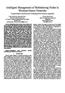
Theorem 1. Suppose that 𝐾𝑛2 /𝑃𝑛 = 𝑜(1), 𝑝𝑠 = 𝜔(1/ ln 𝑛), and 𝑛 nodes are Poissonly distributed on a unit square S with the maximum transmission radius 𝜋𝑟𝑛2 ⋅ 𝐾𝑛2 /𝑃𝑛 = (ln 𝑛 + 𝑐)/𝑛 for some constant 𝑐. Then the expected number of isolated nodes in 𝐺𝑃𝑜𝑖𝑠𝑠𝑜𝑛 (𝑛, 𝜃𝑛 , S) converges asymptotically to 𝑒−𝑐 as 𝑛 → ∞. Proof. Let 𝑊 denote the number of isolated nodes in graph V𝑥 )| 𝐺Poisson (𝑛, 𝜃𝑛 , S). By (7), we know P(𝐼𝑥 ) = ∫S 𝑒−𝑛𝑝𝑠 |𝐷𝑟𝑛 (̂ 𝑑̂ V𝑥 holds. To compute P(𝐼𝑥 ) based on S, we divide S in a way similar to that by Li et al. [35] and Wan and Yi [15]. Specially, S is divided into S0 , S1 , S2 , and S3 , respectively, as illustrated in Figure 1 (note that 𝑟𝑛 = 𝑜(1)). S0 consists of all points each with a distance greater than 𝑟𝑛 to its nearest edge to S, whereas S3 is a square of size 𝑟𝑛 ×𝑟𝑛 at the four corners of S. We further divide S\{S0 ∪S3 } into S1 and S2 as follows. In S\{S0 ∪S3 }, S1 contains points whose distance to the nearest edge of S is no greater than 𝑟𝑛 /2, while the remaining area is S2 . Then the expected number of isolated nodes is given by V𝑥 )| lim 𝐸 (𝑊) = lim 𝑛P (𝐼𝑥 ) = lim 𝑛 ∫ 𝑒−𝑛𝑝𝑠 |𝐷𝑟𝑛 (̂ 𝑑̂ V𝑥

𝑛→∞

𝑛→∞

𝑛→∞

S

V𝑥 )| = lim 𝑛 ∫ 𝑒−𝑛𝑝𝑠 |𝐷𝑟𝑛 (̂ 𝑑̂ V𝑥 𝑛→∞

S0

4

Discrete Dynamics in Nature and Society Since S1 consists of four retangles, each of which has length 1 − 2𝑟𝑛 and width 𝑟𝑛 /2, it follows that

1 rn 2

𝒮3

𝒮1

𝒮1

rn

𝒮3

𝒮2

V𝑥 )| lim 𝑛 ∫ 𝑒−𝑛𝑝𝑠 |𝐷𝑟𝑛 (̂ 𝑑̂ V𝑥

𝑛→∞

𝒮2

𝒮2

𝒮1

= 4𝑛 (1 − 2𝑟𝑛 ) lim ∫

𝒮0

1

𝑟𝑛 /2

𝑛→∞ 0

rn 2

rn 2 rn 2

𝑒

𝑑𝑔.

−1

−1

rn

𝒮3

𝒮1

(13) −𝑛𝑝𝑠 𝐻(𝑔)

For simplicity, we write 𝐻(𝑔) as 𝐻. Then

𝒮2 𝒮3

S1

−1

−1

−1

⋅ {𝑑 [(𝐻󸀠 ) 𝑒−𝑛𝑝𝑠 𝐻] − 𝑒−𝑛𝑝𝑠 𝐻𝑑 (𝐻󸀠 ) } = (𝑛𝑝𝑠 ) −1

(14)

−2

⋅ {𝑑 [− (𝐻󸀠 ) 𝑒−𝑛𝑝𝑠 𝐻] − (𝐻󸀠 ) 𝐻󸀠󸀠 𝑒−𝑛𝑝𝑠 𝐻𝑑𝑔} .

rn

rn

−1

𝑒−𝑛𝑝𝑠 𝐻(𝑔) 𝑑𝑔 = − (𝑛𝑝𝑠 ) (𝐻󸀠 ) 𝑑𝑒−𝑛𝑝𝑠 𝐻 = − (𝑛𝑝𝑠 )

Figure 1: The unit square S and its divisions S0 , S1 , S2 , and S3 .

In view of (14), we further have −2

−3

− (𝐻󸀠 ) 𝐻󸀠󸀠 𝑒−𝑛𝑝𝑠 𝐻𝑑𝑔 = − (𝐻󸀠 ) 𝐻󸀠󸀠 𝑒−𝑛𝑝𝑠 𝐻𝑑𝐻 V𝑥 )| + lim 𝑛 ∫ 𝑒−𝑛𝑝𝑠 |𝐷𝑟𝑛 (̂ 𝑑̂ V𝑥 𝑛→∞

+ lim 𝑛 ∫ 𝑒 𝑛→∞

S3

−

𝑑̂ V𝑥 . (8)

The four summands in (8) represent, respectively, the expected number of isolated nodes in the central area S0 , in the boundary area along the four sides of S, and in the four corners of S. In the following analysis, we will show that the first term approaches 𝑒−𝑐 as 𝑛 → ∞, and the remaining terms approach 0 an 𝑛 → ∞. Consider the first summand in (8). It is clear that, for any V𝑥 )| = 𝜋𝑟𝑛2 , and note that position V̂𝑥 ∈ S0 , we have |𝐷𝑟𝑛 (̂ 𝜋𝑟𝑛2 ⋅ (𝐾𝑛2 /𝑃𝑛 ) = (ln 𝑛 + 𝑐)/𝑛, |S0 | = (1 − 2𝑟𝑛 )2 to get −𝑛𝑝𝑠 |𝐷𝑟𝑛 (̂ V𝑥 )|

lim 𝑛 ∫ 𝑒

𝑛→∞

S0

−𝑛𝑝𝑠 𝜋𝑟𝑛2

= lim 𝑛𝑒 𝑛→∞

−𝑛𝑝𝑠 𝜋𝑟𝑛2

𝑑̂ V𝑥 = lim 𝑛 ∫ 𝑒 𝑛→∞

S0

−𝑐

𝑑̂ V𝑥 2

(9)

𝑛→∞

For the second term in (8), we introduce some notation as follows. For any position V̂𝑥 ∈ S1 , we let the distance from V̂𝑥 to the nearest edge of square S be 𝑔, where 0 ≤ 𝑔 ≤ 𝑟𝑛 /2. For V̂𝑥 ∈ S1 , clearly |𝐷𝑟𝑛 (̂ V𝑥 )| is determined by 𝑔, and we denote it by 𝐻(𝑔). It is easy to obtain 󵄨 󵄨 V𝑥 )󵄨󵄨󵄨󵄨 𝐻 (𝑔) = 󵄨󵄨󵄨󵄨𝐷𝑟𝑛 (̂ (10) 𝑔 = 𝜋𝑟𝑛2 − 𝑟𝑛2 arccos + 𝑔√𝑟𝑛2 − 𝑔2 , 𝑟𝑛 󸀠

𝐻 (𝑔) = 2√𝑟𝑛2 − 𝑔2 , 𝐻󸀠󸀠 (𝑔) = −

2𝑔 √𝑟𝑛2 − 𝑔2

(11) .

𝐻󸀠󸀠 3 (𝐻󸀠 )

(15) ).

=

𝑔 4 (𝑟𝑛2

−

2 𝑔2 )

≤

𝑟𝑛 /2

4×

2 ((3/4) 𝑟𝑛2 )

𝑟𝑛 /2

−∫

2 . 9𝑟𝑛3

(16)

0

−2

(𝐻󸀠 ) 𝐻󸀠󸀠 𝑒−𝑛𝑝𝑠 𝐻𝑑𝑔 (17)

𝑟𝑛 /2 2 ≤ 3 ∫ 𝑑 (−𝑒−𝑛𝑝𝑠 𝐻) . 9𝑟𝑛 𝑝𝑠 𝑛 0

Applying (17) into (14), 𝑟𝑛 /2

∫

0

𝑒−𝑛𝑝𝑠 𝐻(𝑔) 𝑑𝑔 =

−∫

𝑟𝑛 /2

0

𝑟𝑛 /2 −1 1 (∫ 𝑑 [− (𝐻󸀠 ) 𝑒−𝑛𝑝𝑠 𝐻] 𝑛𝑝𝑠 0

−2

(𝐻󸀠 ) 𝐻󸀠󸀠 𝑒−𝑛𝑝𝑠 𝐻𝑑𝑔)

≤

𝑟𝑛 /2 −1 1 (∫ 𝑑 [− (𝐻󸀠 ) 𝑒−𝑛𝑝𝑠 𝐻] 𝑛𝑝𝑠 0

+

𝑟𝑛 /2 2 𝑒−𝑛𝑝𝑠 𝐻(0) −𝑛𝑝𝑠 𝐻 𝑑 [−𝑒 ]) ≤ ∫ 9𝑟𝑛3 𝑝𝑠 𝑛 0 𝑛𝑝𝑠 𝐻󸀠 (0)

+

2𝑒−𝑛𝑝𝑠 𝐻(0) . 9𝑟𝑛3 𝑝𝑠2 𝑛2

(18)

From (10) and (11), we obtain 𝐻(0) = 𝜋𝑟𝑛2 /2 and 𝐻󸀠 (0) = 2𝑟𝑛 . Consider 𝑟𝑛 /2

∫

0

𝑒−𝑛𝑝𝑠 𝐻(𝑔) 𝑑𝑔 ≤

2𝑒−𝑛𝑝𝑠 𝐻(0) 𝑒−𝑛𝑝𝑠 𝐻(0) + 𝑛𝑝𝑠 𝐻󸀠 (0) 9𝑟𝑛3 𝑝𝑠2 𝑛2 2

(12)

=

By (15) and (16), it follows that

−𝑐

V𝑥 = lim 𝑒 (1 − 2𝑟𝑛 ) = 𝑒 . ∫ 𝑑̂ S0

−𝑛𝑝𝑠 𝐻

For 0 ≤ 𝑔 ≤ 𝑟𝑛 /2, it holds from (11) and (12) that

S2

−𝑛𝑝𝑠 |𝐷𝑟𝑛 (̂ V𝑥 )|

󸀠󸀠

= − (𝑛𝑝𝑠 ) (𝐻 ) 𝐻 𝑑 (−𝑒

S1

V𝑥 )| + lim 𝑛 ∫ 𝑒−𝑛𝑝𝑠 |𝐷𝑟𝑛 (̂ 𝑑̂ V𝑥 𝑛→∞

󸀠 −3

−1

2

𝑒−𝑛𝑝𝑠 (𝜋𝑟𝑛 /2) 2𝑒−𝑛𝑝𝑠 (𝜋𝑟𝑛 /2) = + . 2𝑟𝑛 𝑛𝑝𝑠 9𝑟𝑛3 𝑝𝑠2 𝑛2

(19)

Discrete Dynamics in Nature and Society

5

Using 𝜋𝑟𝑛2 ⋅ (𝐾𝑛2 /𝑃𝑛 ) = (ln 𝑛 + 𝑐)/𝑛 and (6) in (19), we derive ∫

𝑟𝑛 /2

0

2

𝑒−𝑛𝑝𝑠 𝐻(𝑔) 𝑑𝑔 ≤

𝑒−𝑛𝑝𝑠 (𝜋𝑟𝑛 /2) (1 + 𝑜 (1)) . 2𝑟𝑛 𝑛𝑝𝑠

(20)

lim 𝐸 (𝑊) = 𝑒−𝑐 .

−𝑛𝑝𝑠 |𝐷𝑟𝑛 (̂ V𝑥 )|

lim 𝑛 ∫ 𝑒 S1

The parameter 𝑐 in Theorem 1 is a constant, or it can depend on 𝑛, in which case 𝑐 = 𝑜(ln 𝑛). The following corollary can be established.

𝑑̂ V𝑥 𝑟𝑛 /2

= 4𝑛 (1 − 2𝑟𝑛 ) lim ∫

𝑛→∞ 0

𝑒−𝑛𝑝𝑠 𝐻(𝑔) 𝑑𝑔

(21)

2

𝑒−𝑛𝑝𝑠 (𝜋𝑟𝑛 /2) ≤ 4𝑛 lim (1 + 𝑜 (1)) . 𝑛→∞ 2𝑟 𝑛𝑝 𝑛 𝑠 From 𝐾𝑛2 /𝑃𝑛 = 𝑜(1), 𝑝𝑠 = 𝜔(1/ ln 𝑛), and with Δ denoting 𝜋𝑟𝑛2 𝑝𝑠 𝑛 (note that Δ = Θ(ln 𝑛)), 𝑟𝑛 = 𝜋−1/2 𝑝𝑠−1/2 𝑛−1/2 Δ1/2 .

(22)

V𝑥 )| lim 𝑛 ∫ 𝑒−𝑛𝑝𝑠 |𝐷𝑟𝑛 (̂ 𝑑̂ V𝑥 = 0.

(23)

We obtain 𝑛→∞

S1

V𝑥 )| 𝑑̂ V𝑥 . For V̂𝑥 ∈ Now we consider lim𝑛→∞ 𝑛 ∫S 𝑒−𝑛𝑝𝑠 |𝐷𝑟𝑛 (̂ 2 S2 , when the distance from V̂𝑥 to the nearest edge of square S V𝑥 )| is 𝑔, where 𝑟𝑛 /2 ≤ 𝑔 ≤ 𝑟𝑛 , the function expression of |𝐷𝑟𝑛 (̂ still is 𝐻(𝑔). 𝐻(𝑔) is increasing with 𝑔 for 𝑟𝑛 /2 ≤ 𝑔 ≤ 𝑟𝑛 by

𝐻󸀠 (𝑔) = 2√𝑟𝑛2 − 𝑔2 ≥ 0. Thus, when the distance from V̂𝑥 to V𝑥 )| reaches the nearest edge of S equals 𝑟𝑛 /2, the area |𝐷𝑟𝑛 (̂ its minimum value: 𝑟 2 √3 󵄨 󵄨󵄨 󵄨󵄨𝐷𝑟𝑛 (̂ V𝑥 )󵄨󵄨󵄨󵄨min = 𝐻 ( 𝑛 ) = ( + ) 𝜋𝑟𝑛2 . 󵄨 2 3 4𝜋

(24)

V𝑥 )|min = 𝐶0 𝜋𝑟𝑛2 . With 𝐶0 denoting 2/3 + √3/4𝜋, then |𝐷𝑟𝑛 (̂ And with |S2 | = 2𝑟𝑛 (1 − 2𝑟𝑛 ), we derive 2

V𝑥 )| lim 𝑛 ∫ 𝑒−𝑛𝑝𝑠 |𝐷𝑟𝑛 (̂ 𝑑̂ V𝑥 ≤ lim 𝑛 ∫ 𝑒−𝑛𝑝𝑠 𝐶0 𝜋𝑟𝑛 𝑑̂ V𝑥

𝑛→∞

𝑛→∞

S2

−𝑛𝑝𝑠 𝐶0 𝜋𝑟𝑛2

= lim 𝑛𝑒 𝑛→∞

S2

−𝑛𝑝𝑠 𝐶0 𝜋𝑟𝑛2

V𝑥 ≤ 2 lim 𝑟𝑛 𝑛𝑒 ∫ 𝑑̂ 𝑛→∞

S2

(25) .

−𝑛𝑝𝑠 |𝐷𝑟𝑛 (̂ V𝑥 )|

lim 𝑛 ∫ 𝑒 S2

𝑑̂ V𝑥 = 0.

V𝑥 )| lim 𝑛 ∫ 𝑒−𝑛𝑝𝑠 |𝐷𝑟𝑛 (̂ 𝑑̂ V𝑥 ≤ 𝑛 lim ∫ 𝑒

𝑛→∞

𝑛→∞ S 3

S3

2

= lim 𝑛𝑒−(1/4)𝑛𝑝𝑠 𝜋𝑟𝑛 ∫ 𝑑̂ V𝑥 𝑛→∞

S3

2

= lim 4𝑛𝑟𝑛2 𝑛−1/4 𝑒−(1/4)𝑛𝑝𝑠 𝜋𝑟𝑛 = 0, 𝑛→∞

Now we examine the impact of boundary effect on the number of isolated nodes in 𝐺Poisson (𝑛, 𝜃𝑛 , S) since the network area in our analysis is a square. The square accounts for the real-world boundary effect whereby some transmission region of a sensor close to the network boundary may fall outside the network field. In contrast, the torus eliminates the boundary effect. The analysis of impact of the boundary effect is done by comparing the number of isolated nodes in 𝐺Poisson (𝑛, 𝜃𝑛 , S) and the number in a network with nodes Poissonly distributed on a unit torus S𝑇 with a pair of nodes V𝑥 , V𝑦 separated by a toroidal distance ‖̂ V𝑥 − V̂𝑦 ‖𝑇 . Denote such 𝑇 network on a unit torus by 𝐺Poisson (𝑛, 𝜃𝑛 , S𝑇 ). The following Theorem can be established. Theorem 3. Suppose that 𝐾𝑛2 /𝑃𝑛 = 𝑜(1), 𝑝𝑠 = 𝜔(1/ ln 𝑛), and 𝑛 nodes are Poissonly distributed on a unit torus S𝑇 with the maximum transmission radius 𝜋𝑟𝑛2 ⋅ (𝐾𝑛2 /𝑃𝑛 ) = (ln 𝑛 + 𝑐)/𝑛 for some constant 𝑐. Then the expected number of isolated nodes in 𝑇 (𝑛, 𝜃𝑛 , S𝑇 ) converges to 𝑒−𝑐 as 𝑛 → ∞. 𝐺𝑃𝑜𝑖𝑠𝑠𝑜𝑛 Proof. Let 𝑊𝑇 denote the number of isolated nodes in graph 𝑇 𝐺Poisson (𝑛, 𝜃𝑛 , S𝑇 ), and let 𝐷𝑟𝑇𝑛 (̂ V𝑥 ) denote the intersection 𝑇 of S and the disk centered at position V̂𝑥 ∈ S𝑇 with radius 𝑟𝑛 . The probability that node V𝑥 is isolated is P(𝐼𝑥𝑇) = 𝑇 V𝑥 )| 𝑑̂ V𝑥 . Since S𝑇 is a unit torus, it holds that ∫S𝑇 𝑒−𝑛𝑝𝑠 |𝐷𝑟𝑛 (̂ 𝑇 2 |𝐷𝑟𝑛 (̂ V𝑥 )| = 𝜋𝑟𝑛 for any V̂𝑥 ∈ S𝑇 . Then 𝑇

2

S𝑇

S𝑇

−𝜋𝑟𝑛2 𝑝𝑠 𝑛

=𝑒

(26)

V𝑥 )| ≤ For the last term in (8), we have (1/4)𝜋𝑟𝑛2 ≤ |𝐷𝑟𝑛 (̂ 2 2 𝜋𝑟𝑛 for any V̂𝑥 ∈ S3 and |S3 | = 4𝑟𝑛 to get −(1/4)𝑛𝑝𝑠 𝜋𝑟𝑛2

Corollary 2. In graph 𝐺𝑃𝑜𝑖𝑠𝑠𝑜𝑛 (𝑛, 𝜃𝑛 , S) under conditions 𝐾𝑛2 /𝑃𝑛 = 𝑜(1), 𝑝𝑠 = 𝜔(1/ ln 𝑛), and 𝜋𝑟𝑛2 ⋅(𝐾𝑛2 /𝑃𝑛 ) = (ln 𝑛 + 𝑐)/𝑛 with 𝑐 = 𝑜(ln 𝑛) or a constant 𝑐, then for any constant 𝜖 > 0 such that 𝐸(𝑊) = 𝑜(𝑛𝜖 ) holds.

V𝑥 )| P (𝐼𝑥𝑇 ) = ∫ 𝑒−𝑛𝑝𝑠 |𝐷𝑟𝑛 (̂ 𝑑̂ V𝑥 = 𝑒−𝜋𝑟𝑛 𝑝𝑠 𝑛 ∫ 𝑑̂ V𝑥

From 𝑝𝑠 = 𝜔(1/ ln 𝑛), Δ = Θ(ln 𝑛), and (22), it follows 𝑛→∞

(28)

𝑛→∞

Using (20) in (13), we get 𝑛→∞

where (22), Δ = Θ(ln 𝑛), and 𝑝𝑠 = 𝜔(1/ ln 𝑛) are used in reaching (27). As a result of (8),(9), (23), (26), and (27), we prove

󵄨 󵄨 ⋅ 󵄨󵄨󵄨󵄨S𝑇 󵄨󵄨󵄨󵄨 = 𝑒

−𝜋𝑟𝑛2 𝑝𝑠 𝑛

(29)

.

Using the condition 𝜋𝑟𝑛2 ⋅ (𝐾𝑛2 /𝑃𝑛 ) = (ln 𝑛 + 𝑐)/𝑛, we obtain 2

lim 𝐸 (𝑊𝑇 ) = lim 𝑛P (𝐼𝑥𝑇 ) = lim 𝑛𝑒−𝜋𝑟𝑛 𝑝𝑠 𝑛 = 𝑒−𝑐 .

𝑛→∞

𝑛→∞

𝑛→∞

(30)

𝑑̂ V𝑥 (27)

On the basis of Theorems 1 and 3, using the coupling technique, the following theorem can be obtained. Theorem 4. Suppose that 𝐾𝑛2 /𝑃𝑛 = 𝑜(1), 𝑝𝑠 = 𝜔(1/ ln 𝑛), and 𝑛 nodes are Poissonly distributed on a unit square S

6

Discrete Dynamics in Nature and Society

with the maximum transmission radius 𝜋𝑟𝑛2 ⋅ (𝐾𝑛2 /𝑃𝑛 ) = (ln 𝑛 + 𝑐)/𝑛 for some constant 𝑐. Then the number of isolated nodes in 𝐺𝑃𝑜𝑖𝑠𝑠𝑜𝑛 (𝑛, 𝜃𝑛 , S) due to the boundary effect converges asymptotically to 0 as 𝑛 → ∞. Proof. Comparing Theorems 1 and 3, it is noted that the expected numbers of isolated nodes on a unit torus S𝑇 and on a unit square S, respectively, asymptotically converge to the same constant 𝑒−𝑐 as 𝑛 → ∞. Now we use the coupling technique [36] to construct the connection between 𝑇 𝑊 and 𝑊𝑇 . Consider a graph 𝐺Poisson (𝑛, 𝜃𝑛 , S𝑇 ), and the number of isolated nodes in that graph is 𝑊𝑇 . Remove each connection of the above graph with probability 1 − |𝐷𝑟𝑛 (̂ V𝑥 )|/|𝐷𝑟𝑇𝑛 (̂ V𝑥 )|, independently of the event that another V𝑥 )| ≤ |𝐷𝑟𝑇𝑛 (̂ V𝑥 )|, then connection is removed. Due to |𝐷𝑟𝑛 (̂ 𝑇 V𝑥 )|/|𝐷𝑟𝑛 (̂ V𝑥 )| ≤ 1. We further note that 0 ≤ 1 − |𝐷𝑟𝑛 (̂ only connections between nodes near the boundary will be affected. Denote the number of newly appearing isolated nodes by 𝑊𝐸 ; namely, 𝑊𝐸 is the number of isolated nodes due to the boundary effect; it is straightforward to show that 𝑊𝐸 is a nonnegative random integer. Further, such a connection removal process results in a random network with nodes Poissonly distributed with density 𝑛. That is, a random network on a unit square with boundary effect is included. The following equation result holds: 𝑊 = 𝑊𝐸 + 𝑊𝑇 .

Lemma 5 (see [37, 38]). Suppose that 𝑌 = ∑𝑎∈Γ 𝐼𝑎 , where the indicator variables (𝐼𝑎 )𝑎∈Γ are positively related random indicator variables. Then one has 𝑑𝑇𝑉 (𝑌, Poi (𝐸𝑌)) ≤

1 − 𝑒−𝐸𝑌 2 (Var 𝑌 − 𝐸𝑌 + 2∑ (𝐸𝐼𝑎 ) ) . 𝐸𝑌 𝑎∈Γ

For 𝑥 = 1, . . . , 𝑛, let 𝐼𝑥𝑇 = 1 if node V𝑥 is isolated in 𝑇 (𝑛, 𝜃𝑛 , S𝑇 ) and 𝑊𝑇 = ∑𝑛𝑥=1 𝐼𝑥𝑇 . Therefore, 𝑊𝑇 is the 𝐺Poisson 𝑇 (𝑛, 𝜃𝑛 , S𝑇 ) as defined number of isolated nodes in 𝐺Poisson in Theorem 3. We will demonstrate the asymptotic Poisson distribution of 𝑊𝑇 by employing the Stein-Chen method [37]. The result is given in Theorem 6. Theorem 6. Suppose 𝐾𝑛 ≥ ln 𝑛/ ln ln 𝑛, 𝐾𝑛2 /𝑃𝑛 = 𝑜(1), 𝑝𝑠 = 𝜔(1/ ln 𝑛), and 𝑛 nodes are Poissonly distributed on a unit torus S𝑇 with the maximum transmission radius 𝜋𝑟𝑛2 ⋅ (𝐾𝑛2 /𝑃𝑛 ) = (ln 𝑛 + 𝑐)/𝑛 for some constant 𝑐. Then the distribution of the 𝑇 number of isolated nodes in 𝐺𝑃𝑜𝑖𝑠𝑠𝑜𝑛 (𝑛, 𝜃𝑛 , S𝑇 ) converges to a −𝑐 Poisson distribution with mean 𝑒 as 𝑛 → ∞. Proof. The triangular inequality for the total variation distance implies 𝑑𝑇𝑉 (𝑊𝑇 , Poi (𝑒−𝑐 ))

(31)

≤ 𝑑𝑇𝑉 (𝑊𝑇 , Poi (𝐸𝑊𝑇 ))

𝑇

lim 𝐸 (𝑊 ) = lim 𝐸 (𝑊 − 𝑊 ) = 0.

𝑛→∞

𝑛→∞

(32)

Due to the nonnegativity of 𝑊𝐸 , lim P (𝑊𝐸 = 0) = 1.

𝑛→∞

By a coupling argument [39] and Theorem 3, we have 󵄨 󵄨 𝑑𝑇𝑉 (Poi (𝐸𝑊𝑇 ) , Poi (𝑒−𝑐 )) ≤ 󵄨󵄨󵄨󵄨𝐸𝑊𝑇 − 𝑒−𝑐 󵄨󵄨󵄨󵄨 = 𝑜 (1) . (37) Combining this with (36), we now only need to prove lim 𝑑 (𝑊𝑇 , Poi (𝐸𝑊𝑇 )) 𝑛→∞ 𝑇𝑉

(33)

= 0.

(38)

First, we claim that (𝐼𝑥𝑇 )𝑛𝑥=1 are positively related. To see this, define

3.2. Distribution of the Number of Isolated Nodes in 𝐺𝑃𝑜𝑖𝑠𝑠𝑜𝑛 (𝑛, 𝜃𝑛 , S). In this subsection, we analyze the distribution of the number of isolated nodes in 𝐺Poisson (𝑛, 𝜃𝑛 , S). For this purpose, we give some definitions. Let Poi(𝜆) be a Poisson random variable with parameter 𝜆. Let Γ be a finite set of indices and let (𝐼𝑎 )𝑎∈Γ be a family of random indicator variables. We say (𝐼𝑎 )𝑎∈Γ are positively related (see [37]), if, for each 𝑎 ∈ Γ, there exist random indicator variables (𝐽𝑏𝑎 )𝑏∈Γ\{𝑎} with the distributions L ((𝐽𝑏𝑎 )𝑏∈Γ\{𝑎} ) = L ((𝐼𝑏 )𝑏∈Γ\{𝑎} | 𝐼𝑎 = 1) ,

(36)

+ 𝑑𝑇𝑉 (Poi (𝐸𝑊𝑇 ) , Poi (𝑒−𝑐 )) .

By Theorems 1 and 3 and the above equation, it can be shown that 𝐸

(35)

(34)

𝑇 =1 𝐼𝑦𝑥 𝑇 (𝑛, 𝜃𝑛󸀠 , S𝑇1 ) , if node V𝑦 is isolated in 𝐺Poisson

𝑇 (𝑛, 𝜃𝑛󸀠 , S𝑇1 ) is a graph with 𝑃𝑛 \|𝑆𝑥 | or S𝑇1 = S𝑇 \ where 𝐺Poisson 𝑇 𝑇 V𝑥 ) compared to 𝐺Poisson (𝑛, 𝜃𝑛 , S𝑇 ), where 𝑆𝑥 represents 𝐷𝑟𝑛 (̂ 𝑇 (𝑛, 𝜃𝑛 , S𝑇 ). the key ring which is adjacent to V𝑥 in 𝐺Poisson 𝑇 Conditional on the isolation of node V𝑥 in 𝐺Poisson (𝑛, 𝜃𝑛 , S𝑇 ), V𝑥 ) in any node V𝑦 is not adjacent to 𝑆𝑥 or V̂𝑦 ∈ S𝑇 \ 𝐷𝑟𝑇𝑛 (̂ 𝑇 (𝑛, 𝜃𝑛 , S𝑇 ). Hence, we have 𝐺Poisson 𝑛

𝑇 ) L ((𝐼𝑦𝑥

𝑦=1,𝑦=𝑥 ̸

such that 𝐽𝑏𝑎 ≥ 𝐼𝑏 for every 𝑏 ≠ 𝑎. A useful result obtained by Stein-Chen method is the following.

(39)

𝑛

) = L ((𝐼𝑦𝑇 )

𝑦=1,𝑦=𝑥 ̸

| 𝐼𝑥𝑇 = 1) .

(40)

𝑇 For every 𝑦 ≠ 𝑥, if 𝐼𝑦𝑇 = 1 then 𝐼𝑦𝑥 = 1. Consequently, we get 𝑇 𝑇 𝐼𝑦𝑥 ≥ 𝐼𝑦 .

Discrete Dynamics in Nature and Society

7

By Lemma 5, the binary nature, and exchangeability of the random variables involved, we find that 𝑑𝑇𝑉 (𝑊𝑇 , Poi (𝐸𝑊𝑇 )) 𝑇

≤

𝑛 2 1 − 𝑒−𝐸𝑊 (Var 𝑊𝑇 − 𝐸𝑊𝑇 + 2 ∑ (𝐸𝐼𝑥𝑇 ) ) 𝑇 𝐸𝑊 𝑥=1

≤

𝑛 2 1 (Var 𝑊𝑇 − 𝐸𝑊𝑇 + 2 ∑ (𝐸𝐼𝑥𝑇 ) ) 𝑇 𝐸𝑊 𝑥=1

≤

2 1 (𝑛 (𝑛 − 1) 𝐸 (𝐼𝑥𝑇 𝐼𝑦𝑇 ) − 𝑛 (𝑛 − 2) (𝐸𝐼𝑥𝑇 ) ) . 𝑇 𝐸𝑊

isolated nodes for 𝐺(𝑛, 𝜃𝑛 , S) follows once we establish the result with Poissonization, that is to say, once we obtain the distribution of isolated nodes for 𝐺Poisson (𝑛, 𝜃𝑛 , S). See the following lemma for rigorous argument.

(41)

Lemma 8. Suppose that 𝐾𝑛2 /𝑃𝑛 = 𝑜(1), 𝑝𝑠 = 𝜔(1/ ln 𝑛), and 𝑛 nodes have the same maximum transmission radius 𝜋𝑟𝑛2 ⋅ (𝐾𝑛2 /𝑃𝑛 ) = (ln 𝑛 + 𝑐)/𝑛 for some constant 𝑐. Then with 𝑚 denoting ⌈𝑛 − 𝑛1/2+𝑐0 ⌉, where 𝑐0 is an arbitrary constant with 0 < 𝑐0 < 1/2, then node V𝑖 is isolated in 𝐺(𝑛, 𝜃𝑛 , S) if and only if V𝑖 is an isolated node in 𝐺𝑃𝑜𝑖𝑠𝑠𝑜𝑛 (𝑚, 𝜃𝑛 , S).

The cross term 𝐸(𝐼𝑥𝑇𝐼𝑦𝑇 ) in (41) is given by [33], and we have

Proof. We will use the standard de-Poissonization technique [11, 14, 18] to prove Lemma 8. Let 𝑀 denote the number of nodes in graph 𝐺Poisson (𝑚, 𝜃𝑛 , S); clearly 𝑀 follows a Poisson distribution with mean 𝑚, for any positive 𝑡, and from Chebyshev’s inequality, we have

𝐸 (𝐼𝑥𝑇 𝐼𝑦𝑇 ) 2

≤ (1 − 4𝜋𝑟𝑛2 ) 𝑒−2𝜋𝑟𝑛 𝑝𝑠 𝑛 2

2

4

2

𝜋𝑟𝑛2 𝑛(𝐾𝑛 /𝑃𝑛 )

2

+ 4𝜋𝑟𝑛2 𝑒−2𝜋𝑟𝑛 𝑝𝑠 𝑛 𝑒2𝜋𝑟𝑛 𝑛(𝐾𝑛 /𝑃𝑛 )+(𝐾𝑛 /(𝑃𝑛 −𝐾𝑛 ))𝑒 2

4

2

2

𝜋𝑟𝑛2 𝑛(𝐾𝑛 /𝑃𝑛 )

With 𝐹(𝑛) denoting 𝑒2𝜋𝑟𝑛 𝑛(𝐾𝑛 /𝑃𝑛 )+(𝐾𝑛 /(𝑃𝑛 −𝐾𝑛 ))𝑒 ing (29), (41), and (42) readily gives

.

, combin-

𝑑𝑇𝑉 (𝑊𝑇 , Poi (𝐸𝑊𝑇 )) 2

𝑛 [(𝑛 − 1) 𝑒−2𝜋𝑟𝑛 𝑝𝑠 𝑛 (1 + 4𝜋𝑟𝑛2 𝐹 (𝑛)) − (𝑛 − 2) 𝑒−2𝜋𝑟𝑛 𝑝𝑠 𝑛 ] 2

≤

𝑛𝑒−2𝜋𝑟𝑛 𝑝𝑠 𝑛 (1 + 4𝑛𝜋𝑟𝑛2 𝐹 (𝑛)) 𝑛𝑒

≤𝑒

(45)

(43)

−𝜋𝑟𝑛2 𝑝𝑠 𝑛

−𝜋𝑟𝑛2 𝑝𝑠 𝑛

𝑛 − 𝑛1/2+𝑐0 𝑛1+2𝑐0

= 𝑜 (1) .

2

𝑛𝑒−𝜋𝑟𝑛 𝑝𝑠 𝑛

(44)

Without loss of generality, we take 𝑛 − 𝑛1/2+𝑐0 as an integer. With 𝑡 = (𝑛 − 𝑚)/√𝑚, substituting 𝑚 = 𝑛 − 𝑛1/2+𝑐0 into (46), we get P (𝑀 ≤ 𝑛 − 2𝑛1/2+𝑐0 or 𝑀 ≥ 𝑛) ≤

2

≤

P (|𝑀 − 𝑚| ≥ 𝑡√𝑚) ≤ 𝑡−2 .

(42)

(1 + 4𝑛𝜋𝑟𝑛2 𝐹 (𝑛)) = 𝑜 (1) ,

where 𝐾𝑛 ≥ ln 𝑛/ ln ln 𝑛, 𝐾𝑛2 /𝑃𝑛 = 𝑜(1), 𝑝𝑠 = 𝜔(1/ ln 𝑛) 𝜋𝑟𝑛2 ⋅ (𝐾𝑛2 /𝑃𝑛 ) = (ln 𝑛 + 𝑐)/𝑛, and (22) are used in reaching (43), along with (36), (37), and (43), which concludes the proof. We now consider the asymptotic distribution of the number of isolated nodes in 𝐺Poisson (𝑛, 𝜃𝑛 , S). From Theorem 4, lim𝑛→∞ P(𝑊𝐸 = 0) = 1 holds, and using Slutsky’s Theorem [40], the following result on the asymptotic distribution of 𝑊 can be readily obtained. Theorem 7. Suppose 𝐾𝑛 ≥ ln 𝑛/ ln ln 𝑛, 𝐾𝑛2 /𝑃𝑛 = 𝑜(1), 𝑝𝑠 = 𝜔(1/ ln 𝑛), and 𝑛 nodes are Poissonly distributed on a unit square S with the maximum transmission radius 𝜋𝑟𝑛2 ⋅ (𝐾𝑛2 /𝑃𝑛 ) = (ln 𝑛 + 𝑐)/𝑛 for some constant 𝑐. Then the distribution of the number of isolated nodes in 𝐺𝑃𝑜𝑖𝑠𝑠𝑜𝑛 (𝑛, 𝜃𝑛 , S) converges to a Poisson distribution with mean 𝑒−𝑐 as 𝑛 → ∞. 3.3. Distribution of the Number of Isolated Nodes in 𝐺(𝑛, 𝜃𝑛 , S). We derive the distribution of isolated nodes in 𝐺(𝑛, 𝜃𝑛 , S) by using standard Poissonization technique [11, 14]. The idea is that the result about the distribution of

Hence, 𝑛 − 2𝑛1/2+𝑐0 < 𝑀 < 𝑛 holds almost surely. When 𝑀 < 𝑛, we construct a coupling C between graph 𝐺(𝑛, 𝜃𝑛 , S) and graph 𝐺Poisson (𝑚, 𝜃𝑛 , S); let graph 𝐺(𝑛, 𝜃𝑛 , S) be the result of adding 𝑛 − 𝑀 nodes uniformly distributed on S to graph 𝐺Poisson (𝑚, 𝜃𝑛 , S). Let 𝑉𝑃 be the node set of 𝐺Poisson (𝑚, 𝜃𝑛 , S); clearly, 𝑉𝑃 is a subset of 𝑉, where 𝑉 is the node set of 𝐺(𝑛, 𝜃𝑛 , S). In addition, it is straightforward to see that the edge set of 𝐺Poisson (𝑚, 𝜃𝑛 , S) is also a subset of that of 𝐺(𝑛, 𝜃𝑛 , S). Then under coupling C, graph 𝐺Poisson (𝑚, 𝜃𝑛 , S) is a subgraph of 𝐺(𝑛, 𝜃𝑛 , S). Let 𝐷𝑋 , 𝐷𝑃 denote the set of isolated nodes in 𝐺(𝑛, 𝜃𝑛 , S) and 𝐺Poisson (𝑚, 𝜃𝑛 , S), respectively. To prove Lemma 8, we show P (𝐷𝑋 ≠ 𝐷𝑃 ) = 𝑜 (1) .

(46)

It is straightforward to see P (𝐷𝑋 ≠ 𝐷𝑃 ) ≤ P [(𝐷𝑃 \ 𝐷𝑋 ≠ 0) ∩ (𝑛 − 2𝑛1/2+𝑐0 < 𝑀 < 𝑛)] + P [(𝐷𝑋 \ 𝐷𝑃 ≠ 0) ∩ (𝑛 − 2𝑛1/2+𝑐0 < 𝑀 < 𝑛)] + P (𝑀 ≤ 𝑛 − 2𝑛1/2+𝑐0 or 𝑀 ≥ 𝑛) .

(47)

8

Discrete Dynamics in Nature and Society

By (47), we will prove P(𝐷𝑋 ≠ 𝐷𝑃 ) = 𝑜(1) if we can derive P [(𝐷𝑃 \ 𝐷𝑋 ≠ 0) ∩ (𝑛 − 2𝑛1/2+𝑐0 < 𝑀 < 𝑛)] = 𝑜 (1) , P [(𝐷𝑋 \ 𝐷𝑃 ≠ 0) ∩ (𝑛 − 2𝑛1/2+𝑐0 < 𝑀 < 𝑛)] = 𝑜 (1) .

(48)

(49)

To prove (48) and (49), with 𝑛−2𝑛1/2+𝑐0 < 𝑀 < 𝑛, we consider the coupling C under which 𝐺Poisson (𝑚, 𝜃𝑛 , S) is a subgraph of 𝐺(𝑛, 𝜃𝑛 , S). First, we consider (48) with 𝑛 − 2𝑛1/2+𝑐0 < 𝑀 < 𝑛; event 𝐷𝑃 \ 𝐷𝑋 ≠ 0 happens if and only if there exists at least one node V𝑖 such that V𝑖 ∈ 𝐷𝑃 and V𝑖 ∉ 𝐷𝑋 ; that is to say, V𝑖 is isolated in 𝐺Poisson (𝑚, 𝜃𝑛 , S) but is not isolated in 𝐺(𝑛, 𝜃𝑛 , S). Then there exists at least one node V󸀠 in 𝑉 \ 𝑉𝑃 such that V󸀠 and V𝑖 are neighbors in 𝐺(𝑛, 𝜃𝑛 , S). Due to |𝑉 \ 𝑉𝑃 | = 𝑛 − 𝑀 < 2𝑛1/2+𝑐0 , noting that 𝑝𝑒 is the edge probability in 𝐺(𝑛, 𝜃𝑛 , S), then with 𝑊𝑃 denoting the number of isolated nodes in 𝐺Poisson (𝑚, 𝜃𝑛 , S), as an easy consequence of the union bound, P [(𝐷𝑃 \ 𝐷𝑋 ≠ 0) ∩ (𝑛 − 2𝑛

1/2+𝑐0

< 𝑀 < 𝑛)] (50)

≤ 𝑊𝑃 ⋅ 2𝑛1/2+𝑐0 ⋅ 𝑝𝑒 .

In order to apply Corollary 2 to 𝐺Poisson (𝑚, 𝜃𝑛 , S), for 𝑛 sufficiently large, the following condition holds: 𝜋𝑟𝑛2 ⋅

𝐾𝑛2 ln 𝑚 + 𝑐 = . 𝑃𝑛 𝑚

(51)

𝐾𝑛2 ln 𝑛 + 𝑐 − (ln 𝑚 + 𝑐) = 𝑚 ⋅ − (ln 𝑚 + 𝑐) 𝑃𝑛 𝑛

= (𝑛 − 𝑛1/2+𝑐0 ) ⋅

ln 𝑛 + 𝑐 − (ln (𝑛 − 𝑛1/2+𝑐0 ) + 𝑐) 𝑛

(52)

= (1 − 𝑛𝑐0 −1/2 ) (ln 𝑛 + 𝑐) − ln 𝑛 − ln (1 − 𝑛𝑐0 −1/2 ) − 𝑐 = 𝑜 (1) , where 0 < 𝑐0 < 1/2. And sufficiently large 𝑛 are used in the final step. Then with (51), for any constant 𝜖 > 0, we use Corollary 2 to get 𝜖

𝜖

𝑊𝑃 = 𝑜 (𝑚 ) = 𝑜 (𝑛 ) .

(53)

Note that 𝑝𝑒 ≤ 𝜋𝑟𝑛2 ⋅ 𝑝𝑠 , and 𝜋𝑟𝑛2 ⋅ (𝐾𝑛2 /𝑃𝑛 ) = ((ln 𝑛 + 𝑐)/𝑛). Then from (50), with 𝜖 satisfying 0 < 𝜖 < 1/2 − 𝑐0 , it follows that P [(𝐷𝑃 \ 𝐷𝑋 ≠ 0) ∩ (𝑛 − 2𝑛1/2+𝑐0 < 𝑀 < 𝑛)] ≤ 𝑜 (𝑛𝜖 ) ⋅ 2𝑛1/2+𝑐0 ⋅

ln 𝑛 + 𝑐 = 𝑜 (1) . 𝑛

P [(𝐷𝑋 \ 𝐷𝑃 ≠ 0) ∩ (𝑛 − 2𝑛1/2+𝑐0 < 𝑀 < 𝑛)] ≤ 2𝑛1/2+𝑐0 ⋅ 𝑞.

(55)

V𝑥 )| Since 𝑞 = ∫S 𝑒−𝑛𝑝𝑠 |𝐷𝑟𝑛 (̂ 𝑑̂ V𝑥 , according to the proof of Theorem 1, it is easy to show 𝑞 = Θ(ln 𝑛/𝑛). With 𝑞 = Θ(ln 𝑛/𝑛) and 0 < 𝑐0 < 1/2, then

P [(𝐷𝑋 \ 𝐷𝑃 ≠ 0) ∩ (𝑛 − 2𝑛1/2+𝑐0 < 𝑀 < 𝑛)] = 𝑜 (1) .

(56)

In conclusion, since |P(𝐷𝑋 ≠ 0) − P(𝐷𝑃 ≠ 0)| ≤ P(𝐷𝑋 ≠ 𝐷𝑃 ), the above discussions lead to establish Lemma 8. Applying Theorem 7 and Lemma 8, we get the following theorem. Theorem 9. Suppose 𝐾𝑛 ≥ ln 𝑛/ ln ln 𝑛, 𝐾𝑛2 /𝑃𝑛 = 𝑜(1), 𝑝𝑠 = 𝜔(1/ ln 𝑛), and 𝑛 nodes are uniformly distributed on a unit square S with the maximum transmission radius 𝜋𝑟𝑛2 ⋅ (𝐾𝑛2 /𝑃𝑛 ) = (ln 𝑛 + 𝑐)/𝑛 for some constant 𝑐. Then the distribution of the number of isolated nodes in 𝐺(𝑛, 𝜃𝑛 , S) converges to a Poisson distribution with mean 𝑒−𝑐 as 𝑛 → ∞. Noting that the number of isolated nodes in a network is a nonnegative integer, the following result can be obtained as a consequence of Theorems 7 and 9. Notice that, in formulating this result, we drop the assumption that 𝑐 originally is a constant and allow it instead to be 𝑛-dependent.

We demonstrate (51) in view of 𝑚 ⋅ 𝜋𝑟𝑛2 ⋅

Second, in order to prove (49) with 𝑛 − 2𝑛1/2+𝑐0 < 𝑀 < 𝑛, we consider event that 𝐷𝑋 \ 𝐷𝑃 ≠ 0 occurs if and only if there exists at least one node V𝑗 such that V𝑗 ∈ 𝐷𝑋 and V𝑗 ∉ 𝐷𝑃 . With V𝑗 ∈ 𝐷𝑋 , then V𝑗 is isolated in 𝐺(𝑛, 𝜃𝑛 , S), which along with V𝑗 ∉ 𝐷𝑃 leads to V𝑗 ∉ 𝑉𝑃 and V𝑗 ∈ 𝑉 \ 𝑉𝑃 . Let 𝑞 denote the probability that a node is isolated in 𝐺(𝑛, 𝜃𝑛 , S); it follows via a union bound that

(54)

Corollary 10. Suppose 𝐾𝑛2 /𝑃𝑛 = 𝑜(1), 𝑝𝑠 = 𝜔(1/ ln 𝑛), and 𝑛 nodes are Poissonly (uniformly) distributed on a unit square S with the maximum transmission radius 𝜋𝑟𝑛2 ⋅ (𝐾𝑛2 /𝑃𝑛 ) = (ln 𝑛 + 𝑐𝑛 )/𝑛 for some 𝑐𝑛 . A necessary condition for graph 𝐺𝑃𝑜𝑖𝑠𝑠𝑜𝑛 (𝑛, 𝜃𝑛 , S)(𝐺(𝑛, 𝜃𝑛 , S)) to be asymptotically connected is 𝑐𝑛 → ∞.

4. Conclusion and Future Work Yi et al. [10] considered that a wireless ad hoc network consists of 𝑛 nodes distributed independently and uniformly in a unit disk D or a unit square S. They used Brun’s sieve to show that, for graph 𝐺(𝑛, 𝜃𝑛 , D) or 𝐺(𝑛, 𝜃𝑛 , S), if 𝜋𝑟𝑛2 ⋅ (𝐾𝑛2 /𝑃𝑛 ) = (ln 𝑛 + 𝑐)/𝑛 and 𝐾𝑛2 /𝑃𝑛 = 𝜔(1/ ln 𝑛), the number of isolated nodes asymptotically follows a Poisson distribution with mean 𝑒−𝑐 . Pishro-Nik et al. [34] also obtained such result on asymptotic Poisson distribution with condition 𝐾𝑛2 /𝑃𝑛 = 𝜔(1/ ln 𝑛) generalized to 𝐾𝑛2 /𝑃𝑛 = Ω(1/ ln 𝑛). In this paper, we discuss the distribution of isolated nodes in WSNs employing the widely Eschenauer-Gligor key

Discrete Dynamics in Nature and Society

9

predistribution scheme under transmission constraint with nodes distributed either Poissonly or uniformly on a unit square S or a unit torus S𝑇 . Using the coupling technique, it is shown that the impact of the boundary effect on the number of isolated nodes vanishes small as 𝑛 → ∞. We obtain that the numbers of isolated nodes in graph 𝐺(𝑛, 𝜃𝑛 , S) and graph 𝐺Poisson (𝑛, 𝜃𝑛 , S) asymptotically follow a Poisson distribution with mean 𝑒−𝑐 with 𝜋𝑟𝑛2 ⋅ (𝐾𝑛2 /𝑃𝑛 ) = (ln 𝑛 + 𝑐)/𝑛 and 𝐾𝑛2 /𝑃𝑛 = 𝜔(1/ ln 𝑛). In practice WSNs, 𝐾𝑛 is expected to be several orders of magnitude smaller than 𝑃𝑛 , so it often holds that 𝐾𝑛2 /𝑃𝑛 = 𝑜(1/ ln 𝑛). We believe that the following conjecture is true. Conjecture 11. Suppose that 𝐾𝑛2 /𝑃𝑛 = 𝑜(1), 𝐾𝑛2 /𝑃𝑛 = 𝑜(1/ ln 𝑛), and 𝑛 nodes are uniformly (Poissonly) distributed on a unit square S with the maximum transmission radius 𝜋𝑟𝑛2 ⋅ (𝐾𝑛2 /𝑃𝑛 ) = (ln 𝑛 + 𝑐)/𝑛 for some constant 𝑐. Then the distribution of the number of isolated nodes in graph 𝐺(𝑛, 𝜃𝑛 , S) (graph 𝐺𝑃𝑜𝑖𝑠𝑠𝑜𝑛 (𝑛, 𝜃𝑛 , S)) converges to a Poisson distribution with mean 𝑒−𝑐 as 𝑛 → ∞. Connectivity in secure wireless sensor networks under transmission constraints is another important subject. Although the significant improved conditions and results for asymptotic connectivity are presented by Krishnan et al. [4], Krzywdzi´nski and Rybarczyk [13], Tang and Li [32], and Zhao et al. [33], we want to show that the connectivity in WSN with the EG scheme (i.e., 𝐺(𝑛, 𝜃𝑛 , S)) is exactly analogue of the counterpart in classic random graphs. Conjecture 12. Suppose that 𝐾𝑛2 /𝑃𝑛 = 𝑜(1), 𝐾𝑛2 /𝑃𝑛 𝑜(1/ ln 𝑛), and 𝜋𝑟𝑛2 ⋅ (𝐾𝑛2 /𝑃𝑛 ) = (ln 𝑛 + 𝑐𝑛 )/𝑛.

=

(i) If 𝑐𝑛 → −∞, then with high probability 𝐺(𝑛, 𝜃𝑛 , S) is disconnected. (ii) If 𝑐𝑛 → 𝑐, then the probability that 𝐺(𝑛, 𝜃𝑛 , S) is −𝑐 connected tends to 𝑒−𝑒 . (iii) If 𝑐𝑛 → ∞, then with high probability 𝐺(𝑛, 𝜃𝑛 , S) is connected. It would be interesting to carry out an illustrative simulation to strengthen the theoretical asymptotic results of the distribution of the number of isolated nodes and connectivity. The simulations may be carried out for small, medium, and large but not very large networks. Such results hold under condition 𝐾𝑛2 /𝑃𝑛 = 𝑜(1/ ln 𝑛), which remains an open research challenge.

Competing Interests The authors declare that they have no competing interests.

Acknowledgments The work was supported by National Natural Science Foundation of China (NSFC) under Grant no. 11071272 and the project sponsored by the Scientific Research Foundation for the Returned Overseas Scholars of the Education Ministry of China.

References [1] E. N. Gilbert, “Random plane networks,” Journal of the Society for the Industrial and Applied Mathematics, vol. 9, pp. 533–543, 1961. [2] L. Eschenauer and V. D. Gligor, “A key-management scheme for distributed sensor networks,” in Proceedings of the 9th ACM Conference on Computer and Communications Security (CCS ’02), pp. 41–47, ACM Press, Washington, DC, USA, November 2002. [3] H. Chan, A. Perrig, and D. Song, “Random key predistribution schemes for sensor networks,” in Proceedings of the Symposium on Security and Privacy (SP ’03), pp. 197–213, IEEE, Berkeley, Calif, USA, May 2003. [4] B. S. Krishnan, A. Ganesh, and D. Manjunath, “On connectivity thresholds in superposition of random key graphs on random geometric graphs,” in Proceedings of the IEEE International Symposium on Information Theory (ISIT ’13), pp. 2389–2393, Istanbul, Turkey, July 2013. [5] K. Rybarczyk, “Diameter, connectivity, and phase transition of the uniform random intersection graph,” Discrete Mathematics, vol. 311, no. 17, pp. 1998–2019, 2011. [6] O. Yagan and A. M. Makowski, “Zero-one laws for connectivity in random key graphs,” IEEE Transactions on Information Theory, vol. 58, no. 5, pp. 2983–2999, 2012. [7] S. R. Blackburn and S. Gerke, “Connectivity of the uniform random intersection graph,” Discrete Mathematics, vol. 309, no. 16, pp. 5130–5140, 2009. [8] M. Bloznelis, “Degree and clustering coefficient in sparse random intersection graphs,” The Annals of Applied Probability, vol. 23, no. 3, pp. 1254–1289, 2013. [9] J. Zhao, O. Ya˘gan, and V. Gligor, “k-connectivity in secure wireless sensor networks with physical link constraints-the On/Off channel model,” https://arxiv.org/abs/1206.1531. [10] C.-W. Yi, P.-J. Wan, K.-W. Lin, and C.-H. Huang, “WSN185: asymptotic distribution of the number of isolated nodes in wireless ad hoc networks with unreliable nodes and links,” in Proceedings of the IEEE GLOBECOM, pp. 1–5, San Francisco, Calif, USA, November-December 2006. [11] M. D. Penrose, Random Geometric Graphs, vol. 5 of Oxford Studies in Probability, Oxford University Press, Oxford, UK, 2003. [12] P. Gupta and P. R. Kumar, “Critical power for asymptotic connectivity in wireless networks,” in Stochastic Analysis, Control, Optimization and Applications: A Volume in Honor of W.H. Fleming, Systems & Control: Foundations & Applications, pp. 547–566, Springer, Berlin, Germany, 1999. [13] K. Krzywdzi´nski and K. Rybarczyk, “Geometric graphs with randomly deleted edges—connectivity and routing protocols,” in Mathematical Foundations of Computer Science 2011: 36th International Symposium, MFCS 2011, Warsaw, Poland, August 22–26, 2011. Proceedings, vol. 6907 of Lecture Notes in Computer Science, pp. 544–555, Springer, Berlin, Germany, 2011. [14] M. D. Penrose, “On k-connectivity for a geometric random graph,” Random Structures & Algorithms, vol. 15, no. 2, pp. 145– 164, 1999. [15] P.-J. Wan and C.-W. Yi, “Asymptotic critical transmission radius and critical neighbor number for k-connectivity in wireless ad hoc networks,” in Proceedings of the 5th ACM International Symposium on Mobile Ad Hoc Networking and Computing (MoBiHoc ’04), pp. 1–8, Tokyo, Japan, May 2004.

10 [16] H. Dette and N. Henze, “The limit distribution of the largest nearest-neighbour link in the unit d-cube,” Journal of Applied Probability, vol. 26, no. 1, pp. 67–80, 1989. [17] M. D. Penrose, “The longest edge of the random minimal spanning tree,” The Annals of Applied Probability, vol. 7, no. 2, pp. 340–361, 1997. [18] P.-J. Wan and C.-W. Yi, “Coverage by randomly deployed wireless sensor networks,” IEEE Transactions on Information Theory, vol. 52, no. 6, pp. 2658–2669, 2006. [19] P.-J. Wan and C.-W. Yi, “Asymptotic critical transmission ranges for connectivity in wireless ad hoc networks with Bernoulli nodes,” in Proceedings of the IEEE Wireless Communications and Networking Conference (WCNC ’05), pp. 2219–2224, New Orleans, La, USA, March 2005. [20] C.-W. Yi, P.-J. Wan, X.-Y. Li, and O. Frieder, “Asymptotic distribution of the number of isolated nodes in wireless ad hoc networks with Bernoulli nodes,” IEEE Transactions on Communications, vol. 54, no. 3, pp. 510–517, 2006. [21] H. M. Ammari and S. K. Das, “Critical density for coverage and connectivity in three-dimensional wireless sensor networks using continuum percolation,” IEEE Transactions on Parallel and Distributed Systems, vol. 20, no. 6, pp. 872–885, 2009. [22] E. Godehardt and J. Jaworshi, “Two models of random intersection graphs for classification,” in Studies in Classification, Data Analysis and Knowledge Organization, pp. 67–81, Springer, 2003. [23] E. Godehardt, J. Jaworski, and K. Rybarczyk, “Random intersection graphs and classification,” in Studies in Classification, Data Analysis and Knowledge Organization, pp. 67–74, Springer, New York, NY, USA, 2007. [24] M. Bloznelis, J. Jaworski, and K. Rybarczyk, “Component evolution in a secure wireless sensor network,” Networks, vol. 53, no. 1, pp. 19–26, 2009. [25] E. Godehardt, J. Jaworski, and K. Rybarczyk, “Isolated vertices in random intersection graphs,” in Advanced in Data Analysis, pp. 135–145, Springer, Berlin, Germany, 2010. [26] R. D. Pietro, L. V. Mancini, A. Mei, A. Panconesi, and J. Radhakrishnan, “How to design connected sensor networks that are provably secure,” in Proceedings of the SecureComm 2006, The 2nd IEEE/CreateNet International Conference on Security and Privacy for Emerging Areas in Communication Networks, Baltimore, Md, USA, August 2006. [27] K. Rybarczyk, “Sharp threshold functions for the random intersection graph via a coupling method,” The Electronic Journal of Combinatorics, vol. 18, no. 1, pp. 36–47, 2011. [28] P. Erd˝os and A. R´enyi, “On random graphs. I,” Publicationes Mathematicae (Debrecen), vol. 6, pp. 290–297, 1959. [29] G. Mao and B. D. O. Anderson, “Towards a better understanding of large-scale network models,” IEEE/ACM Transactions on Networking, vol. 20, no. 2, pp. 408–421, 2012. [30] O. Ya˘gan, “Performance of the Eschenauer–Gligor key distribution scheme under an ON/OFF channel,” IEEE Transactions on Information Theory, vol. 58, no. 6, pp. 3821–3835, 2012. [31] R. Di Pietro, L. V. Mancini, A. Mei, A. Panconesi, and J. Radhakrishnan, “Connectivity properties of secure wireless sensor networks,” in Proceedings of the ACM Workshop on Security of Ad Hoc and Sensor Networks (SASN ’04), pp. 53–58, October 2004. [32] Y. Tang and Q. L. Li, “Zero-one law for connectivity in superposition of random key graphs on random geometric graphs,” Discrete Dynamics in Nature and Society, vol. 2015, Article ID 982094, 9 pages, 2015.

Discrete Dynamics in Nature and Society [33] J. Zhao, O. Yagan, and V. Gligor, “Connectivity in secure wireless sensor networks under transmission constraints,” in Proceedings of the 52nd Annual Allerton Conference on Communication, Control, and Computing (Allerton ’14), pp. 1294–1301, Monticello, Ill, USA, October 2014. [34] H. Pishro-Nik, K. Chan, and F. Fekri, “Connectivity properties of large-scale sensor networks,” Wireless Networks, vol. 15, no. 7, pp. 945–964, 2009. [35] X.-Y. Li, P.-J. Wan, Y. Wang, and C.-W. Yi, “Fault tolerant deployment and topology control in wireless networks,” in Proceedings of the 4th ACM International Symposium on Mobile Ad Hoc Networking & Computing (MobiHoc ’03), pp. 117–128, Annapolis, Md, USA, June 2003. [36] R. Meester and R. Roy, Continuum Percolation, vol. 119 of Cambridge Tracts in Mathematics, Cambridge University Press, Cambridge, UK, 1996. [37] S. Janson, T. Luczak, and A. Rucinski, Random Graphs, John Wiley & Sons, 2001. [38] A. D. Barbour, L. Holst, and S. Janson, Poisson Approximation, Oxford University Press, New York, NY, USA, 1992. [39] T. Lindvall, Lectures on the Coupling Method, Dover, Mineola, NY, USA, 2002. [40] G. R. Grimmett and D. R. Stirzaker, Probability and Random Processes, Oxford University Press, New York, NY, USA, 3rd edition, 2001.

Advances in

Operations Research Hindawi Publishing Corporation http://www.hindawi.com

Volume 2014

Advances in

Decision Sciences Hindawi Publishing Corporation http://www.hindawi.com

Volume 2014

Journal of

Applied Mathematics

Algebra

Hindawi Publishing Corporation http://www.hindawi.com

Hindawi Publishing Corporation http://www.hindawi.com

Volume 2014

Journal of

Probability and Statistics Volume 2014

The Scientific World Journal Hindawi Publishing Corporation http://www.hindawi.com

Hindawi Publishing Corporation http://www.hindawi.com

Volume 2014

International Journal of

Differential Equations Hindawi Publishing Corporation http://www.hindawi.com

Volume 2014

Volume 2014

Submit your manuscripts at http://www.hindawi.com International Journal of

Advances in

Combinatorics Hindawi Publishing Corporation http://www.hindawi.com

Mathematical Physics Hindawi Publishing Corporation http://www.hindawi.com

Volume 2014

Journal of

Complex Analysis Hindawi Publishing Corporation http://www.hindawi.com

Volume 2014

International Journal of Mathematics and Mathematical Sciences

Mathematical Problems in Engineering

Journal of

Mathematics Hindawi Publishing Corporation http://www.hindawi.com

Volume 2014

Hindawi Publishing Corporation http://www.hindawi.com

Volume 2014

Volume 2014

Hindawi Publishing Corporation http://www.hindawi.com

Volume 2014

Discrete Mathematics

Journal of

Volume 2014

Hindawi Publishing Corporation http://www.hindawi.com

Discrete Dynamics in Nature and Society

Journal of

Function Spaces Hindawi Publishing Corporation http://www.hindawi.com

Abstract and Applied Analysis

Volume 2014

Hindawi Publishing Corporation http://www.hindawi.com

Volume 2014

Hindawi Publishing Corporation http://www.hindawi.com

Volume 2014

International Journal of

Journal of

Stochastic Analysis

Optimization

Hindawi Publishing Corporation http://www.hindawi.com

Hindawi Publishing Corporation http://www.hindawi.com

Volume 2014

Volume 2014