Wireless Sensor Network is a network consisting of sensor nodes, equipped for
..... [8] Waltenegus Dargie, Christian Poellabauer, Fundamentals of Wireless.
Sensor Networks: Theory and Practice, Wiley, ISBN: 0470997656, pp. 269-272.
Intelligent Management of Misbehaving Nodes In Wireless Sensor Networks Using Blackhole and Selective Forwarding Node Detection Algorithm Srijani Mukherjee, Koustabh Dolui
Soumya Kanti Datta
Electronics and Communications St. Thomas’ College of Engineering and Technology Kolkata, India {doluikoustabh, mukherjeesrijani}@gmail.com
Mobile Communication Department EURECOM Sophia Antipolis, France
[email protected]
Abstract—Misbehaving nodes in wireless sensor networks and ad hoc networks often disrupt the operation of the networks in more ways than one. Presence of such nodes results in congestion in paths, unreliable packet delivery and erroneous data outputs for wireless sensor networks. Existing literatures have addressed this problem using protocols with mechanisms to detect the presence of these misbehaving nodes and ignoring them altogether while delivering a packet. However, design and deployments costs are on the higher side for sensor nodes and ignoring a node entirely blocks a relay node for multiple paths passing through it resulting in inefficient use of resources. In this paper we introduce a protocol named as MMP (Misbehavior Management Protocol) to differentiate between a black hole node and a selective forwarding node. By differentiating between these two types of misbehaving nodes, paths can be chosen intelligently for the packets which might be blocked or might be allowed to pass through a node. Hence our protocol presents a misbehaving selective forwarding node as an operational node to sensors nodes whose packets are not being blocked by the node. This allows higher throughput, multiple options for selecting paths as well as more accurate data collection from the sensor nodes in wireless sensor networks. Keywords—Misbehaving nodes; Blackholes; forwarding nodes; Wireless sensor networks
I.
Selective
INTRODUCTION
Wireless Sensor Network is a network consisting of sensor nodes, equipped for collection of data from the environment as well as dissemination of the data to a remote processing/base station [1]. The raw data from the sensors are processed at the base station and corresponding actions are triggered using actuators if necessary. Wireless Sensor Networks often consist of thousands of sensor nodes, majority of which are deployed in remote locations [2]. These remote sensor nodes depend on intermediate relay nodes to communicate with the base station. If such relay nodes misbehave, data from a large group of sensor nodes are blocked resulting in erroneous outputs. The net output of a wireless sensor network is calculated as an average of the data accumulated from all the sensors. Hence if data from multiple sensor nodes are blocked, the net output is affected and accuracy is compromised. Thus, countermeasures taken against these misbehaving nodes play a major role to decide the quality of service in wireless sensor networks [3] [4]. Network level attacks on WSNs [5] include but are not limited to false routing, blackhole and sinkhole, selective forwarding nodes [6] and wormholes [7]. In this paper, we are
going to construe the protocol to detect two of the network level attacks the selective forwarding nodes and the blackholes, as the behavior of these nodes attempt to compromise the performance of the network to a great extent. A blackhole is a malicious node, which absorbs all the data received from other nodes and hence degrades the network performance and affects the net output of the sensor network [8]. A sensor selective forwarding node is more complicated than a blackhole in a way, that it blocks the packets coming from some selected sensor nodes instead of blocking all the packets as done by a blackhole. To overcome these problems with the misbehaving nodes, extensive research has resulted in publication of current literatures consisting of the proposals of a number of protocols [9]. Intrusion detection system is considered one of the worth mentioning processes to detect misbehaving nodes [10]. Another literature [11] suggests misbehaving tolerant multipath protocol which utilizes an approach enforcing cooperation from the neighboring nodes of the misbehaving node. These literatures contain efficient algorithms to ensure safe routing if the network graph remains connected after abandoning the misbehaving nodes [12]. However, these protocols have their own shortcomings, since the condition they are based on is not always feasible. The network graph may not remain connected when the number of misbehaving nodes, which have been removed from the network, is more. We have proposed a novel algorithm to ensure intelligent detection and utilization of these nodes. Our algorithm will efficiently discriminate blackholes and selective forwarding nodes specify the nodes, particularly a selective forwarding node is blocking. In that case, nodes, which find selective forwarding nodes perfectly operational, intelligently use that path containing selective forwarding node, and only the blocked nodes avoid that node. This process helps to keep paths open in a network and does not block a path for all the nodes unnecessarily when it is serving the purpose in a proper manner for a considerable number of sensor nodes. The rest of the paper is organized as follows. In section II, we have discussed the characteristics of blackholes and selective forwarding nodes and their effects on WSNs in detail. Section III comprises of the concept of selecting multiple ‘Watchdogs’ for the network. In section IV, we have explained the algorithm for detecting a ‘Probable Blackhole’. In section V, we have introduced the method for detection of ‘Probable Selective forwarding nodes’ as well as addressed all probable cases which may arise while running the detection process. In section VI, we have discussed the mechanism to declare a
misbehaving node as a blackhole or a selective forwarding. Section VIII consists of the application of the discussed protocol with a relative study of other literatures. This section also summarizes the paper in a nutshell highlighting the prospects and future scope of the same. II. CONSIDERED ATTACKS The protocol, to be described in this paper is capable of detecting two network level attacks viz. blackhole attacks and selective forwarding node attacks. Fig. 1 illustrates a blackhole sensor node and a selective forwarding sensor node.
Fig. 1. A blackhole and a selective forwarding sensor node
The nodes in the figure are marked by alphabets and the paths are colored red and green. The red path signifies that the malicious node absorbs the data from those paths and does not forward the data whereas the green path signifies that the packet is subsequently forwarded along the designated path. Thus, we can deduce that the diagram on the left and right depict a blackhole and a selective forwarding node respectively. These two types of attacks are discussed in detail below. A. Blackhole Sensor Node As the name ‘Black Hole’ suggests, in this type of attack, the attacking node does not forward any packet which it receives from other sensor nodes. This packet blocking nature of the node affects the traffic flow through this node. The throughput of the neighboring nodes of the attacker is reduced drastically as the neighboring nodes cannot transmit any packet through the Blackhole [13]. The influences of a blackhole node on the network depend upon the position at which the attacker node has been deployed [14]. If the blackhole is located close to the processing/base station, it has a significant impact on the network. Since the majority of the traffic is required to go through the blackhole in order to reach the base station, the network performance is affected by a large extent. In case of such an attack, the blackhole can sever the link of the base station with other sensor nodes, attempting to disrupt the entire network. In contrast to this situation, a blackhole can cause limited harm to a network if it is located near the edge of the network, where other nodes are not bound to communicate with the blackhole in order to transmit packets to the base station. Hence the scope of a terminal black hole is limited and resultant threat to the network is diminished. B. Selective Forwarding Sensor Node Selective forwarding nodes exhibit characteristics which are partially different from that of a Blackhole. It acts as a blackhole for some selected nodes, i.e. it swallows the packets, which it receives from some selected nodes, but acts as a perfectly operational node for other nodes. Hence these nodes
can transmit packets through the selective forwarding node treating it as a normal relay node [15]. The selective forwarding node discards packets coming from some selected nodes at its will. It is quite difficult to detect a selective forwarding node as some nodes can consider it as blackhole after failing to transmit packets through it, but at the same time, it can be considered as a reliable node by other nodes whose packets are forwarded to the correct destination by the selective forwarding node. III. WATCHDOG SELECTION FROM NETWORK To go ahead with the protocol, firstly we have to divide the whole network into a number of parts and assign a particular node as ‘Watchdog’ in each part. The watchdog will then monitor its neighboring nodes within that part of the network. Watchdogs are selected with the consideration that each node of the entire network is under the supervision of at least one watchdog. The function of the watchdog will primarily be detection of probable blackholes and selective forwarding nodes, if present among its neighboring nodes. The following algorithms are used to determine watchdogs for a particular network. If the connectivity matrix for the nodes in the entire network is specified, the algorithm to find neighboring nodes is skipped. If the connectivity matrix is not mentioned, the entire network is traversed to find the neighbors of each node using the following algorithm. Here we define a term “status” of a node. The status of a node given by a constant SN is used to check whether a node has been traversed to access its neighbors. Initially status for all nodes is set to 0. If at least one neighbor has been traversed once, the status SN is changed to 1. If all the neighboring nodes have been traversed at least once, status SN is set to 2. A. Algorithm to Find Neighboring Nodes • Step 1: Set status of all nodes=0 • Step 2: Start process of “Find Neighboring Nodes” by selecting any random terminal node • Step 3: If for a node status=0, expand node to find neighbors, set status of parent node=1 • Step 4: If SN≠0 for all neighboring nodes set status of parent node=2, else return to step 3 • Step 5: Check for the node with status=2 o If any of its neighboring nodes has status=1, return to that node o Else stop the process of “Find Neighboring Nodes” • Step 6: Generate the connectivity matrix for the network Using the above algorithm, the entire network is traversed and the neighbors for each node are known from the process. This information is used to generate the connectivity matrix. For ‘n’ nodes, the connectivity matrix is an n x n matrix, each row or column corresponding to a particular node specifying its connectivity to all other nodes. Thus the ith column/row of the matrix specifies the connectivity of the ith node with all other nodes. If an element of the matrix A(i,j)=1, nodes i and j are connected directly and are neighbors, whereas if A(i,j)=0, the nodes are not neighbors. The connectivity between a node and itself is set to zero, i.e. A(i,i)=0. The following algorithm is used to determine the watchdogs for the network.
B. Algorithm to determine the watchdogs • Step 1: Declare a null set wd and node set nk for computing watchdogs. • Step 2: Obtain the table with each node as parent node and its corresponding neighbors. • Step 3: Arrange the parent nodes in the order of descending neighbor count. • Step 4: Start iteration 1 with the top of the table. • Step 5: Add the parent node to the watchdog set wd, add its neighbors to the set nk If a neighbor is present beforehand in the set nk, do not add neighbor to the set nk. • Step 6: Check if set nk contains all nodes of the network. If yes stop, else select next parent node and return to step 5. From this algorithm, we obtain the watchdog set wd. After the end of computations for this algorithm, the nodes in this set are used as watchdogs. C. Simulation and results For simulation of our protocol, we have considered a sample network with 8 nodes, on which the afore-mentioned algorithms are applied. Fig. 2 depicts an illustration of the sample network. It is considered that the connectivity matrix is not specified; hence the neighboring nodes are determined first. The iterations are illustrated in Table IV.
F2 B1 B2 A1 A2 H1
B1 A1, D2, E2, F2 A1, D2, E2, F2 C2, B2, H1 C2, B2, H1 A2
By Step 4 By Step 5 By Step 4 By Step 5 By Step 4 Stop, by Step 5
From the above table the connectivity matrix specified in Fig. 3 can be obtained. Each column in the matrix specifies a particular node.
Fig. 3. The Connectivity matrix from Sample Network
From the matrix, the table V required for the computation of the watchdog nodes can be deduced. TABLE II. Parent H A C B D E F G
NEIGHBOURHOOD NODES Neighbors Neighbor Count A 1 B, C, H 3 A 1 A, D, E, F 4 B 1 B, G 2 B 1 E 1
By step 3 of the watchdog determination algorithm, the table is arranged in descending order of neighbor counts to form table VI.
Fig. 2. A Sample 8 Node Sensor Network
From the above sample network, we select sensor node H as our terminal starting node. The status of each node is specified in subscript of the node. TABLE I. Parent node H1 A1 C1 C2 A1 B1 D1 D2 B1 E1 G1 G2 E1 E2 B1 F1
NEIGHBORING NODES COMPUTATION Neighboring Nodes Operation A0 By Step 3 C0, B0, H1 Expand Node A A1 Expand Node C A1 By Step 4 C2, B0, H1 By Step 5 A1, D0, E0, F0 Expand Node B B1 Expand Node D B1 By Step 4 A1, D2, E0, F0 By Step 5 G0, B1 Expand Node E E1 Expand Node G E1 By Step 4 G2, B1 By Step 5 G2, B1 By Step 4 A1, D2, E2, F0 By Step 5 B1 Expand Node F
TABLE III. Parent B A E H C D F G
PARENT NODES IN DESCENDING ORDER Neighbors Neighbor Count A, D, E, F 4 B, C, H 3 B, G 2 A 1 A 1 B 1 B 1 E 1
The iterations for step 4 and 5 are illustrated in the following table IV. The column wd specifies the watchdog set and the column nk specifies the elements added to the node set. In the final iteration, B is not re-added since it is already a part of the set nk. Since all the nodes are added to nk in iteration 3, the process is stopped. TABLE IV. Iteration 1 2 3
ITERATIONS FOR WATCHDOG SELECTION wd nk B A, D, E, F B, A A, D, E, F, B, C, H B, A, E A, D, E, F, B, C, H, G
Thus for the Fig. 2, the algorithm is applied and the sensor nodes A, B and E are selected as watchdogs. True to the objective of the algorithm, the watchdogs are selected such that
at least one watchdog is assigned for each node. Using these watchdogs, the misbehaving nodes are determined. IV. DETECTION OF PROBABLE BLACKHOLE In this section, we will address the algorithm for detection of probable blackholes within the network. In course of discussion, we will gradually introduce some nodes as ‘Probable blackholes’ in the network, which will be found blocking the watchdogs. The word ‘Probable’ signifies the probability of being a blackhole, because, we cannot consider the node as a blackhole until and unless it is found to block all the packets coming its way, which may not be the case for the node. In this step, at a predefined interval (Tint), each of the watchdogs will send a particular packet to its neighbor. This interval should be chosen wisely as it would be detrimental if the algorithm is run at such a long interval that the misbehaving nodes cause harm to the network performance for a long time without being detected. Similarly, if the chosen interval is very small, the whole system will be caught up running the algorithm, detecting the misbehaving nodes and consuming a large amount of power, instead of transmitting packets. Both of these will be responsible for degrading the network performance. The packet has been termed as CHECK_PB. This packet will have the following specifications: • The source address and destination address fields consist of the watchdog address. • The hop address field contains the address of the neighboring node to which the packet is being sent. The packet is designed to be transmitted back to the source that is the watchdog itself, by which we can check if the node is working properly. The hop address is same as the neighbor’s address, so that, the packet does not reach nodes other than the watchdog and the particular neighbor. Now, the decision is taken depending on the following two conditions: • If the watchdog receives back the CHECK_PB packet from the neighbor, it will not mark it as a ‘Probable Blackhole’ as it does not seem to swallow any packet that it is receiving. • If the watchdog receives back the CHECK_PB packet from a particular node, it will mark the node as a ‘Probable Blackhole’, because, the node is found to block packets from the watchdogs though it may not block packets from other nodes as well. After the decision is taken, a table is maintained by each watchdog, which records number of packets sent to the neighbor and reached back the watchdog. The following approach is used to detect probable set of blackholes. A. Process of Probable Blackhole Determination Let the nodes of a network be denoted by integer i (1≤i ≤n) and the watchdogs be denoted by integer k (1≤ k ≤N). Each watchdog stores a table with columns specifying the value of i for its neighboring node, number of packets sent to node i denoted by Ps(i) and the total number of packets returned by node i denoted by Pr(i). At any instant T and next instant T+1, • Total Packets received from node i, is given by Pr(i,T) and Pr(i,T+1) respectively and so on. • Total Packets sent to node i, is given by Ps(i,T)and Ps(i,T+1) respectively and so on.
At instant T+1, total packets in the table corresponding to node i is updated according to (1) and (2), where Pr(ins) and Ps(ins) are the number of packets received and sent in between time intervals T and (T+1). Pr(i,T+1)= Pr(i,T)+ Pr(ins)
Ps(i,T+1)= Ps(i,T)+ Ps(ins)
At the end of every interval, the values of Pr(i,T) and Ps(i,T) are replaced by Pr(i,T+1) and Ps(i,T+1) respectively. 1) Computing probability of a node being a blackhole: This process is carried out at an interval of one hour, from the base/processing station. • Step 1: Repeat for i=1 to n; k=1 to N • Step 2: Check if i is present in the watchdog table for k • Step 3: If present, extract values of Pr(i) and Ps(i) from the table. Add the value of k to the set wk which defines the values of k in which I is present. • Step 4: Compute the probability of a packet returned from node i by (3) where Pr(i,k) is the total number of packets received by i from watchdog k obtained from the table of k and Ps(i,k) is the total number of packets sent to i by k. P i
∑
,
∑
,
Thus, at the end of every hour the server table updates its own table for a particular node i and its probability for returning a packet to the watchdog. Table V illustrates a sample table for a watchdog and Table VI illustrates the probability monitoring table for the base station server. TABLE V. Node(i) 5 9 3 1 … TABLE VI.
Ps(i) 17 17 17 17 …
WATCHDOG TABLE Pr(i) 17 17 0 16 …
PROBABILITY MONITORING TABLE Node (i) P(i) 1 0.85 2 1 3 0 4 0.71 ... …
In some cases, packets may be lost or remain undelivered but not due to presence of misbehaving nodes. This may affect the performance of reliable nodes. Hence, to prevent a reliable node from being recognized as a probable blackhole, a small constant € is defined (€>0) to compromise for the undelivered packets. If P(i)≥1-€; (€