This is because 4xâO(2x). ... and nat(2x+4y) and nat(3x+6y) to nat(x+2y). 7 ..... (e.g., [9,2,12,5,7]), and regardless of whether it is based on the approach to.
Asymptotic Resource Usage Bounds E. Albert1 , D. Alonso1 , P. Arenas1 , S. Genaim1 , and G. Puebla2 1
2
DSIC, Complutense University of Madrid, E-28040 Madrid, Spain CLIP, Technical University of Madrid, E-28660 Boadilla del Monte, Madrid, Spain
Abstract. When describing the resource usage of a program, it is usual to talk in asymptotic terms, such as the well-known “big O” notation, whereby we focus on the behaviour of the program for large input data and make a rough approximation by considering as equivalent programs whose resource usage grows at the same rate. Motivated by the existence of non-asymptotic resource usage analyzers, in this paper, we develop a novel transformation from a non-asymptotic cost function (which can be produced by multiple resource analyzers) into its asymptotic form. Our transformation aims at producing tight asymptotic forms which do not contain redundant subexpressions (i.e., expressions asymptotically subsumed by others). Interestingly, we integrate our transformation at the heart of a cost analyzer to generate asymptotic upper bounds without having to first compute their non-asymptotic counterparts. Our experimental results show that, while non-asymptotic cost functions become very complex, their asymptotic forms are much more compact and manageable. This is essential to improve scalability and to enable the application of cost analysis in resource-aware verification/certification.
1
Introduction
A fundamental characteristics of a program is the amount of resources that its execution will require, i.e., its resource usage. Typical examples of resources include execution time, memory watermark, amount of data transmitted over the net, etc. Resource usage analysis [15,14,8,2,9] aims at automatically estimating the resource usage of programs. Static resource analyzers often produce cost bound functions, which have as input the size of the input arguments and return bounds on the resource usage (or cost) of running the program on such input. A well-known mechanism for keeping the size of cost functions manageable and, thus, facilitate human manipulation and comparison of cost functions is asymptotic analysis, whereby we focus on the behaviour of functions for large input data and make a rough approximation by considering as equivalent functions which grow at the same rate w.r.t. the size of the input date. The asymptotic point of view is basic in computer science, where the question is typically how to describe the resource implication of scaling-up the size of a computational problem, beyond the “toy” level. For instance, the big O notation is used to define asymptotic upper bounds, i.e, given two functions f and g which map
natural numbers to real numbers, one writes f ∈ O(g) to express the fact that there is a natural constant m ≥ 1 and a real constant c > 0 s.t. for any n ≥ m we have that f (n) ≤ c ∗ g(n). Other types of (asymptotic) computational complexity estimates are lower bounds (“Big Omega” notation) and asymptotically tight estimates, when the asymptotic upper and lower bounds coincide (written using “Big Theta”). The aim of asymptotic resource usage analysis is to obtain a cost function fa which is syntactically simple s.t. fn ∈ O(fa ) (correctness) and ideally also that fa ∈ Θ(fn ) (accuracy), where fn is the non-asymptotic cost function. The scopes of non-asymptotic and asymptotic analysis are complementary. Non-asymptotic bounds are required for the estimation of precise execution time (like in WCET) or to predict accurate memory requirements [4]. The motivations for inferring asymptotic bounds are twofold: (1) They are essential during program development, when the programmer tries to reason about the efficiency of a program, especially when comparing alternative implementations for a given functionality. (2) Non-asymptotic bounds can become unmanageably large expressions, imposing huge memory requirements. We will show that asymptotic bounds are syntactically much simpler, can be produced at a smaller cost, and, interestingly, in cases where their non-asymptotic forms cannot be computed. The main techniques presented in this paper are applicable to obtain asymptotic versions of the cost functions produced by any cost analysis, including lower, upper and average cost analyses. Besides, we will also study how to perform a tighter integration with an upper bound solver which follows the classical approach to static cost analysis by Wegbreit [15]. In this approach, the analysis is parametric w.r.t. a cost model, which is just a description of the resources whose usage we should measure, e.g., time, memory, calls to a specific function, etc. and analysis consists of two phases. (1) First, given a program and a cost model, the analysis produces cost relations (CRs for short), i.e., a system of recursive equations which capture the resource usage of the program for the given cost model in terms of the sizes of its input data. (2) In a second step, closed-form, i.e., non-recursive, upper bounds are inferred for the CRs. How the first phase is performed is heavily determined by the programming language under study and nowadays there exist analyses for a relatively wide range of languages (see, e.g., [2,8,14] and their references). Importantly, such first phase remains the same for both asymptotic and non-asymptotic analyses and thus we will not describe it. The second phase is language-independent, i.e., once the CRs are produced, the same techniques can be used to transform them to closed-form upper bounds, regardless of the programming language used in the first phase. The important point is that this second phase can be modified in order to produce asymptotic upper bounds directly. Our main contributions can be summarized as follows: 1. We adapt the notion of asymptotic complexity to cover the analysis of realistic programs whose limiting behaviour is determined by the limiting behaviour of its loops. 2. We present a novel transformation from non-asymptotic cost functions into asymptotic form. After some syntactic simplifications, our transformation 2
detects and eliminates subterms which are asymptotically subsumed by others while preserving the complexity order. 3. In order to achieve motivation (2), we need to integrate the above transformation within the process of obtaining the cost functions. We present a tight integration into (the second phase of) a resource usage analyzer to generate directly asymptotic upper bounds without having to first compute their non-asymptotic counterparts. 4. We report on a prototype implementation within the COSTA system [3] which shows that we are able to achieve motivations (1) and (2) in practice.
2
Background: Non-Asymptotic Upper Bounds
In this section, we recall some preliminary definitions and briefly describe the method of [1] for converting cost relations (CRs) into upper bounds in closedform, i.e., without recurrences. 2.1
Cost Relations
Let us introduce some notation. The sets of natural, integer, real, non-zero natural and non-negative real values are denoted respectively by N, Z, R, N+ and R+ . We write x, y, and z, to denote variables which range over Z. A linear expression has the form v0 + v1 x1 + . . . + vn xn , where vi ∈ Z, 0 ≤ i ≤ n. Similarly, a linear constraint (over Z) has the form l1 ≤ l2 , where l1 and l2 are linear expressions. For simplicity we write l1 = l2 instead of l1 ≤ l2 ∧ l2 ≤ l1 , and l1 < l2 instead of l1 + 1 ≤ l2 . The notation t¯ stands for a sequence of entities t1 , . . . , tn , for some n>0. We write ϕ, φ or ψ, to denote sets of linear constraints which should be interpreted as the conjunction of each element in the set and ϕ1 |= ϕ2 to indicate that the linear constraint ϕ1 implies the linear constraint ϕ2 . Now, the basic building blocks of cost relations are the so-called cost expressions e which can be generated using this grammar: e::= r | nat(l) | e + e | e ∗ e | er | log(nat(l)) | nnat(l) | max(S) where r ∈ R+ , n ∈ N+ , l is a linear expression, S is a non empty set of cost expressions, nat : Z → N is defined as nat(v)= max({v, 0}), and the base of the log is 2 (since any other base can be rewritten to 2). Observe that linear expressions are always wrapped by nat as we explain below. Example 1. Consider the simple Java method m shown in Fig. 1, which invokes the auxiliary method g, where x is a linked list of boolean values implemented in the standard way. For this method, the COSTA analyzer outputs the cost + expression Cm =6+nat(n−i)∗ max({21+5∗nat(n−1), 19+5∗nat(n−i)}) as an upper bound on the number of bytecode instructions that m executes. Each Java instruction is compiled to possibly several bytecode instructions, but this is not relevant to this work. We are assuming that an upper bound on the number of executed instructions in g is Cg+ (a, b)=4+5∗nat(b−a). Observe that the use of 3
static void m(List x, int i, int n){ while (i f (i′ , n)∧f (i, n) ≥ 0 and ϕ3 |= f (i, n) > f (i, n′ )∧f (i, n) ≥ 0, i.e, for both equations we can guarantee that they will not be applied more than nat(f (i0 , n0 )) = nat(n0 − i0 ) times, where i0 and n0 are the initial values for the two variables. Functions such as f are usually called ranking functions [13]. Given a cost relation C(¯ x), we denote by fC (¯ x) a ranking function for all loops in C. Now, consider that we add an equation that contains two recursive calls: (4) hCm (i, n) = Cm (i, n′ ) + Cm (i, n′ ) , ϕ4 = {i < n, n′ = n − 1}i then the recursive equations would be applied in the worst-case Ir = 2nat(n−i) − 1 times, which in this paper, we simplify to Ir = 2nat(n−i) to avoid having negative constants that do not add any technical problem to asymptotic analysis. This is because each call generates 2 recursive calls, and in each call the argument n decreases at least by 1. In addition, unlike the above examples, the basecase equation would be applied in the worst-case an exponential number of times. In general, a CR may include several base-case and recursive equations whose guards, as shown in the example, are not necessarily mutually exclusive, which means that at each evaluation step there are several equations that can be applied. Thus, the worst-case of applications is determined by the fourth equation, which has two recursive calls, while the worst cost of each application will be determined by the first equation, which contributes the largest direct cost. In summary, the bounds on the number of application of equations are computed as follows: � nat(f (¯x)) � nat(f (¯x)) C C nr if nr > 1 nr if nr > 1 Ir = Ib = nat(fC (¯ x)) otherwise 1 otherwise where nr is the maximum number of recursive calls which appear in a single equation. A fundamental point to note is that the (linear) combination of variables which approximates the number of iterations of loops is wrapped by nat. 5
This will influence our definition of asymptotic complexity. In logarithmic cases, we can further refine the ranking function and obtain a tighter upper bound. If each recursive equation satisfies ϕj |=fC (¯ x)≥k∗fC (y¯i ), 1≤i≤nr , where k>1 is a constant, then we can infer that Ir is bounded by ⌈logk (nat(fC (¯ x))+1)⌉, as each time the value of the ranking function decreases by k. For instance, if we replace ϕ2 by ϕ′2 ={i 0 and c2 > 0 and a natural constant m ≥ 1 such that, for any v¯ ∈ Nn such that vi ≥ m, it holds that c1 ∗ g(¯ v ) ≤ f (¯ v ) ≤ c2 ∗ g(¯ v ). The big O refers to asymptotic upper bounds and the big Θ to asymptotically tight estimates, when the asymptotic upper and lower bounds coincide. The asymptotic notations above assume that the value of the function increases with the values of the input such that the function, unless it has a constant asymptotic order, takes the value ∞ when the input is ∞. This assumption does not necessarily hold when CRs are obtained from realistic programs. For instance, consider the loop in Fig. 1. Clearly, the execution cost of the program increases by increasing the number of iterations of the loop, i.e., n−i, the ranking function. Therefore, in order to observe the limiting behavior of the program we should study the case when nat(n − i) goes to ∞, i.e., when, for example, n goes to ∞ and i stays constant, but not when both n and i go to ∞. In order to capture this asymptotic behaviour, we introduce the notion of nat-free cost expression, where we transform a cost expression into another one by replacing each natexpression with a variable. This guarantees that we can make a consistent usage of the definition of asymptotic notation since, as intended, after some threshold m, larger values of the input variables result in larger values of the function. Definition 3 (nat-free cost expressions). Given a set of cost expression E = ˜ = {˜ {e1 , . . . , en }, the nat-free representation of E, is the set E e1 , . . . , e˜n } which is obtained from E in four steps: 1. Each nat-expression nat(a1 x1 + · · · + an xn + c) ∈ E which appears as an exponent is replaced by nat(a1 x1 + · · · + an xn ); 2. The rest of nat-expressions nat(a1 x1 + · · · + an xn + c) ∈ E are replaced by nat( ab1 x1 + · · · + abn xn ), where b is the greatest common divisor (gcd) of |a1 |, . . . , |an |, and | · | stands for the absolute value; 3. We introduce a fresh (upper-case) variable per syntactically different natexpression. 4. We replace each nat-expression by its corresponding variable. Cases 1 and 2 above have to be handled separately because if nat(a1 x1 + · · · +an xn +c) is an exponent, we can remove the c, but we cannot change the values of any ai . E.g., 2nat(2x+1) 6∈O(2nat(x) ). This is because 4x 6∈O(2x ). Hence, we cannot simplify 2nat(2x) to 2nat(x) . In the case that nat(a1 x1 + · · · +an xn +c) does not appear as an exponent, we can remove c and normalize all ai by dividing them by the gcd of their absolute values. This allows reducing the number of variables which are needed for representing the nat-expressions. It is done by using just one variable for all nat expressions whose linear expressions are parallel and grow in the same direction. Note that removing the independent term plus dividing all constants by the gcd of their absolute values provides a canonical representation for linear expressions. They satisfy this property iff their canonical representation is the same. This allows transforming both nat(2x+3) and nat(3x+5) to nat(x), and nat(2x+4y) and nat(3x+6y) to nat(x+2y). 7
Example 3. Given the following cost function: 5+7∗nat(3x + 1)∗ max({100∗nat(x)2 ∗nat(y)4 , 11∗3nat(y−1) ∗nat(x + 5)2 })+ 2∗ log(nat(x + 2))∗2nat(y−3) ∗ log(nat(y + 4))∗nat(2x−2y)
Its nat-free representation is: 5+7 ∗ A∗ max({100 ∗ A2 ∗B 4 , 11 ∗ 3B ∗A2 })+2∗ log(A)∗2B ∗ log(B)∗C
where A corresponds to nat(x), B to nat(y) and C to nat(x−y).
2
Definition 4. Given two cost expressions e1 , e2 and its nat-free correspondence e˜1 , e˜2 , we say that e1 ∈O(e2 ) (resp. e1 ∈Θ(e2 )) if e˜1 ∈O(˜ e2 ) (resp. e˜1 ∈Θ(˜ e2 )). The above definition lifts Def. 2 to the case of cost expressions. Basically, it states that in order to decide the asymptotic relations between two cost expressions, we should check the asymptotic relation of their corresponding nat-free expressions. Note that by obtaining their nat-free expressions simultaneously we guarantee that the same variables are syntactically used for the same linear expressions. In some cases, a cost expression might come with a set of constraints which specifies a class of input values for which the given cost expression is a valid bound. We refer to such set as context constraint. For example, the cost expression of Ex. 3 might have ϕ={x≥y, x≥0, y≥0} as context constraint, which specifies that it is valid only for non-negative values which satisfy x≥y. The context constraint can be provided by the user as an input to cost analysis, or collected from the program during the analysis. The information in the context constraint ϕ associated to the cost expression can sometimes be used to check whether some nat-expressions are guaranteed to be asymptotically larger than others. For example, if the context constraint states that x ≥ y, then when both nat(x) and nat(y) grow to the infinite we have that nat(x) asymptotically subsumes nat(y), this information might be useful in order to obtain more precise asymptotic bounds. In what follows, given two nat-expressions (represented by their corresponding nat-variables A and B), we say that ϕ|=A � B if A asymptotically subsumes B when both go to ∞.
4
Asymptotic Orders of Cost Expressions
As it is well-known, by using Θ we can partition the set of all functions defined over the same domain into asymptotic orders. Each of these orders has an infinite number of members. Therefore, to accomplish the motivations in Sect. 1 it is required to use one of the elements with simpler syntactic form. Finding a good representative of an asymptotic order becomes a complex problem when we deal with functions made up of non-linear expressions, exponentials, polynomials, and logarithms, possibly involving several variables and associated constraints. For example, given the cost expression of Ex. 3, we want to automatically infer the asymptotic order “3nat(y) ∗ nat(x)3 ”. Apart from simple optimizations which remove constants and normalize expressions by removing parenthesis, it is essential to remove redundancies, i.e., subexpressions which are asymptotically subsumed by others, for the final expression to be as small as possible. This requires effectively comparing subexpressions of different lengths and possible containing multiple complexity orders. In 8
this section, we present the basic definitions and a mechanism for transforming non-asymptotic cost expressions into non-redundant expressions while preserving the asymptotic order. Note that this mechanism can be used to transform the output of any cost analyzer into an non-redundant, asymptotically equivalent one. To the best of our knowledge, this is the first attempt to do this process in a fully automatic way. Given a cost expression e, the transformations are applied on its e˜ representation, and only afterwards we substitute back the nat-expressions, in order to obtain an asymptotic order of e, as defined in Def. 4. 4.1
Syntactic Simplifications on Cost Expressions
First, we perform some syntactic simplifications to enable the subsequent steps of the transformation. Given a nat-free cost expression e˜, we describe how to simplify it and obtain another nat-free cost expression e˜′ such that e˜ ∈ Θ(˜ e ′ ). In what follows, we assume that e˜ is not simply a constant or an arithmetic expression that evaluates to a constant, since otherwise we simply have e˜ ∈ O(1). The first step is to transform e˜ by removing constants and max expressions, as described in the following definition. Definition 5. Given a nat-free cost expression e˜, we denote by τ (˜ e ) the cost expression that results from e˜ by: (1) removing all constants; and (2) replacing each subexpression max({˜ e1 , . . . , e˜m }) by (˜ e1 + . . . + e˜m ). Example 4. Applying the above transformation on the nat-free cost expression of Ex. 3 results in: τ (˜ e )=A∗(A2 ∗B 4 + 3B ∗A2 )+ log(A)∗2B ∗ log(B)∗C. 2 Lemma 1. e˜ ∈ Θ(τ (˜ e )) Once the τ transformation has been applied, we aim at a further simplification which safely removes sub-expressions which are asymptotically subsumed by other sub-expressions. In order to do so, we first transform a given cost expression into a normal form (i.e., a sum of products) as described in the following definition, where we use basic nat-free cost expression to refer to expressions of the form 2r∗A , Ar , or log(A), where r is a real number. Observe that, w.l.o.g., we assume that exponentials are always in base 2. This is because an expression nA where n > 2 can be rewritten as 2log(n)∗A . Definition 6 (normalized nat-free cost expression). A normalized nat-free mi n cost expression is of the form Σi=1 Πj=1 bij such that each bij is a basic nat-free cost expression. Since b1 ∗ b2 and b2 ∗ b1 are equal, it is convenient to view a product as the multiset of its elements (i.e., basic nat-free cost expressions). We use the letter M to denote such multi-set. Also, since M1 +M2 and M2 +M1 are equal, it is convenient to view the sum as the multi-set of its elements, i.e., products (represented as multi-sets). Therefore, a normalized cost expression is a multi-set of multi-sets of basic cost expressions. In order to normalize a nat-free cost expression τ (˜ e ) we will repeatedly apply the distributive property of multiplication over addition in order to get rid of all parenthesis in the expression. 9
Example 5. The normalized expression for τ (˜ e ) of Ex. 4 is A3 ∗B 4 +2log(3)∗B ∗A3 + B log(A)∗2 ∗ log(B)∗C and its multi-set representation is {{A3 , B 4 }, {2log(3)∗B , A3 }, {log(A), 2B , log(B), C}} 2 4.2
Asymptotic Subsumption
Given a normalized nat-free cost expression e˜ = {M1 , . . . , Mn } and a context constraint ϕ, we want to remove from e˜ any product Mi which is asymptotically subsumed by another product Mj , i.e., if Mj ∈ Θ(Mj + Mi ). Note that this is guaranteed by Mi ∈ O(Mj ). The remaining of this section defines a decision procedure for deciding if Mi ∈ O(Mj ). First, we define several asymptotic subsumption templates for which it is easy to verify that a single basic nat-free cost expression b subsumes a complete product. In the following definition, we use the auxiliary functions pow and deg of basic nat-free cost expressions which are defined as: pow(2r∗A ) = r, pow(Ar ) = 0, pow(log(A)) = 0, deg(Ar ) = r, deg(2r∗A ) = ∞, and deg(log(A)) = 0. In a first step, we focus on basic nat-free cost expression b with one variable and define when it asymptotically subsumes a set of basic nat-free cost expressions (i.e., a product). The product might involve several variables but they must be subsumed by the variable in b. Lemma 2 (asymptotic subsumption). Let b be a basic nat-free cost expression, M = {b1 , · · · , bm } a product, ϕ a context constraint, vars(b) = {A} and vars(bi ) = {Ai }. We say that M is asymptotically subsumed by b, i.e., ϕ |= M ∈ O(b) if for all 1 ≤ i ≤ m it holds that ϕ |= A � Ai and one of the following holds: 1. if b = 2r∗A , then m (a) r > Σi=1 pow(bi ); or m (b) r ≥ Σi=1 pow(bi ) and every bi is of the form 2ri ∗Ai ; 2. if b = Ar , then m (a) there is no bi of the form log(Ai ), then r ≥ Σi=1 deg(bi ); or m (b) there is at least one bi of the form log(Ai ), and r ≥ 1 + Σi=1 deg(bi ) 3. if b = log(A), then m = 1 and b1 = log(A1 ) Let us intuitively explain the lemma. For exponentials, in point 1a, we capture cases such as 3A = 2log(3)∗A asymptotically subsumes 2A ∗ A2 ∗ . . . ∗ log(A) where in “. . .” we might have any number of polynomial or logarithmic expressions. In 1b, we ensure that 3A does not embed 3A ∗ A2 ∗ log(A), i.e., if the power is the same, then we cannot have additional expressions. For polynomials, 2a captures that the largest degree is the upper bound. Note that an exponential would introduce an ∞ degree. In 2b, we express that there can be many logarithms and still the maximal polynomial is the upper bound, e.g., A2 subsumes A ∗ log(A) ∗ log(A) ∗ . . . ∗ log(A). In 3, a logarithm only subsumes another logarithm. Example 6. Let b = A3 , M = {log(A), log(B), C}, where A, B and C corresponds to nat(x), nat(y) and nat(x−y) respectively. Let us assume that the context constraint is ϕ = {x ≥ y, x ≥ 0, y ≥ 0}. M is asymptotically subsumed by b since ϕ |= (A � B) ∧ (A � C), and condition 2b in Lemma 2 holds. 2 10
The basic idea now is that, when we want to check the subsumption relation on two expression M1 and M2 we look for a partition of M2 such that we can prove the subsumption relation of each element in the partition by a different basic nat-free cost expression in M1 . Note that M1 can contain additional basic nat-free cost expressions which are not needed for subsuming M2 . Lemma 3. Let M1 and M2 be two products, and ϕ a context constraint. If there exists a partition of M2 into k sets P1 , . . . , Pk , and k distinct basic nat-free cost expressions b1 , . . . , bk ∈ M1 such that Pi ∈ O(bi ), then M2 ∈ O(M1 ). Example 7. Let M1 = {2log(3)∗B , A3 } and M2 = {log(A), 2B , log(B), C}, with the context constraint ϕ as defined in Ex. 6. If we take b1 = 2log(3)∗A , b2 = A3 , and partition M2 into P1 = {2B }, P2 = {log(A), log(B), C} then we have that P1 ∈ O(b1 ) and P2 ∈ O(b2 ). Therefore, by Lemma 3, M2 ∈ O(M1 ). Also, for M2′ = {A3 , B 4 } we can partition it into P1′ = {B 4 } and P2′ = {A3 } such that P1′ ∈ O(b1 ) and P2′ ∈ O(b2 ) and therefore we also have that M2′ ∈ O(M1 ). 2 Definition 7 (asymp). Given a cost expression e, the overall transformation asymp takes e and returns the cost expression that results from removing all subsumed products from the normalized expression of τ (˜ e ), and then replace each nat-variable by the corresponding nat-expression. Example 8. Consider the normalized cost expression of Ex. 5. The first and third products can be removed, since they are subsumed by the second one, as explained in Ex. 7. Then asymp(e) would be 2log(3)∗nat(y) ∗ nat(x)3 = 3nat(y) ∗ nat(x)3 , and it holds that e ∈ Θ(asymp(e)). 2 In the following theorem, we ensure that after eliminating the asymptotically subsumed products, we preserve the asymptotic order. Theorem 1 (soundness). Given a cost expression e and a context constraint ϕ, then ϕ |= e ∈ Θ(asymp(e)). 4.3
Implementation in COSTA
We have implemented our transformation and it can be used as a back-end of existing non-asymptotic cost analyzers for average, lower and upper bounds (e.g., [9,2,12,5,7]), and regardless of whether it is based on the approach to cost analysis of [15] or any other. We plan to distribute it as free software soon. Currently, it can be tried out through a web interface available from the COSTA web site: http://costa.ls.fi.upm.es. COSTA is an abstract interpretationbased COSt and Termination Analyzer for Java bytecode which receives as input a bytecode program and (a choice of) a resource of interest, and tries to obtain an upper bound of the resource consumption of the program. In our first experiment, we use our implementation to obtain asymptotic forms of the upper bounds on the memory consumption obtained by [4] for the JOlden suite [10]. This benchmark suite was first used by [6] in the context of 11
memory usage verification and is becoming a standard to evaluate memory usage analysis [5,4]. None of the previous approaches computes asymptotic bounds. We are able to obtain accurate asymptotic forms for all benchmarks in the suite and the transformation time is negligible (less than 0.1 milliseconds in all cases). As a simple example, for the benchmark em3d, the non-asymptotic upper bound is 8∗nat(d−1)∗nat(b)+8∗nat(d)+8∗nat(b) +56∗nat(d−1)+16∗nat(c) +73 and we transform it to nat(d)∗nat(b)+nat(c). The remaining examples can be tried online in the above url.
5
Generation of Asymptotic Upper Bounds
In this section we study how to perform a tighter integration of the asymptotic transformation presented Sec. 4 within resource usage analyses which follow the classical approach to static cost analysis by Wegbreit [15]. To do this, we reformulate the process of inferring upper bounds sketched in Sect. 2.2 to work directly with asymptotic functions at all possible (intermediate) stages. The motivation for doing so is to reduce the huge amount of memory required for constructing non-asymptotic bounds and, in the limit, to be able to infer asymptotic bounds in cases where their non-asymptotic forms cannot be computed. Asymptotic CRS. The first step in this process is to transform cost relations into asymptotic form before proceeding to infer upper bounds for them. As before, we start by P considering standalone cost relations. Given an equation of the k form hC(¯ x)=e+ i=1 C(¯ y ), ϕi with k ≥ 0, its associated asymptotic equation Pk i is hCA (¯ x)=asymp(e)+ i=1 CA (¯ yi ), ϕi. Given a cost relation C, its asymptotic cost relation CA is obtained by applying the above transformation to all its equations. Applying the transformation at this level is interesting in order to simplify both the process of computing the worst case cost of the recursive equations and the base cases when computing Eq. (∗) as defined in Sect. 2.2. Example 9. Consider the following CR: hC(a, b) = nat(a + 1)2 , {a≥0, b≥0}i hC(a, b) = nat(a−b)+ log(nat(a−b))+C(a′ , b′ ) , {a≥0, b≥0, a′ =a−2, b′ =b+1}i hC(a, b) = 2nat(a+b) +nat(a)∗ log(nat(a))+C(a′ , b′ ) , {a≥0, b≥0, a′ =a+1, b′ =b−1}i
By replacing the underlined expressions by their corresponding asymp expressions as explained in Theorem 1, we obtain the asymptotic relation: hCA (a, b) = nat(a)2 , {a≥0, b≥0}i hCA (a, b) = nat(a−b)+CA (a′ , b′ ) , {a≥0, b≥0, a′ =a−2, b′ =b+1}i hCA (a, b) = 2nat(a+b) +CA (a′ , b′ ) , {a≥0, b≥0, a′ =a+1, b′ =b−1}i
In addition to reducing their sizes, the process of maximizing the nat expressions is more efficient since there are fewer nat expressions in the asymptotic CR. 2 An important point to note is that, while we can remove all constants from e, it is essential that we keep the constants in the size relations ϕ to ensure soundness. This is because they are used to infer the ranking functions and to compute the 12
invariants, and removing such constants might introduce imprecision and more important soundness problems as we explain in the following examples. Example 10. The above relation admits a ranking function f (a, b)=nat(2a + 3b+1) which is used to bound the number of applications of the recursive equations. Clearly, if we remove the constants in the size relations, e.g., transform a′ =a−2 into a′ =a, the resulting relation is non-terminating and we cannot find a ranking function. Besides, removing constants from constraints which are not necessarily related to the ranking function also might result in incorrect invariants. For example, changing n′ =n+1 to n′ =n in the following equation: hC(m, n) = nat(n) + C(m′ , n′ ) , {m>0, m′