[19] W. E. Leland, M. S. Taqqu, W. Willinger, and D. V. Wilson. On the self-similar ... [28] W. Willinger, M. S. Taqqu, R. Sherman, and D. V. Wilson. Self-similarity.
This full text paper was peer reviewed at the direction of IEEE Communications Society subject matter experts for publication in the IEEE INFOCOM 2010 proceedings This paper was presented as part of the main Technical Program at IEEE INFOCOM 2010.
Non-asymptotic Delay Bounds for Networks with Heavy-Tailed Traffic J¨org Liebeherr
Almut Burchard
Florin Ciucu
Department of ECE University of Toronto
Department of Mathematics University of Toronto
Deutsche Telekom Laboratories / TU Berlin
Abstract—Traffic with self-similar and heavy-tailed characteristics has been widely reported in networks, yet, only few analytical results are available for predicting the delay performance of such networks. We address a particularly difficult type of heavy-tailed traffic where only the first moment can be computed, and present the first non-asymptotic end-to-end delay bounds for such traffic. The derived performance bounds are non-asymptotic in that they do not assume a steady state, large buffer, or many sources regime. Our analysis considers a multihop path of fixed-capacity links with heavy-tailed self-similar cross traffic at each node. A key contribution of the analysis is a probabilistic sample-path bound for heavy-tailed arrival and service processes, which is based on a scale-free sampling method. We explore how delays scale as a function of the length of the path, and compare them with lower bounds. A comparison with simulations illustrates pitfalls when simulating self-similar heavytailed traffic, providing further evidence for the need of analytical bounds.
I. I NTRODUCTION Traffic measurements in the 1990s provided evidence of self-similarity in aggregate network traffic [19], and heavytailed file sizes and bursts were found to be among the root causes [11], [28]. Since such traffic induces backlog and delay distributions whose tails decay slower than exponential, the applicability of analytical techniques based on Poisson or Markovian traffic models in network engineering has been called into question [24], thus creating a need for new approaches to teletraffic theory. A random process X is said to have a heavy-tailed distribution if its tail distribution is governed by a power-law P r(X(t) > x) ∼ Kx−α , with a tail index α ∈ (0, 2) and a scaling constant K. We will consider tail indices in the range 1 < α < 2, where the distribution has a finite mean, but infinite variance. A random process X is said to be selfsimilar if a properly scaled version of the process has the same distribution as the original process. We can write this as X(t) ∼dist a−H X(at) for any a > 0. The exponent H ∈ (0, 1), referred to as the Hurst parameter, specifies the degree of self-similarity. (The networking literature frequently uses the weaker concept of second-order self-similarity. Since we will work with heavy-tailed distributions, for which higher moments are not available, we use the more general definition of self-similarity.) We refer to a process as heavy-tailed selfsimilar if it satisfies both criteria. A performance analysis of networks with heavy-tailed selfsimilar traffic or service, where no higher moments are avail-
able, is notoriously hard, especially an analysis of a network path across multiple nodes. Single node queueing systems with heavy-tailed processes have been studied extensively [6]. However, there exist only few works that can be applied to analyze multi-node paths; these works generally consider an asymptotic regime with large buffers, many sources, or in the steady state. Tail asymptotics for multi-node networks have been derived for various topologies, such as feedforward networks [15], cyclic networks [2], tandem networks with identical service times [5], and tandem networks where packets have independent service times at nodes in the more general context of stochastic event graphs [3]. However, the accuracy of asymptotic approximations can be lacking, particularly, the quality of large buffer asymptotics for heavy-tailed service distributions was found to be lacking in [1], thus motivating a performance analysis in a non-asymptotic regime. This paper presents a non-asymptotic delay analysis for multi-node networks with heavy-tailed self-similar traffic and heavy-tailed service. We derive the bounds for a flow or flow aggregate that traverses a network path and experiences cross traffic from heavy-tailed self-similar traffic at each node. Both fluid and packetized interpretations of service are supported; in the latter case, we assume that a packet maintains the same size at each traversed node. A key contribution of this paper is a probabilistic sample-path bound for heavy-tailed selfsimilar arrival processes. We obtain end-to-end delay bounds that follow (up to a logarithmic correction) the same power law tail decay as asymptotic results that exist in the literature for single nodes. Finally, we show that end-to-end delays of heavy-tailed traffic and service grow polynomially with the number of nodes. For example, for a Pareto traffic source with tail index α we find that end-to-end delays grow as α+1 1 O(N α−1 (log N ) α−1 ) with the number of nodes N . Our analysis follows a network calculus approach where traffic is characterized in terms of envelope functions, which specify upper bounds on traffic over time intervals, and service is characterized by service curves, which provide lower bounds on the service available to a flow [4]. An attractive feature of the network calculus is that the service available on a path can be composed from service characterizations for each node of the path. We consider a probabilistic setting that permits performance metrics to be violated with a small probability. Probabilistic extensions of the network calculus
978-1-4244-5837-0/10/$26.00 ©2010 IEEE
This full text paper was peer reviewed at the direction of IEEE Communications Society subject matter experts for publication in the IEEE INFOCOM 2010 proceedings This paper was presented as part of the main Technical Program at IEEE INFOCOM 2010.
are available for traffic with exponential tail distributions [8], distributions that decay faster than any polynomial [26], and traffic distributions with an effective bandwidth [8]. The latter two groups include certain self-similar processes, in particular, those governed by fractional Brownian motion [23], but do not extend to heavy-tailed distributions. There are also efforts for extending the network calculus to heavy-tailed distributions [12], [13], [16], [17], which are discussed in more detail in the next section. The remainder of this paper is organized as follows. In Section II and Section III, respectively, we discuss our characterization of heavy-tailed traffic and service by appropriate probabilistic bounds. In Section IV we present our main results: (1) a sample-path envelope for heavy-tailed self-similar traffic, (2) probabilistic bounds for delay and backlog, (3) a description of the leftover capacity at a constant-rate link with heavy-tailed self-similar cross traffic, and (4) a composition result for service descriptions at multiple nodes. In Section V we discuss the scaling properties of the derived delay bounds in terms of power laws. We give brief conclusions in Section VI.
to the development of sample-path envelopes (as in Eq. (2)). One of the earliest such envelopes is the Exponentially Bounded Burstiness (EBB) model [29], which requires that P r(A(s, t) > r(t − s) + σ) ≤ M e−aσ , for some constants M , r and a and for all σ > 0. If r corresponds to the mean rate of traffic, an EBB envelope specifies that the deviation of the traffic flow from its mean rate has an exponential decay. A sample-path bound for EBB envelopes in the sense of Eq. (2) is obtained by applying the union bound, resulting M e−aσ in G(t−s; σ) = (ρ+δ)t+σ for any δ > 0 and ε(σ) = 1−e −aδ . The EBB envelope has been generalized to distributions with moments of all orders, referred to as Stochastically Bounded Burstiness (SBB) [26] and corresponding sample-path bounds have been developed [30]. SBB envelopes can characterize arrival processes that are self-similar, but not heavy-tailed. We propose an extension of the EBB and SBB concepts to capture characteristics of heavy-tailed and self-similar traffic. We define a heavy-tail self-similar (htss) envelope as a bound that satisfies for all σ > 0 that � � P r A(s, t) > r(t − s) + σ(t − s)H ≤ Kσ −α , (3)
II. T HE htss T RAFFIC E NVELOPE
where K and r are constants, H indicates the Hurst parameter and α is the tail index. We generally assume α ∈ (1, 2), that is, arrivals have a finite mean but possibly infinite variance, and H ∈ (0, 1). In Eq. (3), note that A(s, t) − r(t − s) ≤dist X(t − s), where X is a process satisfying the self-similar property given in the introduction. The heavy-tailed violation probability is justified by the generalized central limit theorem [14], where self-similarity arises from heavy-tailed arrival processes with independent increments. The key characteristic of the htss envelope is that the probability of deviating from the average rate r follows a power law. Moreover, due to self-similarity, these deviations may increase as a function of time. Since the htss envelope specifies a bound, it can be used to describe any type of traffic, but the characterization may be loose unless the traffic has some heavy-tailed self-similar properties. In terms of Eq. (1), the htss envelope is a statistical envelope with
In this section we present a method for characterizing heavy-tailed self-similar network traffic that permits the derivation of rigorous backlog and delay bounds. We use a continuous time model where cumulative arrivals and departures of a traffic flow or flow aggregate in a time interval [0, t) are represented by left-continuous processes A(t) and D(t), respectively. The arrivals in the time interval [s, t) are denoted by a bivariate process A(s, t) := A(t) − A(s). Backlog and delay at a node are represented by B(t) = A(t) − D(t) and W (t) = inf {d : A(t − d) ≤ D(t)}, respectively. When A and D are plotted as functions of time, B and W are the vertical and horizontal distance, respectively, between these functions. A statistical envelope G for an arrival process A is a nonrandom function which bounds arrivals over a time interval such that, for all s, t ≥ 0 and for all σ > 0: � � (1) P r A(s, t) > G(t − s; σ) ≤ ε(σ) , where the function ε is a bound on the violation probability that satisfies ε(σ) → 0 as σ → ∞. Statistical envelopes have been developed for many different traffic types, including regulated, Markov modulated On-Off, and Gaussian self-similar traffic. A recent survey provides an overview of existing envelope concepts [21]. The computation of performance bounds requires a statistical envelope that bounds an entire sample path {A(s, t)}s≤t . We define a statistical sample-path envelope G as a function that satisfies for all t ≥ 0 and for all σ > 0 [9]: � � � � P r sup A(s, t) − G(t − s; σ) > 0 ≤ ε(σ) . (2) s≤t
Clearly, a statistical sample-path envelope is also a statistical envelope, but not vice versa. In fact, only few statistical envelopes (in the sense of Eq. (1)) lend themselves easily
G(t; σ) = rt + σtH , ε(σ) = Kσ −α . In Section IV, we will derive a sample-path envelope for the htss envelope, which is necessary for the computation of probabilistic upper bounds on backlog and delay of heavytailed self-similar traffic. Characterizations of self-similar and heavy-tailed traffic by envelopes have been presented before by exploiting properties of α-stable processes [12], [17]. The envelope for α-stable processes in [13] takes the same form G(t; σ) = rt + σtH as the htss envelope, but specifies a fixed violation probability (i.e., with a constant violation probability that does not have a heavy tail). An issue with such a characterization is that it does not easily lead to sample-path envelopes. For H = 0, a sample-path version of Eq. (3) has been obtained in [16] by applying an a-priori bound on the backlog process of an α-stable self-similar process from [17]. However, the backlog
This full text paper was peer reviewed at the direction of IEEE Communications Society subject matter experts for publication in the IEEE INFOCOM 2010 proceedings This paper was presented as part of the main Technical Program at IEEE INFOCOM 2010.
bound found in Eq. (24) of [17] is a lower bound (and not an upper bound) on the tail distribution of the buffer occupancy, and hence the envelope in [16] does not satisfy Eq. (2). Since sample-path envelopes for arrivals are equivalent to backlog bounds (see Section IV) in the sense that each can be used to derive the other, our sample-path envelope also yields rigorous backlog bounds for this general class of processes. Pareto Arrival Distribution: As an example of a heavytailed distribution, we consider an htss envelope construction for a traffic source with a Pareto arrival distribution. Traffic arrivals are assumed evenly spaced at rate λ and packet sizes are described by i.i.d. Pareto random variables Xi with tail distribution � � � x �−α P r Xi > x = , x≥b, (4) b bα where α ∈ (1, 2). X has finite mean E [X] = α−1 and infinite variance. Such a traffic source could be the output of a variable-bit-rate video encoder with a fixed frame rate. We will�construct an htss envelope for the arrival function N (t) A(t) = i=1 Xi , where N (t) = �λt denotes the number of packets which arrive by time t. This arrival process is asymptotically self-similar with a Hurst parameter of H = 1/α. For the htss envelope construction of the Pareto source, we take advantage of the generalized central limit theorem (GCLT) [14], which states that the α-stable distribution Sα appears as the limit of normalized sums of i.i.d. random variables. For the sum of n independent Pareto random variables Xi , the GCLT [14] yields �n i=1 Xi − nE [X] n→∞ −→ Sα (5) 1 cα n α �− α1 � 2Γ(α) sin πα 2 in distribution, where cα = and Γ(·) is π the Gamma function. Since the GCLT is an asymptotic limit, envelopes derived with the GCLT are approximate, with higher accuracy for larger values of n. Using that N (t) ≈ λt for suitable large values, we can write the arrival function with Eq. (5) as
A(t) ≈ λtE [X] + cα (λt)1/α Sα . We can now use the standard tail estimate for normalized αstable distributions [25], given by � � −α , σ→∞, (6) P r Sα > σ ∼ (cα σ) to obtain an htss envelope with parameters 1 (7) r = λE[X], α, H = , K ≈ λ . α Similar techniques can yield htss envelopes for other heavytailed processes. For example, an aggregation of independent On-Off periods, where the duration of ‘On’ and ‘Off’ periods is governed by independent Pareto random variables yields an α-stable process [22] in the limit of many flows (N → ∞) and large time scales (t → ∞). This aggregate process is particularly interesting since depending on the order in which
the limits of N and t are taken, one obtains processes that are self-similar, but not heavy-tailed (fractional Brownian motion), processes that are heavy-tailed, but not self-similar (α-stable L´evy motion), or a general α-stable process. An approximation by an α-stable process followed by an estimation of htss parameters can also be performed for the M/G/∞ arrival model [22]. III. S ERVICE G UARANTEES WITH H EAVY TAILS We next formulate service guarantees at a network link that have a power-law decay. In the network calculus, service guarantees are expressed in terms of functions that express for a given arrival function a lower bounds on the departures. In general, a statistical service curve is a function S(t; σ) such that for all t ≥ 0 and for all σ > 0 � � P r D(t) < A ∗ S(t; σ) ≤ ε(σ) . Here,
A ∗ S(t; σ) = inf A(s) + S(t − s; σ) s≤t
denotes the min-plus convolution of the arrivals with the service curve S(t; σ), and ε is a non-increasing function that satisfies ε(σ) → 0 as σ → ∞. A heavy-tailed (ht) service curve is a service curve of the form (8) S(t; σ) = [Rt − σ]+ , ε(σ) = Lσ −β for some β with 0 < β < 2 and some constant L. The rationale for not including a Hurst parameter in the definition of service guarantees is that the form of Eq. (8) facilitates the computation of service bounds over multiple nodes. • Service at link with cross traffic (Leftover Service): We are interested in deriving an ht service curve that describes the service available to a selected flow at a constant-rate link with capacity C, where the competing traffic at the link, referred as cross traffic, is given by an htss envelope. By considering the pessimistic case that the selected flow receives a lower priority than the cross traffic, we will obtain a lower bound for the service that holds for most workconserving multiplexers [4]. Since, with this construction, the service guarantee of the selected flow consists of the capacity that is left unused by cross traffic, we refer to the service interpretation as leftover service. As the derivation of an ht service curve for leftover service requires a sample-path bound for the cross traffic, we defer the derivation to Subsection IV-B. • Packet-level traffic: Even though we use consider fluidflow traffic, the ht service model is highly suitable to express a packetized view of traffic with heavy-tailed packet size distributions. We now derive a service curve for packetized traffic and use it later to relate our bounds to a queuing theoretic analysis with a packet-level interpretation �
of traffic. For a packet-size distribution satisfying P r X > σ ≤ Lσ −α , we will show that a constant-rate workconserving link of capacity C provides an ht service curve with rate R = C, and compute its violation probability ε(σ).
This full text paper was peer reviewed at the direction of IEEE Communications Society subject matter experts for publication in the IEEE INFOCOM 2010 proceedings This paper was presented as part of the main Technical Program at IEEE INFOCOM 2010.
Denote by X ∗ (t) the part of the packet in transmission at time t that has already been transmitted. We can view X ∗ (t) as the current lifetime in a renewal process. It is known from the theory of renewal processes (see [18], pp. 194) that � � � ∞ P r(X > x) dx ∗ . lim P r X (t) > σ = σ t→∞ E[X] The bound on the tail probability holds for all times t, provided that we properly randomize the arrival time of the first packet after the network is started with empty queues at t = 0. The departures are given by A(t) , t=t, D(t) = A(t) + C(t − t) − X ∗ (t) , t < t , where t is the beginning of the busy period of t. Set S(t; σ) = [Ct − σ]+ . If ρ is the utilization of A as a fraction of the link rate C, then � � � � P r D(t) < A ∗ S(t; σ) ≤ ρP r X ∗ (t) > σ ≤
ρL σ −(α−1) . (α − 1)E[X]
(9)
IV. N ETWORK C ALCULUS WITH htss E NVELOPES We consider a network as in Fig. 1. A flow traverses N nodes in series. Its traffic is referred to as through traffic. At each node, the through traffic is multiplexed with arrivals from competing flows, called cross traffic. Both through and cross traffic are described by htss envelopes. We will present results that, in combination, yield bounds on the end-to-end delay and backlog in a network shown in the figure.
A. Statistical Sample-Path Envelope To further motivate the relevance of sample-path bounds, let us consider the backlog of a flow at a workconserving link that operates at a constant rate C. The backlog at time t is given by
B(t) = sup A(s, t) − C(t − s) . s≤t
Notice that the backlog expression depends on the entire arrival sample path {A(s, t)} an upper bound � s≤t . To compute � for the tail probability P r B(t) > σ , in many places in the literature, in particular, in all prior works attempting a network calculus analysis with heavy-tailed traffic [12], [13], [16], [17], the tail distribution is approximated by � � � � P r B(t) > σ ≈ sup P r A(s, t) − C(t − s) > σ . s≤t
Note that the right hand side is generally smaller than the left hand side, and thus inserting into the right hand side a statistical envelope, which only satisfies Eq. (1) but not Eq. (2), does not yield an upper bound but rather an upper bound to a lower bound. The derivation of rigorous upper bounds requires a sample-path bound for the arrivals. To derive such bounds, we discretize time by setting xk = τ γ k , where τ > 0 and γ > 1 are constants that will be chosen below. If t − xk ≤ s < t − xk−1 , then A(s, t) − C(t − s) ≤ A(t − xk , t) − Cxk−1 . It follows that
B(t) ≤ sup A(t − xk , t) − Cxk−1 . k
If the arrivals satisfy an htss envelope G(t) = rt + σtH with ε(σ) = Kσ −α , we obtain with the union bound � � P r B(t) > σ
≤
∞
� � P r A(t − xk , t) > σ + Cxk−1
k=−∞ ˜ −α(1−H)
Fig. 1.
≤ Kσ
A network with cross traffic.
In our derivations, we will frequently use properties of the function ε(σ) = Kσ −α that appears in the definition of the htss envelope. First, we can lower the power by using that for Kσ −α ≤ 1 and α� < α Kσ −α ≤ K
α� α
�
σ −α .
(10)
−α
For α > 0, σ0 > 0, and K(σ − σ0 ) ≤ 1, we can remove a negative shift by � � K(σ − σ0 )−α ≤ 2[α−1]+ K + σ0α σ −α . (11) We can minimize sums of such functions by n n �
1 �1+α min Kj σj−α = Kj1+α σ −α σ1 +···+σn =σ
j=1
j=1 α −α
≤ n Kσ where K =
1 n (K1
+ K2 + . . . + Kn ).
,
(12)
.
(13)
In the last line, we have used Lemma 3 from the appendix to evaluate the sum. The constant is given by � � γ αH(1−H) ˜ = K· K inf ((r +μ)/γ −r)−αH , αH(1 − H) log γ 1 0 is a free parameter. The violation probability is given by � ρp Lp −(αp −1) ˜ c σ −αc (1−H) + K σ , ε(σ) = inf 1 σ1 +σ2 =σ (αp − 1)E[X] 2 where ρp ≤ 1 is the utilization of the packetized part of the through traffic as a fraction of C, E[X] is the average packet ˜c ˜ c is defined by Eq. (14) with K size, and the constant K in place of K. The constant in Eq. (16) can be computed explicitly by first using Eq. (10) to lower the larger exponent to β, and then applying Eq. (12). C. Single Node Delay Analysis
which retains the self-similar scaling properties of the htss envelope. The constant L depends on the parameters α, H, r, μ and on the choice of M > 0. The reason we prefer the simpler envelope given by Lemma 1 is that it facilitates the estimation of the service provided to a flow across multiple nodes. B. Heavy-Tailed Leftover Service Curve With a sample-path envelope for heavy-tailed traffic at hand, we can now derive a service curve for the heavy-tailed leftover service from Section III. Assuming that the cross traffic Ac is characterized by an htss envelope of the form Gc (t) = rc (t − s) + σ(t − s)Hc with ε(σ) = Kc σ −αc where the bound on the arrival rate satisfies rc < C, we will show that the through flow is guaranteed a ht service curve S(t; σ) = [Rt−σ]+ with rate R = C − rc − μ, and a violation probability ε(σ) that can be estimated explicitly. Here, μ is a free parameter. We denote arrivals of the through flow by A. Departures are denoted by D and Dc , respectively. Let t be the beginning of the busy period of t at the link. Then, the aggregate departures in (t, t] satisfy (D+Dc )(t, t) = C(t−t), and departures for the cross traffic satisfy Dc (t, t) ≤ min{C(t − t), Ac (t) − Ac (t)}. With this we can derive � � D(t) ≥ A(t) + C(t − t) − Ac (t, t) +
≥ inf A(s) + (C − rc − μ)(t − s) s≤t
− sup{Ac (s, t) − (rc + μ)(t − s)} ,
We next present a delay bound at a single node where arrivals are described by htss envelopes and service is described by an ht service curve. Theorem 1: S INGLE N ODE D ELAY B OUND . Consider a flow that is characterized by an htss envelope with G(t, σ) = rt + σ(t − s)H and ε(σ) = Kσ −α , and that receives an ht service curve at a node given by S(t; σ) = [Rt − σ]+ and ε(σ) = Lσ −β . If r < R, then the delay W satisfies � � P r W (t) > w ≤ M (Rw)− min{α(1−H),β} , where M is a constant that depends on α, H, r, μ = R − r, and β. P ROOF. Let A(t) and D(t) denote the arrival and departures of the (tagged) flow at the node. The delay is given by
W (t) = inf t − s | A(s) ≤ D(t) . Fix σ1 , σ2 > 0 with R(σ1 + σ2 ) = w. Suppose that on a particular sample path, sup A(s, t − w) − R(t − s − w)} ≤ σ1 , s≤t−w
and that
D(t) ≥ inf A(s) + [R(t − s) − σ2 ]+ . s≤t
If the infimum is assumed for some s ≤ t − w, then
s≤t
for every choice of μ > 0. We obtain � � P r D(t) < A ∗ S(t; σ) � � ≤ P r sup{Ac (s, t) − (rc + μ)(t − s)} > σ
D(t)
≥ A(s) + R(t − s) − σ2 ≥ A(t − w) .
s≤t
˜ c σ −αc (1−Hc ) , ≤ K
˜ c is given by Eq. (14) This proves that S(t; σ) = where K [Rt − σ]+ is an ht service curve. The description of the leftover service in Eq. (15) can be combined with Eq. (9) to characterize the leftover service available to a packetized through flow at a node. The result (which we state without proof) is that at a link that operates at rate C > rc , the through flow receives a service guarantee given by the ht service curve
(15)
If, on the other hand, the infimum is assumed for some s ≥ t − w, then D(t) ≥ A(s) ≥ A(t − w)
This full text paper was peer reviewed at the direction of IEEE Communications Society subject matter experts for publication in the IEEE INFOCOM 2010 proceedings This paper was presented as part of the main Technical Program at IEEE INFOCOM 2010.
s≤t
˜ ≤ Kσ 1
−α(1−H)
+ Lσ2−β .
˜ is defined by Eq. (14). where K 2 Example: We compute the delay experienced by a Pareto traffic source at a 100 Mbps link. The parameters are α = 1.6, b = 150 Byte, λ = 75 M bps .
(19)
With these values, the average data unit has a size of 400 Byte, and the link utilization is 75%. The service curve is computed from Eq. (9). The reason for selecting this example (which does not have cross traffic) is that it permits a comparison with a queueing theoretic result in [7], which presents a lower bound on the quantiles of a Pareto source in a tandem network with N nodes and no cross traffic, wN (z), as wN (z) ≥ �
(α − 1)| log(1 − ε)|/λ
upper bound −1
10
�1/(α−1) .
(20)
In Fig. 2 we show a log-log plot of the delay distribution. The graph illustrates the power-law decay for the upper bound and the lower bound from [7]. We also show the results of four simulation runs of an initially empty system with 106 , 107 , 108 and 109 packets. The simulation traces indicate that the actual delays may be closer to the lower bounds. Note that the fidelity of the simulations deteriorates at smaller violation probabilities. Since even long simulations runs do not capture sufficiently many events with large delays, they violate analytical lower bounds. Note that even the simulation run of 1 billion arrivals does not maintain the power-law decay for violation probabilities below ε = 10−3 . D. Multi-Node Delay Analysis We turn to the computation of end-to-end delays for a complete network path. As in the deterministic version of the network calculus [4] we express the service given by all nodes on the path in terms of a single service curve, and then apply single-node delay bounds. We start with a network of two nodes. We denote by A1 the arrivals of the analyzed flow at the first node, and by D1 or A2 the departures of the first node that arrive to the second node.
simulations
−2
10
(17)
For the first term, we have used the sample-path bound in Lemma 1 with μ = R − r, and for the second term we have used the definition of ht service curves. The proof is completed by first lowering the larger of the two exponents to β � = min{α(1 − H), β}, using Eq. (10), and then minimizing explicitly over the choice of σ1 and σ2 using Eq. (12). For the constant, this yields the estimate �1+β � � β� β� ˜ (1+β� )α(1−H) + Ls(1+β� )β , (18) M≤ K
(N b)α/(α−1)
0
10
P (Delay > w)
by monotonicity. In both cases, we see that W (t) ≤ w. It follows with union bound that � � P r W (t) > w � � ≤ P r sup {A(s, t − w) − R(t − s − w)} > σ1 s≤t−w � � + P r D(t) < inf [A(s) + R(t − s) − σ2 ]+
−3
10
6
10
lower bound
−4
10
107
−5
10
108 109
−6
10
1
10
2
3
10
10
4
10
w (ms)
Fig. 2. Log-log plot of single-node delays for a Pareto traffic source. Upper bounds and lower bounds are compared to simulation traces with 106 , 107 , 108 and 109 arrivals.
Lemma 2: C ONCATENATION OF TWO ht SERVICE Consider an arrival flow traversing two nodes in series. The first node offers an ht service curve with S1 (t; σ) = [R1 t − σ]+ and ε1 (σ) = L1 σ −β1 , and the second node offers a service curve S2 (t; σ) = [R2 t − σ]+ and an arbitrary function ε2 (σ). Then for any γ > 1, the two nodes in sequence offer the combined service curve given by � � S(t; σ) = min{R1 , R2 /γ}t − σ + , � � � ˜ � ˜ 1 σ −β1 log σ1 + 2 − log L1 + ε2 (σ2 ) , L ε(σ) = inf 1 σ1 +σ2 =σ β1 CURVES .
˜ 1 = L1 2max{1,β1 } . where L log γ The service rate R = min{R1 , R2 /γ} in the expression for the service curve is the result of a min-plus convolution of the service curves at the individual nodes. The logarithmic term can be removed by using that for β � < β σ −β log σ ≤
� 1 σ −β . e(β − β � )
If the second node also offers an ht service curve, with ε2 (σ) = L2 σ −β2 , then for every choice of β with β < β1 and β ≤ β2 there exists a constant L = L(β, R2 , γ) such that ε(σ) ≤ Lσ −β . The value of the constant L can be computed from Eqs. (10) and (12). P ROOF. We proceed by inserting the service guarantee for D1 = A2 at the first node into the service guarantee at the second node. Similar to the backlog and delay bounds, this requires an estimate for an entire sample path of the service at the first node. Fix t ≥ 0. We consider discretized time points t−yk , where y0 = 0 and yk = τ + γ � yk−1 for some τ > 0 and γ � > 1 to be chosen below. For t − yk ≤ s < t − yk−1 , we have A2 (s) + [R2 (t − s) − σ]+ ≥ A2 (t − yk ) + [R2 yk−1 − σ]+ ,
This full text paper was peer reviewed at the direction of IEEE Communications Society subject matter experts for publication in the IEEE INFOCOM 2010 proceedings This paper was presented as part of the main Technical Program at IEEE INFOCOM 2010.
and thus
N=
8
N=
A2 ∗ S2 (t; σ) ≥ inf A2 (t − yk )
4
�
�
+ [(R2 /γ )yk − (σ + R2 τ /γ )]+ . (21) �
Set R = min{R1 , R2 /γ} and let γ > 1 and δ > 0 be chosen so that R2 /γ � − δ = R. Also fix σ1 , σ2 > 0 and set σ = σ1 + σ2 . If for a given sample path D2 (t) ≥ A2 ∗ S2 (t; σ2 )
−1
10
(22)
P ( Delay > w)
k≥1
N=
N= 8 N= 4 N= 2
−2
2
N=
1 Up
N= 1
10
pe
rB
ou
nd
s
−3
10
N=
−4
10
N=
and, for all k ≥ 1 with yk ≤ t,
N=
N=
8 Lo
4
2
1
we
rB
ou
nd
s
�
D1 (t − yk ) ≥ A1 ∗ S1 (t − yk ; σ1 + δyk − R2 τ /γ ) , (23) then we can insert the lower bound for D1 = A2 from Eq. (23) into Eq. (21). After collecting terms, the result is D2 (t) ≥ A1 ∗ S(t; σ). The violation probability of Eq. (22) is given by ε2 (σ). We estimate the violation probability of Eq. (23) as follows: � � P r Eq. (23) fails for some k with yk ≤ t ∞
� � ≤ L1 P r D1 (t − yk ) < A1 ∗ S1 (t; σ2 − R2 τ /γ � ) k=1
≤
(γ � − 1)(σ1 − Rτ ) L1 � 1� log (σ1 − Rτ )−β1 . + log γ � δτ β1
In the first step, we have used the union bound and the htss envelope. In the second step, we have used Lemma 4 to evaluate the sum (with γ � in place of γ, and a = γ �δ−1 ), and recalled that R2 /γ � − δ = R. We eliminate the shift with � � β1 1 1 Eq. (11), and insert the optimal choice τ = R−1 β1 L . log γ � √ � � Taking γ = γ and δ = R(γ − 1), we arrive at � � � ˜ � Eq. (23) fails for ˜ 1 log σ1 + 2 − log L1 σ −β1. Pr ≤L 1 some k with yk ≤ t β1 Applying the union bound to the violation probabilities in Eqs. (22) and (23) gives the claim of the lemma. 2 Iterating the lemma results in the following end-to-end service guarantee, referred to as network service curve. To keep the statement of the theorem simple, we have assumed that each node offers an ht service guarantee with the same rate R, the same constant L, and the same power law β. The general case can be reduced to this with the help of Eqs. (10) and (12). Theorem 2: ht N ETWORK S ERVICE C URVE . Consider an arrival flow traversing N nodes in series, and assume that the service at each node n = 1, . . . , N satisfies an ht service curve Sn (t; σ) = Rt − σ , ε(σ) = Lσ −β . Then, for any choice of γ > 1, the network provides the ht service guarantee � � Snet (t; σ) = (R/γ)t − σ + , � ˜� ˜ 2+β log σ + 2 − log L σ −β , εnet (σ) ≤ LN N β
0
2
10
10
Fig. 3.
4
10 w (ms)
6
10
8
10
Log-log plot of delay bounds for N nodes.
˜ = L2max{1,β} . where L log γ P ROOF. We use Lemma 2 to recursively estimate the service offered by the last n nodes with n = 2, . . . , N . In each step, place of γ. we reduce the service rate by a factor γ 1/(N −1) �in N Fix σ and let σ1 , . . . , σN be such that σ = n=1 σn . This yields � � P r DN (t) < A1 ∗ Snet (t; σ) N � �
˜ log σn + 2 − log L σn−β . ≤ NL β n=1 We have replaced N −1 with N in several places and increased the n = N term to simplify the result. The claim follows by 2 setting σn = σ/N . Example: We perform a multi-node delay analysis for a sequence of homogeneous nodes with the same parameters used for Fig. 2. For this scenario it is possible to draw a comparison with the lower bound for multi-node networks from [7] given in Eq. (20). In Fig. 3, we show lower and upper bounds for networks with N = 1, 2, 4, 8 nodes. For reference, we also include the results of individual simulation runs with 108 packets. The difference between lower and upper bounds is more pronounced than in the single-node analysis, and increases with the number of nodes N . For both lower and upper bounds, the straight lines make the power-law decay in w apparent. The growth of the bounds in N suggests a power-law growth in N , where the larger spacing for the upper bounds indicates a higher power. As before, we see that simulations violate analytical lower bounds. Since simulations of heavy-tailed traffic have little predictive values for larger delays, our analytical bounds provide more reliable estimates, even with the significant gap between upper and lower bounds. V. S CALING OF D ELAY B OUNDS We now explore the scaling properties of the delay bounds from the previous section. Throughout this section, we consider a network as in Fig. 1. We assume that the network is homogeneous, in the sense that all nodes have the same
This full text paper was peer reviewed at the direction of IEEE Communications Society subject matter experts for publication in the IEEE INFOCOM 2010 proceedings This paper was presented as part of the main Technical Program at IEEE INFOCOM 2010.
capacity C, and all traffic is bounded by htss envelopes as in Eq. (3) with the same power α and Hurst parameter H. The cross traffic at each node has rate rc and constant Kc , and the through flow has rate r0 and constant K0 . Traffic can be either fluid-flow or packetized. In the latter case, the packetsize distribution of the through flow satisfies � P r X > σ ≤ Lp σ −αp . We assume the stability condition r0 + rc < C holds at each node. Our first result concerns the power-law decay of the delay distribution at a single node. We choose a relaxation of μ = 1 2 (C−rc −r0 ), and use the leftover service curve from Eq. (16), given by S(t; σ) = [(C − rc − μ)t − σ]+ , εs (σ) ≤ Lσ −β ,
(24)
where β = min{αp − 1, α(1 − H)} ,
(25)
and L is an explicitly computable constant. We then apply the delay bound of Theorem 1 with R = r0 + μ to obtain P r(W (t) > w) ≤ M Rβ w−β .
(26)
The constant M is determined by Eq. (18) of Theorem 1 with β � = β = α(1 − H). This shows that the delay decays with the same power law as the backlog bound in Eq. (13). Now we consider scaling in networks with N > 1 nodes. For μ > 0 (to be chosen below), we obtain at each node the service curve in Eq. (24), with β given by Eq. (25). For γ > 1 (to be chosen below), we obtain from Theorem 2 the network service curve � � C − rc − μ t−σ Snet (t; σ) = γ + with violation probability bounded by � � � � 2 2 −β � εnet (σ) ≤ N log z + z � � β
. σ z= ˜ 1/β L
N
Combining the network service curve with the arrival envelope, we obtain from Theorem 1 for the end-to-end delay Wnet that � � ˜ −β + εnet (σ2 ) . P r Wnet (t) > w ≤ Kσ 1 c −μ If we take μ = 13 (C − rc − r0 ) and γ = C−r r0 +μ , then the ˜ L and L ˜ do not depend on N . We further choose constants K, 2 −1− β σ1 = N (C − rc − 2μ)w and σ2 = (C − rc − 2μ)w − σ1 , and see that there exist constants M1 , M2 such that � � P r(Wnet (t) > w) ≤ M1 N 2 M2 + log z)z −β �z= w . N
It follows that for w → ∞ we have the asymptotic upper bound � � P r(Wnet (t) > w) = O w−β log w . The quantiles of the delay, defined by
wnet (ε) = inf w > 0 | P r(Wnet > w) ≤ ε
satisfy
� 2+β 1 � wnet (ε) = O N β (log N ) β .
(27)
We next compare these upper bounds with scaling results from the literature for a Pareto service time distribution and no cross traffic, where traffic arrives in the form of evenly spaced packets Xi , with an i.i.d. Pareto packet-size distribution, as characterized in Section II. We assume that service times of packets are identical at each node in the sense of [5]. By scaling the units of time and traffic, we may assume an average packet size of E[X] = 1 and a link rate C = 1, resulting in a rate λ = ρ, where ρ is the utilization. For this model, it is known from queueing theory that the delay at a single node decays with a power law with exponent α − 1 [10]. Theorem 1 from [10] yields for the queueing time of the k-th packet in the steady state Q = limk→∞ Qk that � � ρ (α − 1)α−1 −(α−1) σ Pr Q > σ ∼ 1−ρ αα as σ → ∞. The delay of the packet is the sum of Qk and its processing time Xk . This per-packet delay is related with the delay W (t) at a given time by � � W (t) = Qk(t) + X ∗ (t) IB(t)>0 , where k(t) is the number of the packet being processed at time t, and X ∗ (t) is the lifetime of the current packet, as defined in Section III. Since packets are i.i.d., Wk(t) is independent of X ∗ (t) and its distribution agrees with Wk , and we can compute � � ρ lim P r W (t) > w ∼ c(α)w−(α−1) (28) t→∞ 1−ρ as w → ∞, where c(α) is a constant that depends on the tail index. If we compare this exact result with the bound from Eq. (26), we see that β = α − 1, and so Eq. (26) provides – up to a logarithmic correction – the same power-law � � decay as Eq. (28). The constant M in Eq. (26) is of order O (1−ρ)−2 , while the right hand side of Eq. (28) is of order (1 − ρ)−1 , which indicates that our delay bound becomes pessimistic as ρ → 1. Exploring the scaling in a tandem network, we first note that Eq. (13) states that for a single node, the tail � probability � of the delays decays with O w−(α−1) log w . Since endto-end delays exceed the delay at a� single node, Eq. (28) � guarantees that W (t) = Ω w−(α−1) . Thus, the upper and lower bound differ by at most a logarithmic correction. Eq. (27) implies furthermore that delay quantiles are bounded � α+1 1 � by O N α−1 (log N ) α−1 as N → ∞. From the lower bound from [7] given in Eq. (20) we can obtain that quantiles � � ofα the end-to-end delay grow at least as fast as wnet (ε) = Ω N α−1 . Lastly, we note that end-to-end delays are expected to grow more slowly if service times are independently regenerated at each node. A large buffer asymptotic from [3] for multi-node networks could be used to obtain the scaling properties of such a network.
This full text paper was peer reviewed at the direction of IEEE Communications Society subject matter experts for publication in the IEEE INFOCOM 2010 proceedings This paper was presented as part of the main Technical Program at IEEE INFOCOM 2010.
VI. C ONCLUSIONS We have presented an end-to-end analysis of networks with heavy-tailed and self-similar traffic. Working within the framework of the network calculus, we developed envelopes for heavy-tailed self-similar traffic and service curves for heavy-tailed service models. By presenting new sample-path bounds for arrivals and service, we were able to derive nonasymptotic performance bounds on backlog and delay, as well as network-wide service characterizations. We explored the scaling behavior of the derived bounds and showed that, for single nodes, the tail probabilities of our delay bounds observe the same power-law decay as known results for G/G/1 systems. We also described the scaling behavior of end-to-end delays. Our paper may motivate further study of the conditions under which performance bounds in a heavy-tailed regime can be tightened. A useful, possibly difficult extension is the derivation of a multi-node service curve that accounts for selfsimilarity, in addition to heavy-tails. VII. APPENDIX The following two lemmas present auxiliary estimates for two sums that involve geometric sequences. In the following, τ > 0 and γ > 1 are given constants. We refer to [20] for complete proofs in a more general setting. Lemma 3: Let xk = γ k τ . For every α > 0, 0 < H < 1, and every σ > 0, we have �−α ∞ �
σ + xk γ αH(1−H) σ −α(1−H) . ≤ H αH(1 − H) log γ xk k=−∞
Lemma 4: Let yk be defined recursively by y0 = 0 and yk+1 = τ + γyk . For every β > 0, a > 0, and every σ > 0, ∞
−β
(σ + ayk )
k=1
≤
≤
1 � � (γ − 1)(σ + aτ ) � 1 � log + (σ + aτ )−β . log γ aτ β ACKNOWLEDGMENTS
The research in this paper is supported in part by the National Science Foundation under grants CNS-0435061, and by the Natural Sciences and Engineering Research Council of Canada under two Discovery grants and a Strategic project grant. R EFERENCES [1] J. Abate, G. L. Choudhury, and W. Whitt. Waiting-time tail probabilities in queues with long-tail service-time distributions. Queueing Systems, 16(3-4):311–338, Sept. 1994. [2] H. Ayhan, Z. Palmowski, and S. Schlegel. Cyclic queueing networks with subexponential service times. Journal of Applied Probability, 41(3):791–801, Sept. 2004. [3] F. Baccelli, M. Lelarge, and S. Foss. Asymptotics of subexponential (max,+): the stochastic event graph case. Queueing Systems, 46(1-2):75– 96, Jan. 2004. [4] J. Y. L. Boudec and P. Thiran. Network Calculus. Springer Verlag, Lecture Notes in Computer Science, LNCS 2050, 2001. [5] O. Boxma. On a tandem queueing model with identical service times at both counters. part 1,2. Advances in Applied Probability, 11(3):616–659, 1979.
[6] O. J. Boxma and V. Dumas. Fluid queues with long-tailed activity period distributions. Computer Communications, 21(17):1509–1529, Nov. 1998. [7] A. Burchard, J. Liebeherr, and F. Ciucu. On Θ (H log H) scaling of network delays. In Proc. of IEEE Infocom, May 2007. [8] C.-S. Chang. Stability, queue length, and delay of deterministic and stochastic queueing networks. IEEE Transactions on Automatic Control, 39(5):913–931, May 1994. [9] F. Ciucu, A. Burchard, and J. Liebeherr. Scaling properties of statistical end-to-end bounds in the network calculus. IEEE Transactions on Information Theory, 52(6):2300–2312, June 2006. [10] J. Cohen. Some results on regular variation in queueing and fluctuation theory. Journal of Applied Probability, 10(2):343–353, June 1973. [11] M. Crovella and A. Bestavros. Self-similarity in World Wide Web traffic: evidence and possible causes. IEEE/ACM Transactions on Networking, 5(6):835–846, Dec. 1997. [12] J. R. Gallardo, D. Makrakis, and L. Orozco-Barbosa. Use of alphastable self-similar stochastic processes for modeling traffic in broadband networks. Performance Evaluation, 40:71–98, March 2000. [13] J. R. Gallardo, D. Makrakis, and L. Orozco-Barbosa. Probabilistic envelope processes for α-stable self-similar traffic models and their application to resource provisioning. Performance Evaluation, 61(23):257–279, July 2005. [14] B. V. Gnedenko and A. N. Kolmogorov. Limit distributions for sums of independent random variables. Addison-Wesley, 1968. [15] T. Huang and K. Sigman. Steady-state asymptotics for tandem, splitmatch and other feedforward queues with heavy tailed service. Queueing Systems, 33(1-3):233–259, Dec. 1999. [16] Y. Jiang and P. J. Emstad. Analysis of stochastic service guarantees in communication networks: A traffic model. In 19th International Teletraffic Congress (ITC), Aug. 2005. [17] A. Karasaridis and D. Hatzinakos. Network heavy traffic modeling using α-stable self-similar processes. IEEE Transactions on Communications, 49(7):1203–1214, July 2001. [18] S. Karlin. A First Course in Stochastic Processes. Academic Press, 1975. [19] W. E. Leland, M. S. Taqqu, W. Willinger, and D. V. Wilson. On the self-similar nature of Ethernet traffic. IEEE/ACM Transactions on Networking, 2(1):1–15, Feb. 1994. [20] J. Liebeherr, A. Burchard, and F. Ciucu. Delay bounds for networks with heavy-tailed and self-similar traffic. Technical report, arXiv:0911.3856, 2009. [21] S. Mao and S. S. Panwar. A survey of envelope processes and their applications in quality of service provisioning. IEEE Communications Surveys & Tutorials, 8(3):2–20, 3rd Quarter 2006. [22] T. Mikosch, S. Resnick, H. Rootzen, and A. Stegeman. Is network traffic approximated by stable L´evy motion or fractional Brownian motion? Annals of Applied Probability, 12(1):23–68, Feb. 2002. [23] I. Norros. On the use of fractional Brownian motion in the theory of connectionless networks. IEEE Journal on Selected Areas in Communications, 13(6):953–962, Aug. 1995. [24] V. Paxson and S. Floyd. Wide-area traffic: The failure of Poisson modelling. IEEE/ACM Transactions on Networking, 3(3):226–244, June 1995. [25] G. Samorodnitsky and M. S. Taqqu. Stable non-Gaussian random processes: stochastic models with infinite variance. Chapman and Hall, CRC Press, 1994. [26] D. Starobinski and M. Sidi. Stochastically bounded burstiness for communication networks. IEEE Transactions on Information Theory, 46(1):206–212, Jan. 2000. [27] M. Vojnovic and J.-Y. L. Boudec. Bounds for independent regulated inputs multiplexed in a service curve network element. IEEE Transactions on Communications, 51(5):735–740, May 2003. [28] W. Willinger, M. S. Taqqu, R. Sherman, and D. V. Wilson. Self-similarity through high-variability: statistical analysis of Ethernet LAN traffic at the source level. In ACM Sigcomm, pages 100–113, 1995. [29] O. Yaron and M. Sidi. Performance and stability of communication networks via robust exponential bounds. IEEE/ACM Transactions on Networking, 1(3):372–385, June 1993. [30] Q. Yin, Y. Jiang, S. Jiang, and P. Y. Kong. Analysis on generalized stochastically bounded bursty traffic for communication networks. In Proceedings of IEEE Local Computer Networks (LCN), pages 141–149, November 2002.