Asymptotic Theory in Model Diagnostic for General Multivariate Spatial ...

Hindawi Publishing Corporation International Journal of Mathematics and Mathematical Sciences Volume 2016, Article ID 2601601, 16 pages http://dx.doi.org/10.1155/2016/2601601

Research Article Asymptotic Theory in Model Diagnostic for General Multivariate Spatial Regression Wayan Somayasa,1 Gusti N. Adhi Wibawa,1 La Hamimu,2 and La Ode Ngkoimani2 1

Department of Mathematics, Haluoleo University, Kendari, Indonesia Department of Geological Engineering, Haluoleo University, Kendari, Indonesia

2

Correspondence should be addressed to Wayan Somayasa; [email protected] Received 25 March 2016; Revised 13 July 2016; Accepted 28 July 2016 Academic Editor: Andrei I. Volodin Copyright © 2016 Wayan Somayasa et al. This is an open access article distributed under the Creative Commons Attribution License, which permits unrestricted use, distribution, and reproduction in any medium, provided the original work is properly cited. We establish an asymptotic approach for checking the appropriateness of an assumed multivariate spatial regression model by considering the set-indexed partial sums process of the least squares residuals of the vector of observations. In this work, we assume that the components of the observation, whose mean is generated by a certain basis, are correlated. By this reason we need more effort in deriving the results. To get the limit process we apply the multivariate analog of the well-known Prohorov’s theorem. To test the hypothesis we define tests which are given by Kolmogorov-Smirnov (KS) and Cram´er-von Mises (CvM) functionals of the partial sums processes. The calibration of the probability distribution of the tests is conducted by proposing bootstrap resampling technique based on the residuals. We studied the finite sample size performance of the KS and CvM tests by simulation. The application of the proposed test procedure to real data is also discussed.

1. Introduction As mentioned in the literatures of model checks for multivariate regression, the appropriateness of an assumed model is mostly verified by analyzing the least squares residual of the observations; see, for example, Zellner [1], Christensen [2], pp. 1–22, Anderson [3], pp. 187–191, and Johnson and Wichern [4], pp. 395–398. A common feature of these works is the comparison between the length of the matrix of the residuals under the null hypothesis and that of the residuals under a proposed alternative. Instead of considering the residuals directly MacNeill [5] and MacNeill [6] proposed a method in model check for univariate polynomial regression based on the partial sums process of the residuals. These popular approaches are generalized to the spatial case by MacNeill and Jandhyala [7] for ordinary partial sums and Xie and MacNeill [8] for set-indexed partial sums process of the residuals. Bischoff and Somayasa [9] and Somayasa et al. [10] derived the limit process in the spatial case by a geometric method generalizing a univariate approach due to Bischoff [11] and Bischoff [12]. These results

can be used to establish asymptotic test of Cram´er-von Mises and Kolmogorov-Smirnov type for model checks and changepoint problems. Model checks for univariate regression with random design using the empirical process of the explanatory variable marked by the residuals was established in Stute [13] and Stute et al. [14]. In the papers mentioned above the limit processes were explicitly expressed as complicated functions of the univariate Brownian motion (sheet). The purpose of the present article is to study the application of set-indexed partial sums technique to simultaneously check the goodness-of-fit of a multivariate spatial linear regression defined on high-dimensional compact rectangle. In contrast to the normal multivariate model studied in the standard literatures such as in Christensen [2], Anderson [3], and Johnson and Wichern [4] or in the references of model selection such as in Bedrick and Tsai [15] and Fujikoshi and Satoh [16], in this paper we will consider a multivariate regression model in which the components of the mean of the response vector are assumed to lie in different spaces and the underlying distribution model of the vector of random errors is unknown.

2

International Journal of Mathematics and Mathematical Sciences

To see the problem in more detail let 𝑛1 ≥ 1, . . . , 𝑛𝑑 ≥ 1 𝑝 be fixed. Let a 𝑝-dimensional random vector Z fl (𝑍𝑖 )𝑖=1 be observed independently over an experimental design given by a regular lattice: Ξ𝑛1 ⋅⋅⋅𝑛𝑑 fl {( 𝑑

𝑗𝑘 𝑑 ) ∈ I𝑑 : 1 ≤ 𝑗𝑘 ≤ 𝑛𝑘 , 𝑘 = 1, . . . , 𝑑} , 𝑛𝑘 𝑘=1

(1)

∏𝑑𝑘=1 [0, 1]

is the 𝑑-dimensional unit cube. Let where I fl 𝑝 g fl (𝑔𝑖 )𝑖=1 be the true but unknown R𝑝 -valued regression function on I𝑑 which represents the mean function of the 𝑝 𝑝 observations. Let Z𝑗1 ⋅⋅⋅𝑗𝑑 fl (𝑍𝑖,𝑗1 ⋅⋅⋅𝑗𝑑 )𝑖=1 and g fl (𝑔𝑖,𝑗1 ⋅⋅⋅𝑗𝑑 )𝑖=1 be the observation and the corresponding mean in the experimental condition (𝑗𝑘 /𝑛𝑘 )𝑑𝑘=1 . Under the null hypothesis 𝐻0 we assume that Z𝑗1 ⋅⋅⋅𝑗𝑑 follows a multivariate linear model. That is, we assume a model 𝑑𝑖

𝐻0 : Z𝑗1 ⋅⋅⋅𝑗𝑑 = ( ∑ 𝛽𝑖𝑤 𝑓𝑖𝑤 ( 𝑤=1

𝑑

𝑝

𝑗𝑘 ) ) + E𝑗1 ⋅⋅⋅𝑗𝑑 , 𝑛𝑘 𝑘=1 𝑖=1

(2)

1 ≤ 𝑗1 ≤ 𝑛1 , . . . , 1 ≤ 𝑗𝑑 ≤ 𝑛𝑑 ,

𝑝

with r𝑗1 ⋅⋅⋅𝑗𝑑 fl (𝑟𝑖,𝑗1 ⋅⋅⋅𝑗𝑑 )𝑖=1 , for 1 ≤ 𝑗𝑘 ≤ 𝑛𝑘 , and 𝑘 = 1, . . . , 𝑑. Thereby, for 𝑖 = 1, . . . , 𝑝, we define W𝑖,𝑛1 ⋅⋅⋅𝑛𝑑 fl [𝑓𝑖1 (Ξ𝑛1 ⋅⋅⋅𝑛𝑑 ), . . . , 𝑓𝑖𝑑𝑖 (Ξ𝑛1 ⋅⋅⋅𝑛𝑑 )] as the subspace of R𝑛1 ×⋅⋅⋅×𝑛𝑑 spanned by the arrays {𝑓𝑖1 (Ξ𝑛1 ⋅⋅⋅𝑛𝑑 ), . . . , 𝑓𝑖𝑑𝑖 (Ξ𝑛1 ⋅⋅⋅𝑛𝑑 )}. It is worth mentioning that the Euclidean space R𝑛1 ×⋅⋅⋅×𝑛𝑑 is furnished with the inner product denoted by ⟨⋅, ⋅⟩R𝑛1 ×⋅⋅⋅×𝑛𝑑 and defined by

Z𝑛1 ⋅⋅⋅𝑛𝑑 = ( ∑ 𝛽𝑖𝑤 𝑓𝑖𝑤 (Ξ𝑛1 ⋅⋅⋅𝑛𝑑 )) 𝑤=1

𝑖=1

+ E𝑛1 ⋅⋅⋅𝑛𝑑 ,

(3)

𝑛 ,...,𝑛𝑑 (𝑓𝑖𝑤 ((𝑗𝑘 /𝑛𝑘 )𝑑𝑘=1 ))𝑗11=1,...,𝑗 . 𝑑 =1

where 𝑓𝑖𝑤 (Ξ𝑛1 ⋅⋅⋅𝑛𝑑 ) fl Under the alternative 𝐻1 a multivariate nonparametric regression model Z𝑛1 ⋅⋅⋅𝑛𝑑 = g (Ξ𝑛1 ⋅⋅⋅𝑛𝑑 ) + E𝑛1 ⋅⋅⋅𝑛𝑑

(4) 𝑛 ,...,𝑛

𝑑 ∈ is assumed, where g(Ξ𝑛1 ⋅⋅⋅𝑛𝑑 ) fl (g((𝑗𝑘 /𝑛𝑘 )𝑑𝑘=1 ))𝑗11=1,...,𝑗 𝑑 =1 𝑝 𝑛1 ×⋅⋅⋅×𝑛𝑑 . By applying the similar argument as in Chris∏𝑖=1 R tensen [2] and Johnson and Wichern [4], the 𝑝-dimensional array of the least squares residuals of the observations is given by the following component-wise projection:

𝑛1 ,...,𝑛𝑑

R𝑛1 ⋅⋅⋅𝑛𝑑 fl (r𝑗1 ⋅⋅⋅𝑗𝑑 )𝑗 ,...,𝑗 1

𝑑 =1

fl Z𝑛1 ⋅⋅⋅𝑛𝑑 − pr∏𝑝

𝑖=1 W𝑖,𝑛1 ⋅⋅⋅𝑛𝑑

Z𝑛1 ⋅⋅⋅𝑛𝑑 ,

(5)

𝑗1 =1

𝑗𝑑 =1

(6)

𝑛 ,...,𝑛

𝜆𝑑I (𝐴 1 Δ𝐴 2 ), for 𝐴 1 , 𝐴 2 ∈ A. Let C(A) be the set of continuous functions on A under 𝜂𝜆𝑑I . We embed the array of the residual R𝑛1 ⋅⋅⋅𝑛𝑑 into a 𝑝-dimensional stochastic process indexed by A by using the component-wise set-indexed partial sums operator 𝑝

𝑝

𝑖=1

𝑖=1

V𝑛1 ⋅⋅⋅𝑛𝑑 : ∏ R𝑛1 ×⋅⋅⋅×𝑛𝑑 󳨃󳨀→ C𝑝 (A) fl ∏ C (A) ,

(7)

such that, for any 𝐵 ∈ A, V𝑛1 ⋅⋅⋅𝑛𝑑 (R𝑛1 ⋅⋅⋅𝑛𝑑 ) (𝐵) 𝑛1

𝑛𝑑

𝑗1 =1

𝑗𝑑 =1

fl ∑ ⋅ ⋅ ⋅ ∑ √𝑛1 ⋅ ⋅ ⋅ 𝑛𝑑 𝜆𝑑I (𝐵 ∩ 𝐶𝑗1 ⋅⋅⋅𝑗𝑑 ) r𝑗1 ⋅⋅⋅𝑗𝑑 ,

(8)

where, for 1 ≤ 𝑗1 ≤ 𝑛1 , . . . , 1 ≤ 𝑗𝑑 ≤ 𝑛𝑑 , 𝐶𝑗1 ⋅⋅⋅𝑗𝑑 fl ∏𝑑𝑘=1 ((𝑗𝑘 − 1)/𝑛𝑘 , 𝑗𝑘 /𝑛𝑘 ]. Let us call this process the 𝑝-dimensional setindexed least squares residual partial sums process. The space C𝑝 (A) is furnished with the uniform topology induced by the metric 𝜑 defined by 𝑝

𝑝

𝑑𝑖

𝑛𝑑

𝑑 for every A𝑛1 ⋅⋅⋅𝑛𝑑 fl (𝑎𝑗1 ⋅⋅⋅𝑗𝑑 )𝑗11=1,...,𝑗 , and B𝑛1 ⋅⋅⋅𝑛𝑑 fl 𝑑 =1 𝑛1 ,...,𝑛𝑑 𝑛1 ×⋅⋅⋅×𝑛𝑑 (𝑏𝑗1 ⋅⋅⋅𝑗𝑑 )𝑗1 =1,...,𝑗𝑑 =1 ∈ R . Next we define the set-indexed partial sums operator. Let A be the family of convex subset of I𝑑 , and let 𝜂𝜆𝑑I be the Lebesgue pseudometric on A defined by 𝜂𝜆𝑑I (𝐴 1 , 𝐴 2 ) fl

𝑑

𝑖 ∈ R𝑑𝑖 is a 𝑑𝑖 where, for 𝑖 = 1, . . . , 𝑝, 𝛽𝑖 fl (𝛽𝑖𝑤 )𝑤=1 𝑑𝑖 dimensional vector of unknown parameters; f𝑖 fl (𝑓𝑖𝑤 )𝑤=1 is a 𝑑𝑖 -dimensional vector of known regression functions whose components are assumed to be square integrable with respect to the Lebesgue measure 𝜆𝑑I on I𝑑 , that is, 𝑓𝑖𝑤 ∈ 𝑝 𝐿 2 (𝜆𝑑I ), for all 𝑖 and 𝑤. E𝑗1 ⋅⋅⋅𝑗𝑑 fl (𝜀𝑖,𝑗1 ⋅⋅⋅𝑗𝑑 )𝑖=1 is the mutually independent 𝑝-dimensional vector of random errors defined on a common probability space (Ω, F, P). We assume that, for all 1 ≤ 𝑗1 ≤ 𝑛1 , . . . , 1 ≤ 𝑗𝑑 ≤ 𝑛𝑑 , 𝐸(E𝑗1 ⋅⋅⋅𝑗𝑑 ) = 𝑝,𝑝 0 ∈ R𝑝 , and Cov(E𝑗1 ⋅⋅⋅𝑗𝑑 ) = Σ = (𝜎𝑢V )𝑢,V=1 . Let Z𝑛1 ⋅⋅⋅𝑛𝑑 fl 𝑛 ,...,𝑛𝑑 be the 𝑝-dimensional pyramidal array of (Z𝑗1 ⋅⋅⋅𝑗𝑑 )𝑗11=1,...,𝑗 𝑑 =1 𝑛 ,...,𝑛𝑑 random observations and let E𝑛1 ⋅⋅⋅𝑛𝑑 fl (E𝑗1 ⋅⋅⋅𝑗𝑑 )𝑗11=1,...,𝑗 be 𝑑 =1 the 𝑝-dimensional pyramidal array of random errors taking 𝑝 values in the Euclidean space ∏𝑖=1 R𝑛1 ×⋅⋅⋅×𝑛𝑑 . Then under 𝐻0 the observations can be represented by

𝑛1

⟨A𝑛1 ⋅⋅⋅𝑛𝑑 , B𝑛1 ⋅⋅⋅𝑛𝑑 ⟩R𝑛1 ×⋅⋅⋅×𝑛𝑑 fl ∑ ⋅ ⋅ ⋅ ∑ 𝑎𝑗1 ⋅⋅⋅𝑗𝑑 𝑏𝑗1 ⋅⋅⋅𝑗𝑑 ,

𝑝

󵄨 󵄩 󵄩 󵄨 𝜑 (u, w) fl ∑ 󵄩󵄩󵄩𝑢𝑖 − 𝑤𝑖 󵄩󵄩󵄩A = ∑ sup 󵄨󵄨󵄨𝑢𝑖 (𝐴) − 𝑤𝑖 (𝐴)󵄨󵄨󵄨 , 𝑖=1 𝐴∈A

𝑖=1

𝑝

𝑝

(9)

for u fl (𝑢𝑖 )𝑖=1 and w fl (𝑤𝑖 )𝑖=1 ∈ C𝑝 (A). We notice that, in the works of Bischoff and Somayasa [9], Bischoff and Gegg [17], and Somayasa and Adhi Wibawa [18], the limit process of the partial sums process of the least squares residuals has been investigated by applying the existing geometric method of Bischoff [11, 12]. However, the method becomes not applicable anymore in deriving the limit process of V𝑛1 ⋅⋅⋅𝑛𝑑 (R𝑛1 ⋅⋅⋅𝑛𝑑 ) as the dimension of W𝑖,𝑛1 ⋅⋅⋅𝑛𝑑 varies. Therefore, in this work, we attempt to adopt the vectorial analog of Prohorov’s theorem; see, for example, Theorem 6.1 in Billingsley [19] for obtaining the limit process. For our result we need to extend the ordinary partial sums formula to 𝑝-dimensional case defined on I𝑑 as follows. Let 𝐾 fl {1, 2, . . . , 𝑑} and 𝐶𝑘𝐾 be the set of all 𝑘-combinations of the set 𝐾, with 𝑘 = 1, . . . , 𝑑. For a chosen value of 𝑘, we denote

International Journal of Mathematics and Mathematical Sciences the 𝑖th element of 𝐶𝑘𝐾 by a 𝑘-tuple (𝑖(𝑘1 ), 𝑖(𝑘2 ), . . . , 𝑖(𝑘𝑘 )), for 1 ≤ 𝑖 ≤ |𝐶𝑘𝐾 |, where |𝐶𝑘𝐾 | is the number of elements of 𝐶𝑘𝐾 which is clearly given by 󵄨󵄨 𝐾 󵄨󵄨 𝑑 (𝑑 − 1) (𝑑 − 2) ⋅ ⋅ ⋅ (𝑑 − 𝑘 + 1) 󵄨󵄨𝐶𝑘 󵄨󵄨 = . 󵄨 󵄨 𝑘 (𝑘 − 1) (𝑘 − 2) ⋅ ⋅ ⋅ 1

(10)

For example, let 𝐾 = {1, 2, 3}. Then, for 𝑘 = 1, we denote the elements of 𝐶1𝐾 as 1(𝑘1 ) fl 1, 2(𝑘1 ) fl 2, and 3(𝑘1 ) fl 3. In a similar way, we denote the elements of 𝐶2𝐾 which consists of {(1, 2), (1, 3), (2, 3)}, respectively, by (1(𝑘1 ), 1(𝑘2 )) fl (1, 2), (2(𝑘1 ), 2(𝑘2 )) fl (1, 3), and (3(𝑘1 ), 3(𝑘2 )) fl (2, 3). Finally the element of 𝐶3𝐾 = {(1, 2, 3)} is sufficiently written by (1(𝑘1 ), 1(𝑘2 ), 1(𝑘3 )). Hence the 𝑝-dimensional ordinary partial sums operator transforms any 𝑝-dimensional array 𝑝 𝑛 ,...,𝑛𝑑 ∈ ∏𝑖=1 R𝑛1 ×⋅⋅⋅×𝑛𝑑 to a continuous A𝑛1 ⋅⋅⋅𝑛𝑑 = (a𝑗1 ⋅⋅⋅𝑗𝑑 )𝑗11=1,...,𝑗 𝑑 =1 function on I𝑑 defined by T𝑛1 ⋅⋅⋅𝑛𝑑 (A𝑛1 ⋅⋅⋅𝑛𝑑 ) (t) fl 𝐾 𝑑 |𝐶2 |

1 √𝑛1 ⋅ ⋅ ⋅ 𝑛𝑑

⋅

⋅

∑

𝑗1 =1⋅⋅⋅𝑗𝑑 =1

𝑘

[𝑛𝑖(𝑘𝑢 ) 𝑡𝑖(𝑘𝑢 ) ]

𝑢=1

𝑛𝑖(𝑘𝑢 )

+ ∑ ∑ (∏ (𝑡𝑖(𝑘𝑢 ) − 𝑘=1 𝑖=1

[𝑛1 𝑡1 ]⋅⋅⋅[𝑛𝑑 𝑡𝑑 ]

a𝑗1 ⋅⋅⋅𝑗𝑑

))

(11)

√𝑛1 ⋅ ⋅ ⋅ 𝑛𝑑 (𝑛1 ⋅ ⋅ ⋅ 𝑛𝑑 ) / (𝑛𝑖(𝑘1 ) ⋅ ⋅ ⋅ 𝑛𝑖(𝑘𝑑 ) ) [𝑛1 𝑡1 ],...,[𝑛𝑑 𝑡𝑑 ]

∑

{𝑗1 =1,...,𝑗𝑑 =1}/{𝑗𝑖(𝑘1 ) ,...,𝑗𝑖(𝑘𝑑 ) }

a𝑗1 ⋅⋅⋅𝑗𝑑 |𝑗𝑖(𝑘 ) =[𝑛𝑖(𝑘 ) 𝑡𝑖(𝑘 ) ]+1,...,𝑗𝑖(𝑘 1

1

𝑑)

1

=[𝑛𝑖(𝑘𝑑 ) 𝑡𝑖(𝑘𝑑 ) ]+1 ,

for every t fl (𝑡1 , . . . , 𝑡𝑑 )⊤ ∈ I𝑑 , where for positive integers 𝑏𝑢 , 𝑏𝑢+1 , . . . , 𝑏𝑢+𝑚 ∈ Z+ we define a notation a𝑗1 ⋅⋅⋅𝑗𝑑 | 𝑗𝑢 = 𝑏𝑢 , . . . , 𝑗𝑢+𝑚 = 𝑏𝑢+𝑚

3 There have been many methods proposed in the literatures for testing 𝐻0 . Most of them have been derived for the case of W1 = ⋅ ⋅ ⋅ = W𝑝 under normally distributed random error. Generalized likelihood ratio test which has been leading to Wilk’s lambda statistic or variant of it can be found in Zellner [1], Christensen [2], pp. 1–22, Anderson [3], pp. 187–191, and Johnson and Wichern [4], pp. 395–398. Mardia and Goodall [21] derived the maximum likelihood estimation procedure for the parameters of the general normal spatial multivariate model with stationary observations. This approach can be straightforwardly extended for obtaining the associated likelihood ratio test in model check for the model. Unfortunately, in the practice especially when dealing with mining data, normal distribution is sometimes found to be not suitable for describing the distribution model of the observations, so that the test procedures mentioned above are consequently no longer applicable. Asymptotic method established in Arnold [22] for multivariate regression with W1 = ⋅ ⋅ ⋅ = W𝑝 can be generalized in such a way that it is valid for the general model. As a topic in statistics it must be well known. However, we cannot find literatures where the topic has been studied. The rest of the paper is organized as follows. In Section 2 we show that when 𝐻0 is true Σ−1/2 V𝑛1 ⋅⋅⋅𝑛𝑑 (R𝑛1 ⋅⋅⋅𝑛𝑑 ) converges weakly to a projection of the 𝑝-dimensional set-indexed Brownian sheet. The limit process is shown to be useful for testing 𝐻0 asymptotically based on the Kolmogorov-Smirnov (KS-test) and Cram´er-von Mises (CvM-test) functionals of the set-indexed 𝑝-dimensional least squares residual partial sum processes, defined, respectively, by 󵄩 󵄩 KS𝑛1 ⋅⋅⋅𝑛𝑑 ,A fl sup 󵄩󵄩󵄩󵄩Σ−1/2 V𝑛1 ⋅⋅⋅𝑛𝑑 (R𝑛1 ⋅⋅⋅𝑛𝑑 ) (𝐴)󵄩󵄩󵄩󵄩R𝑝 𝐴∈A CvM𝑛1 ⋅⋅⋅𝑛𝑑 ,A

fl a𝑗1 ,...,𝑗𝑢−1 ,𝑏𝑢 ,...,𝑏𝑢+𝑚 ,𝑗𝑢+𝑚+1 ,...,𝑗𝑑 .

(12)

It is clear that the partial sums process of the residuals obtained using (11) is a special case of (8) since for every t fl (𝑡1 , . . . , 𝑡𝑑 )⊤ ∈ I𝑑 it holds 𝑑

T𝑛1 ⋅⋅⋅𝑛𝑑 (A𝑛1 ⋅⋅⋅𝑛𝑑 ) (t) = V𝑛1 ⋅⋅⋅𝑛𝑑 (A𝑛1 ⋅⋅⋅𝑛𝑑 ) (∏ [0, 𝑡𝑘 ]) . (13) 𝑘=1

It is worth noting that the extension of the study from univariate to multivariate model and also the expansion of the dimension of the lattice points are strongly motivated by the prediction problem in mining industry and geosciences. As for an example recently Tahir [20] presented data provided by PT Antam Tbk (a mining industry in Southeast Sulawesi). The data consist of a joint measurement of the percentage of several chemical elements and substances such as Ni, Co, Fe, MgO, SiO2 , and CaO which are recorded in every point of a three-dimensional lattice defined over the exploration region of the company. Hence, by the inherent existence of the correlation among the variables, the statistical analysis for the involved variables must be conducted simultaneously.

fl

(14)

1 󵄩 󵄩2 ∑ 󵄩󵄩󵄩󵄩Σ−1/2 V𝑛1 ⋅⋅⋅𝑛𝑑 (R𝑛1 ⋅⋅⋅𝑛𝑑 ) (𝐴)󵄩󵄩󵄩󵄩R𝑝 . 𝑛1 ⋅ ⋅ ⋅ 𝑛𝑑 𝐴∈A

For both tests the rejection of 𝐻0 is for large value of the KS and CvM statistics, respectively. Under localized alternative the above sequence of random processes converges weakly to the above limit process with an additional deterministic trend (see Section 3). In Section 4, we define a consistent estimator for Σ. In Section 5 we investigate a residual based bootstrap method for the calibration of the tests. Monte Carlo simulation for the purpose of studying the finite sample behavior of the KS and CvM tests is reported in Section 6. Application of the test procedure in real data is presented in Section 7. The paper is closed in Section 8 with conclusion and some remarks for future research. Auxiliary results needed for deriving the limit process are presented in the appendix. We note that all convergence results derived throughout this paper which hold for 𝑛1 , . . . , 𝑛𝑑 simultaneously go to infinity, that is, for 𝑛𝑘 → ∞, for all 𝑘 = 1, . . . , 𝑑; otherwise they will be stated in some way. The notion of convergence in distribution and convergence in probability D

P

will be conventionally denoted by 󳨀→ and 󳨀→, respectively.

4

International Journal of Mathematics and Mathematical Sciences 𝐻

2. The Limit of V𝑛1 ⋅⋅⋅𝑛𝑑 (R𝑛1 ⋅⋅⋅𝑛𝑑 ) under 𝐻0 Let 𝐵 fl {𝐵(𝐴) : 𝐴 ∈ A} be the one-dimensional set-indexed Brownian sheet having sample path in C(A). We refer the reader to Pyke [23], Bass and Pyke [24], and Alexander and Pyke [25] for the definition and the existence of 𝐵. Let us consider a subspace of C(A) which is closely related to 𝐵, defined by H𝐵 fl {ℎV : A 󳨀→ R, ∃V ∈

𝐿 2 (𝜆𝑑I ) ,

Moreover, the limit process B𝑝,f0 is a centered Gaussian process with the covariance function given by 𝐾 (𝐴, 𝐶) fl diag (𝜆 (𝐴 ∩ 𝐶) 𝑑1

− ∑ℎ𝑓1𝑗 (𝐴) ℎ𝑓1𝑗 (𝐶) , . . . , 𝜆 (𝐴 ∩ 𝐶)

s.t. ℎV (𝐴)

𝑑𝑝

(15)

− ∑ℎ𝑓𝑝𝑗 (𝐴) ℎ𝑓𝑝𝑗 (𝐶)) .

fl ∫ V (t) 𝜆𝑑 (t)} .

𝑗=1

𝐴

Proof. By applying the linear property of V𝑛1 ⋅⋅⋅𝑛𝑑 and Lemma C.2, we have under 𝐻0 ,

Under the inner product and the norm defined by ⟨ℎV , ℎ𝑤 ⟩H𝐵 fl ∫ V (t) 𝑤 (t) 𝜆𝑑I (t) , I𝑑

(16)

󵄩󵄩 󵄩󵄩2 2 𝑑 󵄩󵄩ℎV 󵄩󵄩 fl ∫ V (t) 𝜆 I (t) , I𝑑

V𝑛1 ⋅⋅⋅𝑛𝑑 𝑖=1 W𝑖,𝑛1 ⋅⋅⋅𝑛𝑑 H𝐵

Theorem 1. For 𝑖 = 1, . . . , 𝑝, let {𝑓𝑖1 , . . . , 𝑓𝑖𝑑𝑖 } be an orthonormal basis (ONB) of W𝑖 . We assume that W𝑖 ⊆ W𝑖+1 , for 𝑝 𝑖 = 1, . . . , 𝑝 − 1. Let B𝑝 fl {(𝐵𝑖 (𝐴))𝑖=1 : 𝐴 ∈ A} be the 𝑝-dimensional set-indexed Brownian sheet with the covariance function Cov(B𝑝 (𝐴), B𝑝 (𝐴󸀠 )) fl 𝜆𝑑I (𝐴 ∩ 𝐴󸀠 )I𝑝 , for 𝐴, 𝐴󸀠 ∈ A, where I𝑝 is the 𝑝 × 𝑝 identity matrix. Suppose {𝑓𝑖1 , . . . , 𝑓𝑖𝑑𝑖 } are in C(I𝑑 ) ∩ BV𝐻(I𝑑 ), where C(I𝑑 ) is the space of continuous functions on I𝑑 (see Definition A.4 for the definition of BV𝐻(I𝑑 )). Then under 𝐻0 it holds that 𝐻

Σ−1/2 V𝑛1 ⋅⋅⋅𝑛𝑑 (R𝑛1 ⋅⋅⋅𝑛𝑑 ) 󳨀→ B𝑝,f0 fl B𝑝 − 𝑝𝑟∗∏𝑝

𝑖=1 W𝑖H𝐵

B𝑝 ,

(17)

where 𝑝

𝑝𝑟∗∏𝑝

𝑖=1 W𝑖H𝐵

B𝑝 fl (𝑝𝑟∗W𝑖H 𝐵𝑖 )

𝑖=1

𝐵

V𝑛1 ⋅⋅⋅𝑛𝑑 (R𝑛1 ⋅⋅⋅𝑛𝑑 ) = V𝑛1 ⋅⋅⋅𝑛𝑑 (E𝑛1 ⋅⋅⋅𝑛𝑑 ) − pr∏𝑝

it is clear that H𝐵 and 𝐿 2 (𝜆𝑑I ) are isometric. For our result we need to define subspaces W𝑖 and W𝑖H𝐵 associated with the regression functions 𝑓𝑖1 , . . . , 𝑓𝑖𝑑𝑖 , where W𝑖 fl [𝑓𝑖1 , . . . , 𝑓𝑖𝑑𝑖 ] ⊂ 𝐿 2 (𝜆𝑑I ) and W𝑖H𝐵 fl [ℎ𝑓𝑖1 , . . . , ℎ𝑓𝑖𝑑 ] ⊂ H𝐵 , for 𝑖 = 1, . . . , 𝑝. 𝑖 Now we are ready to state the limit process of the sequence of 𝑝-dimensional set-indexed residual partial sums processes for the model specified under 𝐻0 .

D

.

(18)

𝑑𝑖

𝑗=1

For t fl (𝑅)

∫

(𝑡𝑘 )𝑑𝑘=1

𝑑

∈ I , we set 𝑢(t) for

D

Z𝑛1 ⋅⋅⋅𝑛𝑑 fl Σ−1/2 pr∏𝑝

𝑖=1 W𝑖,𝑛1 ⋅⋅⋅𝑛𝑑 HB

𝑈 fl pr∗∏𝑝

𝑖=1 W𝑖H𝐵

V𝑛1 ⋅⋅⋅𝑛𝑑 (E𝑛1 ⋅⋅⋅𝑛𝑑 ) 󳨀→

(22)

B𝑝 ,

where 𝑈 is a 𝑝-dimensional centered Gaussian process with the covariance matrix given by 𝑑1

𝐾𝑈 (𝐴 1 , 𝐴 2 ) = diag ( ∑ ℎ𝑓1𝑗 (𝐴 1 ) ℎ𝑓1𝑗 (𝐴 2 ) , . . . , 𝑗=1

(23)

𝑑𝑝

∑ℎ𝑓𝑝𝑗 (𝐴 1 ) ℎ𝑓𝑝𝑗 (𝐴 2 )) ,

for 𝐴 1 , 𝐴 2 ∈ A.

𝑗=1

By Prohorov’s theorem it is sufficient to show that, for any finite collection of convex sets 𝐴 1 , . . . , 𝐴 𝑟 in A and real numbers 𝑐1 , . . . , 𝑐𝑟 , with 𝑟 ≥ 1, it holds that 𝑟

D

𝑟

∑ 𝑐𝑘 Z𝑛1 ⋅⋅⋅𝑛𝑑 (𝐴 𝑘 ) 󳨀→ ∑ 𝑐𝑘 𝑈 (𝐴 𝑘 ) ,

𝑘=1

(19) (𝑅)

I𝑑

(21)

(24)

𝑘=1

where the left-hand side has the covariance which can be expressed as

(𝑝𝑟∗W𝑖H 𝑢) (𝐴) fl ∑ ⟨ℎ𝑓𝑖𝑗 , 𝑢⟩ ℎ𝑓𝑖𝑗 (𝐴) , 𝑤ℎ𝑒𝑟𝑒 ⟨ℎ𝑓𝑖𝑗 , 𝑢⟩ fl ∫

(E𝑛1 ⋅⋅⋅𝑛𝑑 ) .

It can be shown by extending the uniform central limit theorem studied in Pyke [23], Bass and Pyke [24], and Alexander and Pyke [25] to its vectorial analog that the term Σ−1/2 V𝑛1 ⋅⋅⋅𝑛𝑑 (E𝑛1 ⋅⋅⋅𝑛𝑑 ) on the right-hand side of (21) converges weakly to B𝑝 . Therefore we only need to show that the second term satisfies the weak convergence:

Thereby 𝑝𝑟∗W𝑖H is a projector such that, for every 𝑢 ∈ C(A) 𝐵 and 𝐴 ∈ A,

𝐵

(20)

𝑗=1

𝑓𝑖𝑗 (t) 𝑑𝑢 (t) .

𝑢(∏𝑑𝑘=1 [0, 𝑡𝑘 ]),

𝑟

Cov ( ∑ 𝑐𝑘 Z𝑛1 ⋅⋅⋅𝑛𝑑 (𝐴 𝑘 )) 𝑘=1

and

stands for the integral in the sense of Riemann-Stieltjes.

𝑟

𝑟

= ∑ ∑ 𝑐𝑘 𝑐ℓ Σ 𝑘=1ℓ=1

(25) −1/2

𝑝

−1/2

(𝐸 (𝐵𝑖 (𝐴 𝑘 ) 𝐵𝑗 (𝐴 ℓ )))𝑖,𝑗=1 Σ

,

International Journal of Mathematics and Mathematical Sciences where 𝐵𝑖 (𝐴 𝑘 ) fl prW𝑖,𝑛 ⋅⋅⋅𝑛 H V𝑛1 ⋅⋅⋅𝑛𝑑 (𝜀𝑖,𝑛1 ⋅⋅⋅𝑛𝑑 )(𝐴 𝑘 ), for 𝑖 = 1 𝑑 𝐵 1, . . . , 𝑝 and 𝑘 = 1, . . . , 𝑟. Let 𝑘 and ℓ be fixed. Then by a simultaneous application of the definition of prW𝑖,𝑛 ⋅⋅⋅𝑛 H 1 𝑑 𝐵 (see Lemma C.3), (11), the definition of the Riemann-Stieljes integral (cf. Stroock [26], pp. 7–17), and the independence of the array {𝜀𝑖,𝑗1 ⋅⋅⋅𝑗𝑑 : 1 ≤ 𝑗𝑘 ≤ 𝑛𝑘 }, we further get 𝑑𝑗

𝑑𝑖

𝐸 (𝐵𝑖 (𝐴 𝑘 ) 𝐵𝑗 (𝐴 ℓ )) = ∑ ∑ ∫

𝑤=1𝑤󸀠 =1 𝐴 𝑘

(𝑛 ⋅⋅⋅𝑛 ) ⋅ ∫ ̃𝑠𝑗𝑤1󸀠 𝑑 (t) 𝜆𝑑I (𝑑t) 𝐸 (∫

I𝑑

𝐴ℓ

⋅ (𝜀𝑖,𝑛1 ⋅⋅⋅𝑛𝑑 ) (t) ∫

(𝑅)

I𝑑

𝑑𝑖

(𝑅)

(𝑛1 ⋅⋅⋅𝑛𝑑 ) ̃𝑠𝑖𝑤

(t) 𝜆𝑑I (𝑑t)

5 which is actually the covariance of ∑𝑟𝑘=1 𝑐𝑘 𝑈(𝐴 𝑘 ). Next we observe that, by applying the definition of V𝑛1 ⋅⋅⋅𝑛𝑑 and the definition of the Riemann-Stieltjes integral, we can also write ∑𝑟𝑘=1 𝑐𝑘 Z𝑛1 ⋅⋅⋅𝑛𝑑 (𝐴 𝑘 ) as follows: 𝑟

∑ 𝑐𝑘 Z𝑛1 ⋅⋅⋅𝑛𝑑 (𝐴 𝑘 )

𝑘=1

𝑛1

𝑛𝑑

𝑗1 =1

𝑗𝑑 =1

= ∑ ⋅⋅⋅ ∑Σ

(𝑛1 ⋅⋅⋅𝑛𝑑 ) ̃𝑠𝑖𝑤 (t) 𝑑V𝑛1 ⋅⋅⋅𝑛𝑑

(26) 𝐴ℓ

𝑛1 ,...,𝑛𝑑

(𝑛 ⋅⋅⋅𝑛 ) ∑ ̃𝑠 1 𝑑 𝑛1 ⋅ ⋅ ⋅ 𝑛𝑑 𝑗1 =1,...,𝑗𝑑 =1 𝑖𝑤

(𝑑t)

(𝑛 ⋅⋅⋅𝑛𝑑 )

⋅ ̃𝑠𝑗𝑤1󸀠

(

𝑗 (𝑛 ⋅⋅⋅𝑛 ) 𝑗 ⋅ ̃𝑠𝑖𝑤1 𝑑 ( 1 , . . . , 𝑑 ) 𝜀𝑖,𝑗1 ⋅⋅⋅𝑗𝑑 ℎ̃𝑠(𝑛1 ⋅⋅⋅𝑛𝑑 ) (𝐴 𝑘 ) . 𝑖𝑤 𝑛1 𝑛𝑑

𝑗1 𝑗 ,..., 𝑑 ). 𝑛1 𝑛𝑑

𝑑𝑗

𝜎𝑖𝑗 ∑ ∑ ⟨𝑓𝑖𝑤 , 𝑓𝑗𝑤󸀠 ⟩𝐿 𝑤=1𝑤󸀠 =1

𝑑 2 (𝜆 I )

ℎ𝑓𝑖𝑤 (𝐴 𝑘 ) ℎ𝑓𝑗𝑤󸀠 (𝐴 ℓ ) (27)

𝑑𝑖

= 𝜎𝑖𝑗 ∑ ℎ𝑓𝑖𝑤 (𝐴 𝑘 ) ℎ𝑓𝑗𝑤 (𝐴 ℓ ) . 𝑤=1

𝑝

Hence the matrix (𝐸(𝐵𝑖 (𝐴 𝑘 )𝐵𝑗 (𝐴 ℓ )))𝑖,𝑗=1 converges element wise to the symmetric matrix which can be represented as Σ⊙ D, for a matrix D defined by D 𝜅11 (𝐴 𝑘 , 𝐴 ℓ ) 𝜅12 (𝐴 𝑘 , 𝐴 ℓ ) ⋅ ⋅ ⋅ 𝜅1𝑝 (𝐴 𝑘 , 𝐴 ℓ ) fl (

𝜅21 (𝐴 𝑘 , 𝐴 ℓ ) 𝜅22 (𝐴 𝑘 , 𝐴 ℓ ) ⋅ ⋅ ⋅ 𝜅2𝑝 (𝐴 𝑘 , 𝐴 ℓ ) .. .

.. .

.. .

.. .

)

(28)

(𝜅𝑝1 (𝐴 𝑘 , 𝐴 ℓ ) 𝜅𝑝2 (𝐴 𝑘 , 𝐴 ℓ ) ⋅ ⋅ ⋅ 𝜅𝑝𝑝 (𝐴 𝑘 , 𝐴 ℓ )) 𝑑

min{𝑖,𝑗} with 𝜅𝑖𝑗 (𝐴 𝑘 , 𝐴 ℓ ) fl ∑𝑤=1 ℎ𝑓𝑖𝑤 (𝐴 𝑘 )ℎ𝑓𝑗𝑤 (𝐴 ℓ ), for 𝑖, 𝑗 = 1, . . . , 𝑝. Thereby ⊙ denotes the Hadarmard product defined, for example, in Magnus and Neudecker [27], pp. 53-54. Since Σ−1/2 (Σ ⊙ D)Σ−1/2 = D ⊙ I𝑝 , we successfully have shown that Cov(∑𝑟𝑘=1 𝑐𝑘 Z𝑛1 ⋅⋅⋅𝑛𝑑 (𝐴 𝑘 )) converges to the following general linear combination:

𝑟

𝑟

∑ ∑ 𝑐𝑘 𝑐ℓ

𝑘=1ℓ=1

𝑑1

𝑑𝑝

⋅ diag ( ∑ ℎ𝑓1𝑤 (𝐴 𝑘 ) ℎ𝑓1𝑤 (𝐴 ℓ ) , . . . , ∑ ℎ𝑓𝑝𝑤 (𝐴 𝑘 ) ℎ𝑓𝑝𝑤 (𝐴 ℓ )) , 𝑤=1

𝑤=1

(31)

Let Γ𝑓 fl max1≤𝑤≤𝑑𝑖 ;1≤𝑖≤𝑝 ‖𝑓𝑖𝑤 ‖∞ , 𝑀 fl max1≤𝑘≤𝑟 |𝑐𝑘 |, and ‖Σ−1/2 ‖ be the Euclidean norm of Σ−1/2 . Then by considering the stochastic independence of the array of the 𝑝-vector of the random errors, it holds that

𝑗 𝑗 ( 1 ,..., 𝑑 ) 𝑛1 𝑛𝑑

By recalling Lemma C.3 the last expression clearly converges to 𝑑𝑖

,

𝑖=1

𝑖 𝑗 𝑗 𝑐𝑘 Λ 𝑖 ( 1 , . . . , 𝑑 ; 𝐴 𝑘 ) fl ∑ 𝑛1 𝑛𝑑 𝑛 𝑤=1 √ 1 ⋅ ⋅ ⋅ 𝑛𝑑

(t) 𝑑V𝑛1 ⋅⋅⋅𝑛𝑑 (𝜀𝑗,𝑛1 ⋅⋅⋅𝑛𝑑 ) (t))

𝑤=1𝑤󸀠 =1 𝐴 𝑘

⋅

𝑗 𝑗 ( ∑ Λ 𝑖 ( 1 , . . . , 𝑑 ; 𝐴 𝑘 )) 𝑛1 𝑛𝑑 𝑘=1

𝑑

(𝑛1 ⋅⋅⋅𝑛𝑑 ) ̃𝑠𝑗𝑤 󸀠

𝑑𝑗

𝜎𝑖𝑗

(30)

𝑝

𝑟

where

(𝑛 ⋅⋅⋅𝑛 ) (𝑛 ⋅⋅⋅𝑛 ) = ∑ ∑ ∫ ̃𝑠𝑖𝑤1 𝑑 (t) 𝜆𝑑I (𝑑t) ∫ ̃𝑠𝑗𝑤1󸀠 𝑑 (t)

𝜆𝑑I

−1/2

(29)

𝑛1

𝑛𝑑

𝑗1 =1

𝑗𝑑 =1

0 ≤ LZ𝑛 ⋅⋅⋅𝑛 (𝜖) fl ∑ ⋅ ⋅ ⋅ ∑ 𝐸 1

𝑑

󵄩󵄩 𝑟 𝑝 󵄩 󵄩󵄩2 󵄩󵄩 𝑗1 𝑗𝑑 󵄩 󵄩 ⋅ (󵄩󵄩󵄩( ∑ Λ 𝑖 ( , . . . , ; 𝐴 𝑘 )) 󵄩󵄩󵄩󵄩 𝑛1 𝑛𝑑 󵄩 𝑝 󵄩󵄩 𝑘=1 𝑖=1 󵄩 󵄩R 󵄩 󵄩 𝑝 󵄩 󵄩󵄩2 {󵄩󵄩󵄩󵄩 𝑟 } 𝑗1 𝑗𝑑 󵄩 ⋅ 1 {󵄩󵄩󵄩( ∑ Λ 𝑖 ( , . . . , ; 𝐴 𝑘 )) 󵄩󵄩󵄩󵄩 ≥ 𝜖}) 𝑛1 𝑛𝑑 󵄩 𝑝 󵄩 𝑖=1 󵄩 󵄩R {󵄩󵄩 𝑘=1 } 󵄩󵄩 1 󵄩󵄩2 󵄩 − 󵄩󵄩 2󵄩 󵄩 󵄩 󵄩2 󵄩 ≤ (𝑟𝑀)2 (𝑑𝑝 Γ𝑓2 ) 󵄩󵄩󵄩󵄩Σ 2 󵄩󵄩󵄩󵄩 𝐸 (󵄩󵄩󵄩󵄩E𝑗1 ⋅⋅⋅𝑗𝑑 󵄩󵄩󵄩󵄩R𝑝 󵄩󵄩 󵄩󵄩 󵄩󵄩 󵄩󵄩 {󵄩 𝜖√𝑛1 ⋅ ⋅ ⋅ 𝑛𝑑 } 󵄩 ⋅ 1 {󵄩󵄩󵄩󵄩E𝑗1 ⋅⋅⋅𝑗𝑑 󵄩󵄩󵄩󵄩R𝑝 ≥ }) (𝑟𝑀) (𝑑𝑝 Γ𝑓2 ) } {

(32)

∀𝜖 > 0,

in which by the well-known bounded convergence theorem (cf. Athreya and Lahiri [28], pp. 57-58) the last term converges to zero. Thus the Lindeberg condition is satisfied. Therefore by the Lindeberg-Levy multivariate central limit theorem studied, for example, in van der Vaart [29], pp. 16, it can be concluded that ∑𝑟𝑘=1 𝑐𝑘 Z𝑛1 ⋅⋅⋅𝑛𝑑 (𝐴 𝑘 ) converges in distribution to ∑𝑟𝑘=1 𝑐𝑘 𝑈(𝐴 𝑘 ), where ∑𝑟𝑘=1 𝑐𝑘 𝑈(𝐴 𝑘 ) has the 𝑝-variate normal distribution with mean zero and the covariance given by (29). The tightness of Z𝑛1 ⋅⋅⋅𝑛𝑑 can be shown as follows. By the definition Z𝑛1 ⋅⋅⋅𝑛𝑑 can also be expressed as Z𝑛1 ⋅⋅⋅𝑛𝑑 = Σ−1/2 pr∏𝑝

𝑖=1 W𝑖,𝑛1 ⋅⋅⋅𝑛𝑑

H𝐵

Σ1/2 Σ−1/2 V𝑛1 ⋅⋅⋅𝑛𝑑 (E𝑛1 ⋅⋅⋅𝑛𝑑 ) .

(33)

6

International Journal of Mathematics and Mathematical Sciences

Since Σ−1/2 V𝑛1 ⋅⋅⋅𝑛𝑑 (E𝑛1 ⋅⋅⋅𝑛𝑑 ) is tight, hence by recalling Lemma 1 in Billingsley [19], pp. 38–40, it is sufficient to show that the mapping Σ−1/2 pr∏𝑝 W𝑖,𝑛 ⋅⋅⋅𝑛 Σ1/2 is continuous on C𝑝 (A) for

In the following theorem, we present the limit process of the 𝑝-dimensional set-indexed partial sums process of the residuals under 𝐻1 associated with Model (35).

every 𝑛1 ≥ 1, . . . , 𝑛𝑑 ≥ 1. Proposition C.4 finishes the proof.

Theorem 3. For 𝑖 = 1, . . . , 𝑝, let {𝑓𝑖1 , . . . , 𝑓𝑖𝑑𝑖 } be an ONB of 𝑝 W𝑖 with W𝑖 ⊆ W𝑖+1 , for 𝑖 = 1, . . . , 𝑝 − 1. If g = (𝑔𝑖 )𝑖=1 ∈ 𝑝 ∏𝑖=1 BVV(I𝑑 ) and {𝑓𝑖1 , . . . , 𝑓𝑖𝑑𝑖 } ∈ C(I𝑑 ) ∩ BV𝐻(I𝑑 ) (see Definition A.3 for the notion of BVV(I𝑑 )), then, observing (35), we have under 𝐻1 that

𝑖=1

1

𝑑 H𝐵

Corollary 2. By Theorem 1 and the well-known continuous mapping theorem (cf. Theorem 5.1 in Billingsley [19]) the distribution of the statistics 𝐾𝑆𝑛1 ⋅⋅⋅𝑛𝑑 ,A and 𝐶V𝑀𝑛1 ⋅⋅⋅𝑛𝑑 ,A can be approximated, respectively, by those of

D

󵄩󵄩 󵄩󵄩 𝐾𝑆 fl sup 󵄩󵄩󵄩(B𝑝 − 𝑝𝑟∗∏𝑝 W B𝑝 ) (𝐴)󵄩󵄩󵄩 𝑝 𝑖H 𝑖=1 󵄩R 𝐵 𝐴∈A 󵄩 󵄩󵄩 󵄩󵄩2 𝐶V𝑀 fl ∫ 󵄩󵄩󵄩(B𝑝 − 𝑝𝑟∗∏𝑝 W B𝑝 ) (𝐴)󵄩󵄩󵄩 𝑝 𝑑𝐴. 𝑖H 𝑖=1 󵄩R 𝐵 I𝑑 󵄩

Σ−1/2 V𝑛1 ⋅⋅⋅𝑛𝑑 (R𝑛1 ⋅⋅⋅𝑛𝑑 ) 󳨀→ Σ−1/2 (I𝑝 − 𝑝𝑟∗∏𝑝

𝑖=1 W𝑖H𝐵

𝐻

𝑝

where hg fl (ℎ𝑔𝑖 )𝑖=1 : A → C𝑝 (A), with ℎ𝑔𝑖 (𝐴) fl ∫𝐴 𝑔𝑖 (t)𝜆𝑑I (𝑑t). Proof. Considering the linearity of V𝑛1 ⋅⋅⋅𝑛𝑑 and Lemma C.2, when 𝐻1 is true we have Σ−1/2 V𝑛1 ⋅⋅⋅𝑛𝑑 (R𝑛1 ⋅⋅⋅𝑛𝑑 ) = Σ−1/2

1 √𝑛1 ⋅ ⋅ ⋅ 𝑛𝑑

⋅ V𝑛1 ⋅⋅⋅𝑛𝑑 (g (Ξ𝑛1 ⋅⋅⋅𝑛𝑑 )) − Σ−1/2 pr∏𝑝

𝑖=1 W𝑖,𝑛1 ⋅⋅⋅𝑛𝑑 H𝐵

3. The Limit of V𝑛1 ⋅⋅⋅𝑛𝑑 (R𝑛1 ⋅⋅⋅𝑛𝑑 ) under 𝐻1 The test procedures derived above are consistent in the sense of Definition 11.1.3 in Lehmann and Romano [30]. That is, the probability of rejection of 𝐻0 under the competing alternative converges to 1. As an immediate consequence we cannot observe the performance of the tests when the model moves away from 𝐻0 . Therefore, to be able to investigate the behavior of the tests, we consider the localized model defined as follows: 1 g (Ξ𝑛1 ⋅⋅⋅𝑛𝑑 ) + E𝑛1 ⋅⋅⋅𝑛𝑑 . 𝑛 √ 1 ⋅ ⋅ ⋅ 𝑛𝑑

(36)

+ B𝑝,f0 ,

(34)

Let ̃𝑡1−𝛼 and ̃𝑐1−𝛼 be the (1 − 𝛼)th quantile of the distributions of 𝐾𝑆 and 𝐶V𝑀, respectively. When 𝐾𝑆𝑛1 ⋅⋅⋅𝑛𝑑 ,A is used, 𝐻0 will be rejected at level 𝛼 if and only if 𝐾𝑆𝑛1 ⋅⋅⋅𝑛𝑑 ,A ≥ ̃𝑡1−𝛼 . Likewise if 𝐶V𝑀𝑛1 ⋅⋅⋅𝑛𝑑 ,A is used, then 𝐻0 will be rejected at level 𝛼 if and only if 𝐶V𝑀𝑛1 ⋅⋅⋅𝑛𝑑 ,A ≥ ̃𝑐1−𝛼 .

Z𝑛1 ⋅⋅⋅𝑛𝑑 =

) hg

(35)

When 𝐻0 is true we get the similar least squares residuals as given in Section 1. Therefore, observing Model (35), the test problem will not be altered.

⋅

1 V𝑛 ⋅⋅⋅𝑛 (g (Ξ𝑛1 ⋅⋅⋅𝑛𝑑 )) √𝑛1 ⋅ ⋅ ⋅ 𝑛𝑑 1 𝑑

(37)

+ Σ−1/2 V𝑛1 ⋅⋅⋅𝑛𝑑 (E𝑛1 ⋅⋅⋅𝑛𝑑 ) − Σ−1/2 pr∏𝑝

𝑖=1 W𝑖,𝑛1 ⋅⋅⋅𝑛𝑑 H𝐵

V𝑛1 ⋅⋅⋅𝑛𝑑 (E𝑛1 ⋅⋅⋅𝑛𝑑 ) .

Since, for 𝑖 = 1, . . . , 𝑝, 𝑔𝑖 is in BVV(I𝑑 ), it can be shown that (1/√𝑛1 ⋅ ⋅ ⋅ 𝑛𝑑 )V𝑛1 ⋅⋅⋅𝑛𝑑 (g(Ξ𝑛1 ⋅⋅⋅𝑛𝑑 ))(𝐵) converges uniformly to hg (𝐵), for every 𝐵 ∈ A. Also the last two terms on the righthand side of the preceding equation converge in distribution 𝐻 to B𝑝,f0 by Theorem 1. Thus to the rest we only need to show that pr∏𝑝 W𝑖,𝑛 ⋅⋅⋅𝑛 H (1/√𝑛1 ⋅ ⋅ ⋅ 𝑛𝑑 )V𝑛1 ⋅⋅⋅𝑛𝑑 (g𝑛1 ⋅⋅⋅𝑛𝑑 ) converges to 𝑖=1 1 𝑑 𝐵 hg . By the definition of component-wise propr∗∏𝑝 W 𝑖=1

𝑖HB BV(I𝑑 )

jection we have 𝑝

1 1 V𝑛 ⋅⋅⋅𝑛 (g (Ξ𝑛1 ⋅⋅⋅𝑛𝑑 )) = (prW𝑖,𝑛 ⋅⋅⋅𝑛 H V(𝑖) 𝑛1 ⋅⋅⋅𝑛𝑑 (g𝑖 (Ξ𝑛1 ⋅⋅⋅𝑛𝑑 ))) 𝑖=1 W𝑖,𝑛1 ⋅⋅⋅𝑛𝑑 H𝐵 1 𝑑 𝐵 √𝑛 ⋅ ⋅ ⋅ 𝑛 √𝑛1 ⋅ ⋅ ⋅ 𝑛𝑑 1 𝑑 1 𝑑 𝑖=1

pr∏𝑝

𝑑𝑖

(𝑅)

= ( ∑ (∫ 𝑗=1 𝑑𝑖

= (∑ ( 𝑗=1

I𝑑

1 ⋅⋅⋅𝑛𝑑 ) ̃𝑠(𝑛 𝑖𝑗

𝑛

1 V(𝑖) (t) 𝑑 𝑛 ⋅⋅⋅𝑛 (g𝑖 (Ξ𝑛1 ⋅⋅⋅𝑛𝑑 )) (t)) ℎ̃𝑠(𝑛1 ⋅⋅⋅𝑛𝑑 ) ) 𝑖𝑗 √𝑛1 ⋅ ⋅ ⋅ 𝑛𝑑 1 𝑑 𝑛

𝑝

(38) 𝑖=1

𝑑 1 𝑗 𝑗 𝑗 1 (𝑛 ⋅⋅⋅𝑛 ) 𝑗 ∑ ⋅ ⋅ ⋅ ∑ ̃𝑠𝑖𝑗 1 𝑑 ( 1 , . . . , 𝑑 ) 𝑔𝑖 ( 1 , . . . , 𝑑 )) ℎ̃𝑠(𝑛1 ⋅⋅⋅𝑛𝑑 ) ) 𝑖𝑗 𝑛1 ⋅ ⋅ ⋅ 𝑛𝑑 𝑗1 =1 𝑗𝑑 =1 𝑛1 𝑛𝑑 𝑛1 𝑛𝑑

The right-hand side of the last expression is obtained directly from the definition of the ordinary partial sums (11) and

𝑝

. 𝑖=1

the definition of the Riemann-Stieltjes integral on I𝑑 . Since 1 ⋅⋅⋅𝑛𝑑 ) ̃𝑠(𝑛 converges uniformly to 𝑓𝑖𝑗 and 𝑔𝑖 has bounded variation 𝑖𝑗

International Journal of Mathematics and Mathematical Sciences on I𝑑 for all 𝑖 and 𝑗, then the last expression clearly converges 𝑑

(𝑅)

𝑝

𝑖 component-wise to (∑𝑗=1 (∫I𝑑 𝑓𝑖𝑗 (t)𝑑ℎ𝑔𝑖 (t))ℎ𝑓𝑖𝑗 )𝑖=1 , which ∗ can be written as pr∏𝑝 W hg . We are done. 𝑖=1

𝑖HB

Corollary 4. By Theorem 3 the power function of the KS and CvM tests at a level 𝛼 can now be approximated by computing the probabilities of the form 󵄩󵄩 󵄩󵄩 󵄩 𝐻 󵄩 hg ) + B𝑝,f0 󵄩󵄩󵄩󵄩 P {sup 󵄩󵄩󵄩󵄩Σ−1/2 (hg − 𝑝𝑟∗∏𝑝 W 𝑖HB 𝑖=1 󵄩󵄩R𝑝 𝐴∈A 󵄩 󵄩 BV(I𝑑 )

𝑢th column is given by the (𝑛1 ⋅ ⋅ ⋅ 𝑛𝑑 )-dimensional column vector: (𝑓𝑖𝑢 (

𝑛1 ,...,𝑛𝑑 𝑗1 𝑗 , . . . , 𝑑 )) ∈ R𝑛1 ⋅⋅⋅𝑛𝑑 , 𝑛1 𝑛𝑑 𝑗1 =1,...,𝑗𝑑 =1

𝑢 = 1, . . . , 𝑑𝑖 , 𝑖 = 1, . . . , 𝑝.

(39)

pr∏𝑝

(𝑛1 ⋅⋅⋅𝑛𝑑 ) ) 𝑖=1 C(X𝑖

U(𝑛1 ⋅⋅⋅𝑛𝑑 ) (𝑛1 ⋅⋅⋅𝑛𝑑 )

fl (prC(X(𝑛1 ⋅⋅⋅𝑛𝑑 ) ) 𝑈1

for a fixed g ∈ respectively. In Section 5 we investigate the empirical power functions of the KS and CvM tests by simulation.

̂ 𝑛 ⋅⋅⋅𝑛 fl Σ 1 𝑑

(𝑛1 ⋅⋅⋅𝑛𝑑 )

(𝑛1 ⋅⋅⋅𝑛𝑑 )

fl (𝑔𝑖 (

(𝑛1 ⋅⋅⋅𝑛𝑑 )

fl (𝜀𝑖 (

𝑔𝑖 𝜀𝑖

𝑛1 ,...,𝑛𝑑

𝑗1 𝑗 , . . . , 𝑑 )) ∈ R𝑛1 ⋅⋅⋅𝑛𝑑 𝑛1 𝑛𝑑 𝑗1 =1,...,𝑗𝑑 =1

(40)

𝑛1 ,...,𝑛𝑑 𝑗1 𝑗 , . . . , 𝑑 )) ∈ R𝑛1 ⋅⋅⋅𝑛𝑑 . 𝑛1 𝑛𝑑 𝑗1 =1,...,𝑗𝑑 =1

Furthermore, let Z(𝑛1 ⋅⋅⋅𝑛𝑑 ) , g(𝑛1 ⋅⋅⋅𝑛𝑑 ) , and E(𝑛1 ⋅⋅⋅𝑛𝑑 ) be (𝑛1 ⋅ ⋅ ⋅ 𝑛𝑑 ) × 𝑝-dimensional matrices whose 𝑖th column is given, respec(𝑛 ⋅⋅⋅𝑛 ) (𝑛 ⋅⋅⋅𝑛 ) (𝑛 ⋅⋅⋅𝑛 ) tively, by the column vectors 𝑍𝑖 1 𝑑 , 𝑔𝑖 1 𝑑 , and 𝜀𝑖 1 𝑑 , 𝑖 = 1, . . . , 𝑝. Then Model (35) can also be represented as follows: (𝑛1 ⋅⋅⋅𝑛𝑑 )

Z

1 = g(𝑛1 ⋅⋅⋅𝑛𝑑 ) + E(𝑛1 ⋅⋅⋅𝑛𝑑 ) , √𝑛1 ⋅ ⋅ ⋅ 𝑛𝑑

(𝑛1 ⋅⋅⋅𝑛𝑑 ) ⊥ ) 𝑖=1 C(X𝑖

where, for 𝑢, V = 1, . . . , 𝑝, Cov(𝜀𝑢(𝑛1 ⋅⋅⋅𝑛𝑑 ) , 𝜀V(𝑛1 ⋅⋅⋅𝑛𝑑 ) ) = 𝜎𝑢V I𝑛1 ⋅⋅⋅𝑛𝑑 , with I𝑛1 ⋅⋅⋅𝑛𝑑 being the identity matrix in R(𝑛1 ⋅⋅⋅𝑛𝑑 )×(𝑛1 ⋅⋅⋅𝑛𝑑 ) . Associated with the subspace W𝑖,𝑛1 ⋅⋅⋅𝑛𝑑 we define the design matrix

(𝑛 ⋅⋅⋅𝑛 ) X𝑖 1 𝑑

as an element of R(𝑛1 ⋅⋅⋅𝑛𝑑 )×𝑑𝑖 whose

(𝑛1 ⋅⋅⋅𝑛𝑑 )

Z

(44)

),

where pr∏𝑝

(𝑛1 ⋅⋅⋅𝑛𝑑 ) ⊥ ) 𝑖=1 C(X𝑖

fl I𝑛1 ⋅⋅⋅𝑛𝑑 − pr∏𝑝

(𝑛1 ⋅⋅⋅𝑛𝑑 ) ) 𝑖=1 C(X𝑖

(45)

constitutes the component-wise orthogonal projector into the orthogonal complement of the product space 𝑝 (𝑛 ⋅⋅⋅𝑛 ) ∏𝑖=1 C(X𝑖 1 𝑑 ). Zellner [1] and Arnold [22] investigated the consistency ̂ 𝑛 ⋅⋅⋅𝑛 toward Σ in the case of the multivariate regression of Σ 1 𝑑 model with W1 = ⋅ ⋅ ⋅ = W𝑝 . Some difficulties appear when the situation is extended to the case of W1 ≠ ⋅ ⋅ ⋅ ≠ W𝑝 , since it involves the problem of finding the limit of matrices with the components given by inner products of two vectors. Theorem 5. Suppose the localized model (41) is observed. If 𝐻0 is true, then, under the conditions of Theorem 1, we have ̂ 𝑛 ⋅⋅⋅𝑛 󳨀P → Σ. Σ 1

(41)

⊤ 1 (pr∏𝑝 C(X(𝑛1 ⋅⋅⋅𝑛𝑑 ) )⊥ Z(𝑛1 ⋅⋅⋅𝑛𝑑 ) ) 𝑖 𝑖=1 𝑛1 ⋅ ⋅ ⋅ 𝑛𝑑

⋅ (pr∏𝑝

𝑛1 ,...,𝑛𝑑

𝑗 𝑗 fl (𝑍𝑖 ( 1 , . . . , 𝑑 )) ∈ R𝑛1 ⋅⋅⋅𝑛𝑑 𝑛1 𝑛𝑑 𝑗1 =1,...,𝑗𝑑 =1

(43)

A reasonable estimator of the covariance matrix Σ is denoted ̂ 𝑛 ⋅⋅⋅𝑛 , defined by by Σ 1 𝑑

4. Estimating the Population Covariance Matrix If the covariance matrix Σ is unknown, as it usually is, it is impossible to use KS𝑛1 ⋅⋅⋅𝑛𝑑 ;A and CvM𝑛1 ⋅⋅⋅𝑛𝑑 ;A in practice. What we propose to do is to employ a consistent estimate of Σ. We need some further notations for expressing the residuals of (𝑛 ⋅⋅⋅𝑛 ) (𝑛 ⋅⋅⋅𝑛 ) (𝑛 ⋅⋅⋅𝑛 ) the model. For 𝑖 = 1, . . . , 𝑝, let 𝑍𝑖 1 𝑑 , 𝑔𝑖 1 𝑑 , and 𝜀𝑖 1 𝑑 be (𝑛1 ⋅ ⋅ ⋅ 𝑛𝑑 )-dimensional column vectors defined by

, . . . , prC(X(𝑛1 ⋅⋅⋅𝑛𝑑 ) ) 𝑈𝑝(𝑛1 ⋅⋅⋅𝑛𝑑 ) ) . 𝑝

1

𝑝 ∏𝑖=1 BVV(I𝑑 ),

(𝑛 ⋅⋅⋅𝑛 )

We denote the column space of X𝑖 1 𝑑 by C(X𝑖 1 𝑑 ) ⊂ R(𝑛1 ⋅⋅⋅𝑛𝑑 )×𝑑𝑖 for the sake of brevity. We also define the column(𝑛 ⋅⋅⋅𝑛 ) wise projection of any matrix U(𝑛1 ⋅⋅⋅𝑛𝑑 ) fl (𝑈1 1 𝑑 , . . . , 𝑝 (𝑛 ⋅⋅⋅𝑛 ) 𝑈𝑝(𝑛1 ⋅⋅⋅𝑛𝑑 ) ) in R𝑛1 ⋅⋅⋅𝑛𝑑 ×𝑝 into the product space ∏𝑖=1 C(X𝑖 1 𝑑 ) by

≥ ̃𝑐1−𝛼 } ,

𝑍𝑖

(42)

(𝑛 ⋅⋅⋅𝑛 )

≥ ̃𝑡1−𝛼 } 󵄩󵄩 󵄩󵄩2 󵄩 𝐻 󵄩 P {∫ 󵄩󵄩󵄩󵄩Σ−1/2 (hg − 𝑝𝑟∗∏𝑝 W hg ) + B𝑝,f0 󵄩󵄩󵄩󵄩 𝑑𝐴 𝑖HB 𝑖=1 󵄩󵄩R𝑝 I󵄩 󵄩 BV(I𝑑 )

7

𝑑

Proof. If 𝐻0 is true, it can be easily shown that ̂ 𝑛 ⋅⋅⋅𝑛 = (pr 𝑝 (𝑛1 ⋅ ⋅ ⋅ 𝑛𝑑 ) Σ 1 𝑑 ∏

(𝑛1 ⋅⋅⋅𝑛𝑑 ) ⊥ )

𝑖=1 C(X𝑖

⋅ (pr∏𝑝

E(𝑛1 ⋅⋅⋅𝑛𝑑 ) )

(𝑛1 ⋅⋅⋅𝑛𝑑 ) ⊥ ) 𝑖=1 C(X𝑖

⊤

E(𝑛1 ⋅⋅⋅𝑛𝑑 ) ) .

(46)

8

International Journal of Mathematics and Mathematical Sciences

For technical reason we assume without lost of generality that (𝑛 ⋅⋅⋅𝑛 ) X𝑖 1 𝑑 is an orthogonal matrix, for 𝑖 = 1, . . . , 𝑝. Hence we further get the representation

5. Calibration of the Tests

̂ 𝑛 ⋅⋅⋅𝑛 (𝑛1 ⋅ ⋅ ⋅ 𝑛𝑑 ) Σ 1 𝑑 ⊤

= (𝜀𝑢(𝑛1 ⋅⋅⋅𝑛𝑑 ) 𝜀V(𝑛1 ⋅⋅⋅𝑛𝑑 ) )

𝑝,𝑝 𝑢,V=1 ⊤

− ((XV(𝑛1 ⋅⋅⋅𝑛𝑑 )⊤ 𝜀𝑢(𝑛1 ⋅⋅⋅𝑛𝑑 ) ) (XV(𝑛1 ⋅⋅⋅𝑛𝑑 )⊤ 𝜀V(𝑛1 ⋅⋅⋅𝑛𝑑 ) ))

𝑝,𝑝

(47)

𝑢,V=1

𝑝,𝑝

⊤

− ((X𝑢(𝑛1 ⋅⋅⋅𝑛𝑑 )⊤ 𝜀𝑢(𝑛1 ⋅⋅⋅𝑛𝑑 ) ) (X𝑢𝑛1 ⋅⋅⋅𝑛𝑑 ⊤ 𝜀V(𝑛1 ⋅⋅⋅𝑛𝑑 ) ))

𝑢,V=1

+

variance-covariance matrix Σ can be directly replaced by the ̂ 𝑛 ⋅⋅⋅𝑛 . consistence estimator Σ 1 𝑑

⊤ ((X𝑢(𝑛1 ⋅⋅⋅𝑛𝑑 )⊤ 𝜀𝑢(𝑛1 ⋅⋅⋅𝑛𝑑 ) )

(XV(𝑛1 ⋅⋅⋅𝑛𝑑 )⊤ 𝜀V(𝑛1 ⋅⋅⋅𝑛𝑑 ) ))

𝑝,𝑝 𝑢,V=1

.

𝑝,𝑝

Since (𝜀𝑢 (𝑗1 /𝑛1 , . . . , 𝑗𝑑 /𝑛𝑑 )𝜀V (𝑗1 /𝑛1 , . . . , 𝑗𝑑 /𝑛𝑑 ))𝑢,V=1 are independent and identically distributed random matrices with mean Σ, by the well-known weak law of large numbers, we get 𝑛

𝑛

𝑑 1 𝑗 𝑗 1 ∑ ⋅ ⋅ ⋅ ∑ (𝜀𝑢 ( 1 , . . . , 𝑑 ) 𝑛1 ⋅ ⋅ ⋅ 𝑛𝑑 𝑗1 =1 𝑗𝑑 =1 𝑛1 𝑛𝑑

𝑝,𝑝 𝑗 𝑗 P 󳨀→ Σ. ⋅ 𝜀V ( 1 , . . . , 𝑑 )) 𝑛1 𝑛𝑑 𝑢,V=1

The limits of the test statistics are not distribution-free and we need therefore calibration for the distribution of the statistical tests. For the calibration we adapted the idea of residual based bootstrap for multivariate regression studied in Shao and Tu [32] for approximating the distributions of KS𝑛1 ⋅⋅⋅𝑛𝑑 ,A and CvM𝑛1 ⋅⋅⋅𝑛𝑑 ,A . For fixed 𝑛1 , . . . , 𝑛𝑑 , let 𝐹𝑛1 ⋅⋅⋅𝑛𝑑 be the empirical distribution function of the vectors of least squares residuals {r𝑗1 ⋅⋅⋅𝑗𝑑 − R𝑛1 ⋅⋅⋅𝑛𝑑 : 1 ≤ 𝑗𝑘 ≤ 𝑛𝑘 , 𝑘 = 1, . . . , 𝑑} centered at zero 𝑛 𝑛 vector, where R𝑛1 ⋅⋅⋅𝑛𝑑 fl (1/(𝑛1 ⋅ ⋅ ⋅ 𝑛𝑑 )) ∑𝑗11=1 ⋅ ⋅ ⋅ ∑𝑗𝑑𝑑=1 r𝑗1 ⋅⋅⋅𝑗𝑑 . 𝑛 ,...,𝑛𝑑 Let E∗𝑛1 ⋅⋅⋅𝑛𝑑 fl (E∗𝑗1 ⋅⋅⋅𝑗𝑑 )𝑗11=1,...,𝑗 be an array of independent 𝑑 =1 and identically distributed random vectors sampled from 𝐹𝑛1 ⋅⋅⋅𝑛𝑑 and let ĝ(Ξ𝑛1 ⋅⋅⋅𝑛𝑑 ) be the ordinary LSE of g(Ξ𝑛1 ⋅⋅⋅𝑛𝑑 ), where ĝ(Ξ𝑛1 ⋅⋅⋅𝑛𝑑 ) = pr∏𝑝 W𝑖 Z𝑛1 ⋅⋅⋅𝑛𝑑 . Then we generate the array 𝑖=1 of 𝑝-dimensional bootstrap observations which is denoted in 𝑛 ,...,𝑛𝑑 this paper by Z∗𝑛1 ⋅⋅⋅𝑛𝑑 fl (Z∗𝑗1 ⋅⋅⋅𝑗𝑑 )𝑗11=1,...,𝑗 through the model: 𝑑 =1

(48)

Z∗𝑛1 ⋅⋅⋅𝑛𝑑 = pr∏𝑝

Note that in the practice we consider the polynomial regression model. Hence, for every V = 1, . . . , 𝑝, the design matrix XV(𝑛1 ⋅⋅⋅𝑛𝑑 ) satisfies the so-called Huber condition (cf. Pruscha [31], pp. 115–117). By this reason, for the rest of the terms, we can immediately apply the technique proposed in Arnold 𝑁𝑑V (0, 𝜎𝑢𝑢 I𝑑V ), for all 𝑢, V = [22] to show 1, . . . , 𝑝. Therefore, we finally get the following componentwise convergence: ⊤ 1 ((XV(𝑛1 ⋅⋅⋅𝑛𝑑 )⊤ 𝜀𝑢(𝑛1 ⋅⋅⋅𝑛𝑑 ) ) 𝑛1 ⋅ ⋅ ⋅ 𝑛𝑑 𝑝,𝑝 𝑢,V=1

𝑛1 ,...,𝑛𝑑

R𝑛∗1 ⋅⋅⋅𝑛𝑑 fl (r∗𝑗1 ⋅⋅⋅𝑗𝑑 )

𝑗1 =1,...,𝑗𝑑 =1

⋅

𝑝,𝑝 (X𝑢(𝑛1 ⋅⋅⋅𝑛𝑑 )⊤ 𝜀V(𝑛1 ⋅⋅⋅𝑛𝑑 ) )) 𝑢,V=1

P

P

𝑝,𝑝 𝑢,V=1

Z∗ . 𝑖=1 W𝑖 𝑛1 ⋅⋅⋅𝑛𝑑

− pr∏𝑝

(51)

Hence, the bootstrap analog of KS𝑛1 ⋅⋅⋅𝑛𝑑 ,A and CvM𝑛1 ⋅⋅⋅𝑛𝑑 ,A is

CvM∗𝑛1 ⋅⋅⋅𝑛𝑑 ,A fl

(49)

(52)

󵄩󵄩 ∗−1/2 󵄩2 1 ̂ 𝑛 ⋅⋅⋅𝑛 V𝑛 ⋅⋅⋅𝑛 (R𝑛∗ ⋅⋅⋅𝑛 ) (𝐴)󵄩󵄩󵄩 , ∑ 󵄩󵄩󵄩Σ 󵄩󵄩R𝑝 1 𝑑 1 𝑑 𝑛1 ⋅ ⋅ ⋅ 𝑛𝑑 𝐴∈A 󵄩 1 𝑑

󳨀→ O𝑝×𝑝

⊤ 1 ((X𝑢(𝑛1 ⋅⋅⋅𝑛𝑑 )⊤ 𝜀𝑢(𝑛1 ⋅⋅⋅𝑛𝑑 ) ) 𝑛1 ⋅ ⋅ ⋅ 𝑛𝑑

⋅ (XV(𝑛1 ⋅⋅⋅𝑛𝑑 )⊤ 𝜀V(𝑛1 ⋅⋅⋅𝑛𝑑 ) ))

=

Z∗𝑛1 ⋅⋅⋅𝑛𝑑

󵄩󵄩 ∗−1/2 󵄩 ̂ 𝑛 ⋅⋅⋅𝑛 V𝑛 ⋅⋅⋅𝑛 (R𝑛∗ ⋅⋅⋅𝑛 ) (𝐴)󵄩󵄩󵄩 KS∗𝑛1 ⋅⋅⋅𝑛𝑑 ,A fl sup 󵄩󵄩󵄩Σ 󵄩󵄩R𝑝 1 𝑑 1 𝑑 1 𝑑 󵄩 𝐴∈A

󳨀→ O𝑝×𝑝

⊤ 1 ((X𝑢(𝑛1 ⋅⋅⋅𝑛𝑑 )⊤ 𝜀𝑢(𝑛1 ⋅⋅⋅𝑛𝑑 ) ) 𝑛1 ⋅ ⋅ ⋅ 𝑛𝑑

(50)

Based on this model we get the array of 𝑝-dimensional bootstrap least squares residuals which is given by the component-wise projection of the bootstrap observations:

D XV(𝑛1 ⋅⋅⋅𝑛𝑑 )⊤ 𝜀𝑢(𝑛1 ⋅⋅⋅𝑛𝑑 ) 󳨀→

⋅ (XV(𝑛1 ⋅⋅⋅𝑛𝑑 )⊤ 𝜀V(𝑛1 ⋅⋅⋅𝑛𝑑 ) ))

Z𝑛1 ⋅⋅⋅𝑛𝑑 + E∗𝑛1 ⋅⋅⋅𝑛𝑑 .

𝑖=1 W𝑖

P

󳨀→ O𝑝×𝑝 ,

where O𝑝×𝑝 is the 𝑝 × 𝑝-zero matrix. ̂ −1/2 Remark 6. Since Σ = 𝑛1 ⋅⋅⋅𝑛𝑑 V𝑛1 ⋅⋅⋅𝑛𝑑 (R𝑛1 ⋅⋅⋅𝑛𝑑 ) −1/2 1/2 −1/2 ̂ 𝑛 ⋅⋅⋅𝑛 Σ Σ V𝑛 ⋅⋅⋅𝑛 (R𝑛 ⋅⋅⋅𝑛 ), without altering the Σ 1 𝑑 1 𝑑 1 𝑑 convergence result presented in Theorem 1, the population

where ̂ ∗𝑛 ⋅⋅⋅𝑛 fl Σ 1 𝑑

⊤ 1 (pr∏𝑝 C(X(𝑛1 ⋅⋅⋅𝑛𝑑 ) )⊥ Z∗(𝑛1 ⋅⋅⋅𝑛𝑑 ) ) 𝑖 𝑖=1 𝑛1 ⋅ ⋅ ⋅ 𝑛𝑑

⋅ (pr∏𝑝

(𝑛1 ⋅⋅⋅𝑛𝑑 ) ⊥ ) 𝑖=1 C(X𝑖

∗(𝑛1 ⋅⋅⋅𝑛𝑑 )

Z

(53)

).

The question regarding the consistency of the bootstrap approximation of the 𝑝-dimensional processes ∗ ̂ −1/2 ̂ ∗−1/2 Σ 𝑛1 ⋅⋅⋅𝑛𝑑 V𝑛1 ⋅⋅⋅𝑛𝑑 (R𝑛1 ⋅⋅⋅𝑛𝑑 )(𝐴) for Σ𝑛1 ⋅⋅⋅𝑛𝑑 V𝑛1 ⋅⋅⋅𝑛𝑑 (R𝑛1 ⋅⋅⋅𝑛𝑑 )(𝐴) is summarized in the following theorem.

International Journal of Mathematics and Mathematical Sciences Theorem 7. Let {𝑓𝑖1 , . . . , 𝑓𝑖𝑑𝑖 } be an ONB of W𝑖 , for 𝑖 = 1, . . . , 𝑝. Suppose the conditions of Theorem 1 are fulfilled. Then under 𝐻0 it holds that D

Σ∗−1/2 V𝑛1 ⋅⋅⋅𝑛𝑑 (R𝑛∗1 ⋅⋅⋅𝑛𝑑 ) 󳨀→ B𝑝 − 𝑝𝑟∗∏𝑝

𝑖=1 W𝑖H𝐵

where 𝑝𝑟∗∏𝑝

𝑖=1 W𝑖H𝐵

B𝑝 ,

(54)

⊤

R𝑛1 ⋅⋅⋅𝑛𝑑 R𝑛1 ⋅⋅⋅𝑛𝑑 )−1/2 V𝑛1 ⋅⋅⋅𝑛𝑑 (E∗𝑛1 ⋅⋅⋅𝑛𝑑 ) converges in distribution to B𝑝 . Hence under 𝐻0 we have R𝑛∗1 ⋅⋅⋅𝑛𝑑 = E∗𝑛1 ⋅⋅⋅𝑛𝑑 −pr∏𝑝 W𝑖 E∗𝑛1 ⋅⋅⋅𝑛𝑑 𝑖=1

and Σ∗−1/2 𝑛1 ⋅⋅⋅𝑛𝑑 can be written as

⊤

∗−1/2 ̂ Σ∗−1/2 𝑛1 ⋅⋅⋅𝑛𝑑 = Σ𝑛1 ⋅⋅⋅𝑛𝑑 (Σ𝑛1 ⋅⋅⋅𝑛𝑑 − R𝑛1 ⋅⋅⋅𝑛𝑑 R𝑛1 ⋅⋅⋅𝑛𝑑 )

1/2

(55)

,

where it can be shown easily that ⊤

R𝑛1 ⋅⋅⋅𝑛𝑑 R𝑛1 ⋅⋅⋅𝑛𝑑 = 𝑜P (1) , ∗

̂ 𝑛 ⋅⋅⋅𝑛 ) = Σ ̂ 𝑛 ⋅⋅⋅𝑛 + 𝑜P (1) , 𝐸∗ (Σ 1 𝑑 1 𝑑

⊤

(56)

−1/2

̂ 𝑛 ⋅⋅⋅𝑛 − R𝑛 ⋅⋅⋅𝑛 R𝑛 ⋅⋅⋅𝑛 ) (Σ 1 𝑑 1 𝑑 1 𝑑 𝑖=1 W𝑖H𝐵

Proof. We notice that {E∗𝑗1 ⋅⋅⋅𝑗𝑑 : 1 ≤ 𝑗𝑘 ≤ 𝑛𝑘 , 𝑘 = 1, . . . , 𝑑} are independent and identically distributed with ̂ 𝑛 ⋅⋅⋅𝑛 − R𝑛 ⋅⋅⋅𝑛 R⊤𝑛 ⋅⋅⋅𝑛 . 𝐸∗ (E∗1⋅⋅⋅1 ) = 0 and Cov∗ (E∗1⋅⋅⋅1 ) = Σ 1 𝑑 1 𝑑 1 𝑑 ̂ 𝑛 ⋅⋅⋅𝑛 − Hence, the invariance principle implies that (Σ 1 𝑑

̂ 𝑛 ⋅⋅⋅𝑛 − ⋅ (Σ 1 𝑑

with 𝑜P (1) being the collection of the terms converging in probability to O𝑝×𝑝 . Then by recalling Theorem 5 and the linearity of V𝑛1 ⋅⋅⋅𝑛𝑑 we only need to show that

pr∗∏𝑝

B𝑝 is defined in Theorem 1.

−1/2 ⊤ R𝑛1 ⋅⋅⋅𝑛𝑑 R𝑛1 ⋅⋅⋅𝑛𝑑 )

9

V𝑛1 ⋅⋅⋅𝑛𝑑 (pr∏𝑝

𝑖=1 W𝑖

B𝑝 .

6. Simulation Study In this section, we report on a simulation study designed to investigate the finite sample size behavior of the KS and CvM tests. We simulate a multivariate model with four components defined on the unit rectangle I2 . The hypothesis under study is 𝐻0 : g ∈ ∏4𝑖=1 W𝑖 against 𝐻1 : g ∉ ∏4𝑖=1 W𝑖 , where W1 fl [𝑓1 ], W2 fl [𝑓1 , 𝑓2 , 𝑓3 ], W3 fl [𝑓1 , 𝑓2 , 𝑓3 , 𝑓4 , 𝑓5 , 𝑓6 ], and W4 fl [𝑓1 , 𝑓2 , 𝑓3 , 𝑓4 , 𝑓5 , 𝑓6 , 𝑓7 ]. Thereby we define 𝑓1 (𝑡, 𝑠) fl 1, 𝑓2 (𝑡, 𝑠) = 𝑡, 𝑓3 (𝑡, 𝑠) = 𝑠, 𝑓4 (𝑡, 𝑠) = 𝑡2 , 𝑓5 (𝑡, 𝑠) = 𝑠2 , 𝑓6 (𝑡, 𝑠) = 𝑡𝑠, and 𝑓7 (𝑡, 𝑠) = 𝑡3 , for (𝑡, 𝑠) ∈ I2 . The samples are generated from a localized model Y(ℓ/𝑛1 , 𝑘/𝑛2 ) = (1/√𝑛1 𝑛2 )g(ℓ/𝑛1 , 𝑘/𝑛2 )+E(ℓ/𝑛1 , 𝑘/𝑛2 ) under the experimental design given by Ξ𝑛1 ×𝑛2 = {(ℓ/𝑛1 , 𝑘/𝑛2 ) ∈ I2 : 1 ≤ ℓ ≤ 𝑛1 , 1 ≤ 𝑘 ≤ 𝑛2 }, where g(ℓ/𝑛1 , 𝑘/𝑛2 ) is defined as ℓ 𝑘 } 𝑛1 𝑛2

ℓ 𝑘 ℓ 𝑘 ) + 10 + 𝛾 exp { } ) 𝑛1 𝑛2 𝑛1 𝑛2 ) 2 2 ), 𝑘 ℓ 𝑘 ℓ 𝑘 ℓ 𝑘 ℓ ) + 𝛿 exp { } 10 + 20 − 25 + 10 2 − 5 2 + 20 ) 𝑛1 𝑛2 𝑛1 𝑛2 𝑛1 𝑛2 𝑛1 𝑛2 2 2 3 ℓ 𝑘 ℓ 𝑘 ℓ 𝑘 ℓ ℓ 𝑘 30 − 30 − 5 + 20 2 − 15 2 + 10 + 10 3 + 𝜅 exp { } 𝑛 𝑛 𝑛 𝑛 𝑛 𝑛 𝑛 𝑛 1 2 1 2 1 𝑛2 ) 1 2 1 ( 10 − 5

for constants 𝜌, 𝛾, 𝛿, and 𝜅 determined prior to the generation of the samples. For fixed 𝑛1 and 𝑛2 and 1 ≤ ℓ ≤ 𝑛1 and 1 ≤ 𝑘 ≤ 𝑛2 the vector of random errors E(ℓ/𝑛1 , 𝑘/𝑛2 ) is generated independently from the 4-variate normal distribution with mean zero and variance-covariance matrix given by 9

3

−6 12

3 26 −7 −11 ); Σ4×4 fl ( −6 −7 9 7 12 −11 7

(57)

The proof is established by imitating the steps of proving convergence result of Theorem 1. We are done.

5 + 𝜌 exp { ( ( ℓ 𝑘 ( g ( , ) fl ( ( 𝑛1 𝑛2 (

D

E∗𝑛1 ⋅⋅⋅𝑛𝑑 ) 󳨀→

(59)

65

however, we assume in the computation that Σ4×4 is ̂ 𝑛 𝑛 defined in unknown. It is therefore estimated using Σ 1 2 Section 4. It is important to note that for computational reason we restricted the index set to the Vapnick Chervonenkis

(58)

Classes (VCC) of subsets of I2 which is given by the family of closed rectangle with the point (0, 0) as the essential point. That is, the family {[0, 𝑡] × [0, 𝑠] : 0 ≤ 𝑡, 𝑠 ≤ 1}. When 𝜌, 𝛾, 𝛿, and 𝜅 are set simultaneously to zero then we get the samples which coincide to the model specified under 𝐻0 . Conversely, when at least one of them takes a nonzero value then we obtain the samples which can be regarded as from the alternative whose corresponding samples are generated by assigning nonzero values to either one of the constants, 𝜌, 𝛾, 𝛿, and 𝜅, or the combinations of them. Table 1 presents the empirical probabilities of rejection of 𝐻0 for 𝛼 = 0.05 and some selected values of 𝜌, 𝛾, 𝛿, and 𝜅. The empirical powers of the KS and CvM tests are denoted ̂ KS and 𝜎 ̂ CvM ̂ CvM , respectively. The notations 𝜎 ̂ KS and 𝛼 by 𝛼 stand, respectively, for the standard deviation of the samples. The critical values of the statistics KS𝑛1 ,𝑛2 ;A and CvM𝑛1 ,𝑛2 ;A are

10

International Journal of Mathematics and Mathematical Sciences

Table 1: The empirical probabilities of rejection of the KS and CvM tests for several selected values of 𝜌, 𝛾, 𝛿, and 𝜅. The sample sizes are selected to 35 × 40 and 50 × 60. The simulation results are based on 10000 runs. Sample size

35 × 40

50 × 60

𝜌 0 10 20 40 0 0 0 0 0 0 0 0 0 0 0 0 10 10 10 10 20 20 20 20 50 50 50 0 10 20 30 0 0 0 0 0 0 0 0 0 0 20 20 20 20 30 30 30 20 30 50 50

𝛾 0 0 0 0 50 200 300 500 0 0 0 0 0 0 0 0 50 100 200 500 50 50 50 50 50 50 50 0 0 0 0 50 200 300 0 0 0 0 0 0 0 50 100 200 500 50 50 50 20 50 50 100

𝛿 0 0 0 0 0 0 0 0 50 100 200 500 0 0 0 0 0 0 0 0 50 100 200 500 50 50 50 0 0 0 0 0 0 0 50 100 200 500 0 0 0 0 0 0 0 100 200 500 20 50 50 50

𝜅 0 0 0 0 0 0 0 0 0 0 0 0 50 100 300 500 0 0 0 0 50 50 50 50 20 40 60 0 0 0 0 0 0 0 0 0 0 0 50 100 500 0 0 0 0 0 0 0 20 50 50 50

̂ KS 𝛼 4.90% 10.60% 32.80% 88.64% 5.03% 4.43% 4.60% 4.63% 4.83% 5.17% 6.03% 8.23% 5.00% 4.77% 4.77% 4.97% 11.34% 11.12% 11.20% 12.46% 32.78% 31.80% 28.16% 27.08% 98.60% 98.60% 98.55% 4.75% 11.35% 33.65% 65.70% 4.70% 4.75% 5.35% 0.0485 4.35% 5.80% 8.45% 5.00% 4.50% 4.70% 32.10% 33.55% 33.30% 33.90% 62.55% 60.50% 56.35% 32.55% 63.10% 97.75% 97.60%

̂ KS 𝜎 1.31299 1.52902 1.71455 1.86015 1.28540 1.22630 1.18783 0.90516 1.27888 1.29476 1.28627 1.27694 1.27241 1.23645 1.27318 1.26322 1.55144 1.49017 1.52118 1.10222 1.76263 1.71323 1.68594 1.52512 1.86506 1.83424 1.91241 1.26388 1.48925 1.75109 1.82802 1.26907 1.23471 1.19808 1.27867 1.23893 1.27524 1.28708 1.28525 1.25700 1.25102 1.70264 1.74878 1.72065 1.61848 1.78912 1.79929 1.78203 1.70930 1.86549 1.88146 1.89668

̂ CvM 𝛼 4.60% 11.28% 33.40% 87.22% 5.33% 5.90% 7.03% 11.00% 5.03% 5.20% 5.23% 7.73% 5.03% 4.63% 5.07% 4.97% 12.22% 12.70% 12.06% 22.44% 33.62% 32.52% 29.16% 28.86% 97.60% 97.95% 98.25% 4.55% 11.40% 33.40% 64.90% 4.95% 5.90% 7.35% 5.15% 4.45% 5.50% 6.50% 4.85% 4.70% 5.10% 32.30% 32.50% 34.35% 46.30% 61.80% 58.60% 54.00% 33.05% 61.65% 97.10% 96.90%

̂ CvM 𝜎 2.52127 4.11538 6.26419 10.37546 2.63926 2.57881 2.52180 2.32439 2.59347 2.68005 2.53931 2.71275 2.69462 2.56912 2.53470 2.55223 3.82300 3.81009 3.71303 2.87591 5.75683 5.98971 5.79669 4.92925 13.43552 13.10968 13.49794 2.52770 3.70839 5.82381 8.31756 2.60854 2.53725 2.62291 2.57206 2.40576 2.62313 2.64556 2.71581 2.57227 2.51076 5.72887 5.76105 5.71531 5.77714 8.08037 7.76765 7.76498 5.60510 8.63149 13.27029 13.30456

11

1.0

1.0

0.8

0.8 Probability of rejection

Probability of rejection

International Journal of Mathematics and Mathematical Sciences

0.6

0.4

0.2

0.4

0.2

0

10

20

30 𝜌

40

50

0

60

500

1000

1500

𝛾

1.0

1.0

0.8

0.8

Probability of rejection

Probability of rejection

0.6

0.6

0.4

0.6

0.4

0.2

0.2

0

500

1000

1500

2000

𝛿

0

1000

2000

3000

4000

5000

6000

𝜅

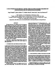
Figure 1: The empirical power functions of the KS test (smooth line) and CvM test (dotted line) for the 4-variate model using 50 × 60-point regular lattice. The simulation is under 10000 runs.

6.0742 and 7.9910 which are approximated by simulation. For ̂ CvM fluctuate ̂ KS and 𝛼 𝜌 = 𝛾 = 𝛿 = 𝜅 = 0 the values of 𝛼 around 0.05 as it should be. This means that, independent of the selected number of the lattice points, both tests attain the specified level of significance. Furthermore, Figure 1 exhibits the graphs of the empirical power function of the KS and CvM tests for 𝛼 = 0.05 associated with hypothesis 𝐻0 specified above against 𝐻1 : 𝑔𝑖 ∉ W𝑖 , for 𝑖 = 1, 2, 3, 4. For the four cases we generate the error vectors independently from the same 4-variate normal distribution mentioned above. In the clockwise direction the left-top panel presents the graphs of the power function for testing 𝐻0 against 𝐻1 : 𝑔1 ∉ W1 , the right-top panel is for 𝐻0 against 𝐻1 : 𝑔2 ∉ W2 , the right-bottom is for 𝐻0 against

𝐻1 : 𝑔3 ∉ W3 , and left-bottom is for 𝐻0 against 𝐻1 : 𝑔4 ∉ W4 . The common characteristic of the tests is that the power gets larger as the the model moves away from 𝐻0 . The KS tests represented by smooth line tend to have slightly larger power. However, somewhat unexpectedly, in the second case, the CvM test has much larger power.

7. Example of Application In this example, the proposed method is applied to a mining data studied in Tahir [20]. As introduced in Section 1, the data consist of a simultaneous measurement of the percentages of Nickel (Ni), Cobalt (Co), Ferum (Fe), and other substances like Calcium-Monoxide (CaO), Silicon-Dioxide (SiO2 ), and

12

International Journal of Mathematics and Mathematical Sciences

Table 2: Pearson’s correlation matrix of the percentages of CaO, log SiO2 , log MgO, Ni, log Fe, and Co observed over a regular lattice of size 7 × 14. Source of data: Tahir [20]. CaO 1.0000 0.3949 0.4045 −0.1285 −0.1166 −0.0665

CaO log SiO2 log MgO Ni log Fe Co

log SiO2 0.3949 1.0000 0.8459 −0.0003 −0.5414 −0.4556

log MgO 0.4045 0.8459 1.0000 −0.1331 −0.4968 −0.3134

Magnesium-Monoxide (MgO). The sample was obtained by drilling bores set according to a three-dimensional lattice of size 7 × 14 × 10 with 7 equidistance rows running west to east, 14 equidistance columns running south to north, and 10 equidistance depths from the surface of the earth to the bottom. To simplify the computation of the test statistics we consider the experimental design as a two-dimensional lattice of size 7 × 14 by taking the average value of the samples measured in the same position. We further assume that the exploration region is given by a closed rectangle so that by suitable rescaling it can be transformed into a closed unit rectangle I2 . Table 2 exhibits, respectively, the pairs scatter plot and Pearson’s correlation coefficient among the percentages of Ni, CaO, Co, the logarithm of the percentages of SiO2 (log SiO2 ), MgO (log MgO), and Fe (log Fe). By this reason a multivariate analysis must be conducted in the statistical modelling taking into account the unknown covariance matrix of the vector of the variables. Furthermore, based on the individual scatter plot of the samples which are not presented in this work, it can be inferred that polynomials of lower order seem to be adequate to approximate the population model. More precisely, let Y fl (𝑌1 , 𝑌2 , 𝑌3 , 𝑌4 , 𝑌5 , 𝑌6 )⊤ be the vector of observations representing the observed percentages of CaO, log SiO2 , log MgO, Co, Ni, and log Fe, respectively. We aim to test the hypothesis 𝐻0 : E (𝑌) 𝛽11 ( ( =( ( (

𝛽21 + 𝛽22 𝑡 + 𝛽23 𝑠

) ) ) , (60) ) )

𝛽31 + 𝛽32 𝑡 + 𝛽33 𝑠 𝛽41 + 𝛽42 𝑡 + 𝛽43 𝑠 𝛽51 + 𝛽52 𝑡 + 𝛽53 𝑠 + 𝛽54 𝑡2 + 𝛽55 𝑡𝑠 + 𝛽56 𝑠2

2 2 (𝛽61 + 𝛽62 𝑡 + 𝛽63 𝑠 + 𝛽64 𝑡 + 𝛽65 𝑡𝑠 + 𝛽66 𝑠 )

0 ≤ 𝑡, 𝑠 ≤ 1, for some unknown constants 𝛽𝑖𝑗 , 𝑖 = 1, 2, 3, 4, 5, 6 and 𝑗 = 1, . . . , 𝑑𝑖 , with 𝑑1 = 1, 𝑑2 = 𝑑3 = 𝑑4 = 3 and 𝑑5 = 𝑑6 = 6. For this case we have W1 fl [𝑓1 ], W2 = W3 = W4 fl [𝑓1 , 𝑓2 , 𝑓3 ], and W5 = W6 fl [𝑓1 , 𝑓2 , 𝑓3 , 𝑓4 , 𝑓5 , 𝑓6 ], with 𝑓1 (𝑡, 𝑠) fl 1, 𝑓2 (𝑡, 𝑠) = 𝑡, 𝑓3 (𝑡, 𝑠) = 𝑠, 𝑓4 (𝑡, 𝑠) = 𝑡2 , 𝑓5 (𝑡, 𝑠) = 𝑡𝑠, and 𝑓6 (𝑡, 𝑠) = 𝑠2 .

Ni −0.1285 −0.0003 −0.1331 1.0000 0.1652 0.1068

log Fe −0.1167 −0.5414 −0.4968 0.1652 1.0000 0.5937

Co −0.0665 −0.4556 −0.3134 0.1068 0.5937 1.0000

We obtained the values KS7×14;A = 1.44109 and CvM7×14;A = 0.936687 with the associated simulated 𝑝 values of 0.98350 and 0.93670, respectively. We notice that in the computation we consider the VCC {[0, 𝑡] × [0, 𝑠] : 0 ≤ 𝑡, 𝑠 ≤ 1} as the index sets instead of A. Hence when using the KS test as well as CvM test the hypothesis will be not rejected for almost all commonly used values of 𝛼. There exists a significant evidence that the assumed model is appropriate for describing the functional relationship between the experimental conditional and the percentages of those elements. In the practice some computational difficulties appear for testing using our proposed method. First, to the knowledge of the authors, the analytical formula for computing the critical and 𝑝 values of the tests have been not yet available in the literatures; therefore we need to approximate them by simulation using computer. Second, although the test procedures are established for a much larger family of sets A, in the application the computation is always restricted to the VCC of subsets of I𝑑 like that of {∏𝑑𝑖=1 [0, 𝑡𝑖 ] ⊂ I𝑑 : 0 < 𝑡𝑖 ≤ 1, 𝑖 = 1, . . . , 𝑑} or {∏𝑑𝑖=1 [𝑠𝑖 , 𝑡𝑖 ] ⊂ I𝑑 : 0 ≤ 𝑠𝑖 < 𝑡𝑖 ≤ 1, 𝑖 = 1, . . . , 𝑑}.

8. Concluding Remark In this article we have developed an asymptotic method for checking the validity of a general multivariate spatial regression model by considering the multidimensional setindexed partial sums of the residuals. For the calibration of the distribution of the test statistics we propose the residual based bootstrap for multivariate regression. It is shown by applying imitation technique that the residual bootstrap resampling technique is consistent. In a simulation study the finite sample size behavior of the KS and CvM statistics is investigated in greater detail. For the first-order model CvM test has much larger power, whereas for constant, secondorder, and third-order models the powers of the two tests are almost the same. Other possibilities of tests for multidimensional case can be obtained by incorporating a sampling technique according to an arbitrary experimental design. Sometimes because of technical, economic, or ecological reason, practitioners will not or cannot sample the observations equidistantly. One possible approach is to sample according to a continuous probability measure; see, for example, the sampling method

International Journal of Mathematics and Mathematical Sciences

13

proposed in Bischoff [11]. Under this concern we get the socalled weighted KS and CvM tests which can be viewed as generalization of the KS and CvM tests studied in this paper. Instead of considering the least squares residuals of the observations we can also define a test by directly investigating the partial sums of the observations. The limit process will be given by a type of signal plus a noise which is given by the multidimensional set-indexed Brownian sheet. Observing the limit process we can formulate likelihood ratio test based on the Cameron-Matrin-Girsanov density formula of the limit process. Establishing such type of test will be of our concern in our future research project.

The variation of 𝜓 over the finite exact cover K is defined by

Appendix

Furthermore, function 𝜓 is said to have bounded variation in the sense of Vitaly on I𝑑 if there exists a real number 𝑀 > 0 such that 𝑉(𝜓; I𝑑 ) ≤ 𝑀 for some real number 𝑀 > 0. The class of such functions is denoted by BVV(I𝑑 ).

A. Function of Bounded Variation on I𝑑 Definition A.1. Let 𝑓 : R𝑑 → R be a real-valued function with 𝑑 variables. For 𝛼𝑘 , 𝛽𝑘 ∈ R, let Δ𝛽𝛼𝑘𝑘 𝑓 be a real-value function defined on R𝑑 , given by Δ𝛽𝛼𝑘𝑘 𝑓 fl 𝑓 (𝑥1 , . . . , 𝑥𝑘−1 , 𝛽𝑘 , 𝑥𝑘+1 , . . . , 𝑥𝑑 ) − 𝑓 (𝑥1 , . . . , 𝑥𝑘−1 , 𝛼𝑘 , 𝑥𝑘+1 , . . . , 𝑥𝑑 ) ,

(A.1)

for 𝑘 = 1, . . . , 𝑑. Furthermore, for 𝛼 fl (𝛼𝑘 )𝑑𝑘=1 and 𝛽 fl (𝛽𝑘 )𝑑𝑘=1 ∈ R𝑑 , Δ𝛽𝛼 𝑓 is defined on R𝑑 recursively starting from the last components of 𝛼 and 𝛽. More precisely, (Δ𝛽𝛼𝑑𝑑 𝑓)) ⋅ ⋅ ⋅) . Δ𝛽𝛼 𝑓 fl Δ𝛽𝛼11 (⋅ ⋅ ⋅ (Δ𝛽𝛼𝑑−1 𝑑−1

(A.2)

Let {𝑗1 , . . . , 𝑗𝑑 } be permutation of {1, 2, . . . , 𝑑}; then it holds that 𝛽𝑗

𝛽

𝛽𝑗

Δ𝛽𝛼 𝑓 = Δ 𝛼𝑗𝑗11 (⋅ ⋅ ⋅ (Δ 𝛼𝑗𝑑−1 (Δ 𝛼𝑗𝑑 𝑓)) ⋅ ⋅ ⋅) 𝑑−1

𝑑

(A.3)

= Δ𝛽𝛼11 (⋅ ⋅ ⋅ (Δ𝛽𝛼𝑑−1 (Δ𝛽𝛼𝑑𝑑 𝑓)) ⋅ ⋅ ⋅) . 𝑑−1 This means that the operation of Δ𝛽𝛼 𝑓 does not depend on Δ𝛽𝛼𝑑𝑑 𝑓 the order. By this reason we write Δ𝛽𝛼 𝑓 by Δ𝛽𝛼11 ⋅ ⋅ ⋅ Δ𝛽𝛼𝑑−1 𝑑−1 ignoring the brackets. The reader is referred to Yeh [33] and Elstrodt [34], pp. 44-45. Definition A.2 (see Yeh [33]). Let Γ𝑘 fl {[𝑥𝑘0 , 𝑥𝑘1 ], [𝑥𝑘1 , 𝑥𝑘2 ], . . . , [𝑥𝑘𝑀 −1 , 𝑥𝑘𝑀 ]} be a collection of 𝑀𝑘 rectangles 𝑘 𝑘 on the unit interval [0, 1] with 0 = 𝑥𝑘0 ≤ 𝑥𝑘1 ≤ ⋅ ⋅ ⋅ ≤ 𝑥𝑘𝑀 = 𝑘

1, for 𝑘 = 1, . . . , 𝑑. The Cartesian product K fl ∏𝑑𝑘=1 Γ𝑘 which consists of 𝑀1 × 𝑀2 × ⋅ ⋅ ⋅ × 𝑀𝑑 rectangles is called a nonoverlapping finite exact cover of I𝑑 . The family of all nonoverlapping finite exact cover of I𝑑 is denoted by J(K). Definition A.3 (see Yeh [33]). For 1 ≤ 𝑤𝑘 ≤ 𝑀𝑘 , with 𝑘 = 1, . . . , 𝑑, let J𝑤1 ⋅⋅⋅𝑤𝑑 be the element of K defined by J𝑤1 ⋅⋅⋅𝑤𝑑 fl ∏𝑑𝑘=1 [𝑥𝑘𝑤 −1 , 𝑥𝑘𝑤 ]. Let 𝜓 : I𝑑 → R be a real-valued function 𝑑

𝑘

𝑘

on I . Operator Δ J𝑤 ⋅⋅⋅𝑤 acting on a function 𝜓 is defined by 1

𝑑

𝑥1

𝑥𝑑𝑤

𝑥2

Δ J𝑤 ⋅⋅⋅𝑤 𝜓 fl Δ 𝑥1𝑤𝑤1 −1 Δ 𝑥2𝑤𝑤2 −1 ⋅ ⋅ ⋅ Δ 𝑥𝑑𝑤𝑑 −1 𝜓. 1

𝑑

1

2

𝑑

(A.4)

𝑀1

𝑀𝑑

1

𝑑

󵄨󵄨 󵄨󵄨 V (𝜓; K) fl ∑ ⋅ ⋅ ⋅ ∑ 󵄨󵄨󵄨Δ J𝑤 ⋅⋅⋅𝑤 𝜓󵄨󵄨󵄨 . 1 𝑑 󵄨 󵄨 𝑤 =1 𝑤 =1

(A.5)

Accordingly, the total variation of 𝜓 over I𝑑 is defined by 𝑉 (𝜓; I𝑑 ) fl

sup V (𝜓; K) .

K∈J(K)

(A.6)

Definition A.4 (see Yeh [33]). Let (𝑥𝑘 )𝑑𝑘=1 be a variable in I𝑑 . For fixed 𝑘, let I𝑘 fl [0, 1]𝑘 be a 𝑘-dimensional unit closed rectangle constructed in the following way. We choose 𝑑 − 𝑘 components of the variable (𝑥𝑘 )𝑑𝑘=1 . For each choice from 𝑑 , we set each 𝑥𝑖 with 0 all possible elements of the set 𝐶𝑑−𝑘 or 1 and let the remaining 𝑘 variables satisfy 0 ≤ 𝑥𝑖 ≤ 1. 𝑑 Then for each 𝑘 we get 2𝑑−𝑘 |𝐶𝑑−𝑘 | unit closed rectangles I𝑘 . 𝑑 For convention we denote the collection of all 2𝑑−𝑘 |𝐶𝑑−𝑘 | of 𝑘 𝑘 𝑘 closed rectangles I by B and the 𝑗th element of B will be denoted by I𝑘𝑗 . Function 𝜓 is said to have bounded variation

in the sense of Hardy on I𝑑 , if and only if for each 𝑘 = 1, . . . , 𝑑 𝑑 and 𝑗 = 1, . . . , 2𝑑−𝑘 |𝐶𝑑−𝑘 | there exists a real number 𝑀𝑗𝑘 > 0 𝑘 such that 𝑉(𝜓I𝑘𝑗 (⋅); I𝑗 ) ≤ 𝑀𝑗𝑘 , where, for 𝑘 = 1, . . . , 𝑑 and 𝑗 =

𝑑 1, . . . , 2𝑑−𝑘 |𝐶𝑑−𝑘 |, 𝜓I𝑘𝑗 (⋅) is a function with 𝑘 variables obtained from the function 𝜓(𝑥1 , 𝑥2 . . . , 𝑥𝑑 ) by setting the 𝑑−𝑘 selected variables with 0 or 1, whereas the remaining 𝑘 variables lie in the interval [0, 1]. The class of such functions will be denoted by BV𝐻(I𝑑 ).

B. Integration by Parts on I𝑑 For family B𝑘 defined in Definition A.4, let I fl ⋃𝑑𝑘=0 B𝑘 , where, for 𝑘 = 0, the family B0 is a collection of 2𝑑 different points in I𝑑 . As an example, for 𝑑 = 2, we have B0 = {I01 = (0, 0), I02 = (0, 1), I03 = (1, 0), I04 = (1, 1)}. For each 𝑘 = 1, . . . , 𝑑 𝑑 |, let ♯(I𝑘𝑗 ) be the number of 1’s and 𝑗 = 1, . . . , 2𝑑−𝑘 |𝐶𝑘−𝑑 appearing in I𝑘𝑗 . Next, let 𝜑 and 𝜓 be defined on I𝑑 . If 𝜑 is Riemann-Stieltjes integrable with respect to 𝜓 on I𝑘𝑗 ∈ B𝑘 , we (𝑅)

denote the integral by ∫I𝑘 𝜑 𝑑𝑘 𝜓. For 𝑘 = 0, it is understood (𝑅)

𝑗

0

that ∫I0 𝜑 𝑑 𝜓 is defined as the product of 𝜑 and 𝜓 at that 𝑗

point of I0𝑗 (see Yeh [33]). Theorem B.1 (integration by parts (see Yeh [33])). Let 𝜑 be Riemann-Stieltjes integrable with respect to 𝜓 on each member

14

International Journal of Mathematics and Mathematical Sciences

of I. Then 𝜓 is Riemann-Stieltjes integrable with respect to 𝜑 on I𝑑 , and we have the formula ∫

(𝑅)

I𝑑

𝜓 (𝑥1 , . . . , 𝑥𝑑 ) 𝑑𝜑 (𝑥1 , . . . , 𝑥𝑑 ) 𝑑−𝑘 𝑑 𝑑 2 |𝐶𝑑−𝑘 |

=∑

∑

𝑘=0

𝑗=1

(𝑅)

𝑘

(−1)(𝑑−♯(I𝑗 )) ∫

I𝑘𝑗

Hence, 𝑉𝑛(𝑖)1 ⋅⋅⋅𝑛𝑑 (𝐴 𝑛1 ⋅⋅⋅𝑛𝑑 ) ∈ H𝐵 having √𝑛1 ⋅ ⋅ ⋅ 𝑛𝑑 𝑠𝐴 𝑛 ⋅⋅⋅𝑛 as the 1

⟨𝑉𝑛(𝑖)1 ⋅⋅⋅𝑛𝑑 (𝐴 𝑛1 ⋅⋅⋅𝑛𝑑 ) , 𝑉𝑛(𝑖)1 ⋅⋅⋅𝑛𝑑 (𝐵𝑛1 ⋅⋅⋅𝑛𝑑 )⟩H

= ∫ √𝑛1 ⋅ ⋅ ⋅ 𝑛𝑑 𝑠𝐴 𝑛 ⋅⋅⋅𝑛 (t) √𝑛1 ⋅ ⋅ ⋅ 𝑛𝑑 𝑠𝐵𝑛 ⋅⋅⋅𝑛 (t) 1 1

𝜑 𝑑𝑘 𝜓.

I𝑑

󵄨󵄨 (𝑅) 󵄨󵄨󵄨 󵄨󵄨 󵄨󵄨∫ 𝜓 (𝑥1 , . . . , 𝑥𝑑 ) 𝑑𝜑 (𝑥1 , . . . , 𝑥𝑑 )󵄨󵄨󵄨 󵄨󵄨󵄨 󵄨󵄨󵄨 I𝑑 𝑑−𝑘 𝑑 𝑑 2 |𝐶𝑑−𝑘 |

𝑘=1

∑

𝑗=1

𝐵

(B.1)

(B.2) 𝑉 (𝜓I𝑘𝑗 (⋅) ; I𝑘𝑗 )) .

𝑑

𝑛1

𝑛𝑑

𝑗1 =1

𝑗𝑑 =1

𝑑

(C.4)

⋅ 𝜆𝑑I (𝑑t) = ∑ ⋅ ⋅ ⋅ ∑ 𝑎𝑗1 ⋅⋅⋅𝑗𝑑 𝑏𝑗1 ⋅⋅⋅𝑗𝑑

Moreover, if 𝜓 have bounded variation in the sense of Hardy on I𝑑 and 𝜑 is continuous on I𝑑 , then we have the inequality

󵄩 󵄩 󵄩 󵄩 ≤ 󵄩󵄩󵄩𝜑󵄩󵄩󵄩∞ (2𝑑 󵄩󵄩󵄩𝜓󵄩󵄩󵄩∞ + ∑

𝑑

𝐿 2 (𝜆𝑑I ) density. By the definition of the inner product ⟨⋅, ⋅⟩H𝐵 , we further get

= ⟨𝐴 𝑛1 ⋅⋅⋅𝑛𝑑 , 𝐵𝑛1 ⋅⋅⋅𝑛𝑑 ⟩R𝑛1 ×⋅⋅⋅×𝑛𝑑 . Lemma C.2 (see Bischoff and Somayasa [9]). For any 𝑛 ,...,𝑛𝑑 in R𝑛1 ×⋅⋅⋅×𝑛𝑑 it holds that, for 𝑖 = 𝐴 𝑛1 ⋅⋅⋅𝑛𝑑 fl (𝑎𝑗1 ⋅⋅⋅𝑗𝑑 )𝑗11=1,...,𝑗 𝑑 =1 1, . . . , 𝑝, 𝑉𝑛(𝑖)1 ⋅⋅⋅𝑛𝑑 (𝑝𝑟W𝑖,𝑛 ⋅⋅⋅𝑛 𝐴 𝑛1 ⋅⋅⋅𝑛𝑑 ) 1

C. Some Property of the Partial Sums Operator

𝑑

= 𝑝𝑟W𝑖,𝑛 ⋅⋅⋅𝑛

𝑑 H𝐵

1

(C.5)

𝑉𝑛(𝑖)1 ⋅⋅⋅𝑛𝑑 (𝐴 𝑛1 ⋅⋅⋅𝑛𝑑 ) ,

where Lemma C.1 (see Bischoff and Somayasa [9]). For every one𝑛 ,...,𝑛𝑑 , dimensional pyramidal array 𝐴 𝑛1 ⋅⋅⋅𝑛𝑑 fl (𝑎𝑗1 ⋅⋅⋅𝑗𝑑 )𝑗11=1,...,𝑗 𝑑 =1

W𝑖,𝑛1 ⋅⋅⋅𝑛𝑑 H fl {𝑉𝑛(𝑖)1 ⋅⋅⋅𝑛𝑑 (𝐵𝑛1 ⋅⋅⋅𝑛𝑑 ) | 𝐵𝑛1 ⋅⋅⋅𝑛𝑑 ∈ W𝑖,𝑛1 ⋅⋅⋅𝑛𝑑 } 𝐵

it holds that ∈ H𝐵 , where H𝐵 is the subspace defined in (15). Furthermore, for any arrays 𝐴 𝑛1 ⋅⋅⋅𝑛𝑑 fl 𝑛 ,...,𝑛𝑑 𝑛 ,...,𝑛𝑑 (𝑎𝑗1 ⋅⋅⋅𝑗𝑑 )𝑗11=1,...,𝑗 and 𝐵𝑛1 ⋅⋅⋅𝑛𝑑 fl (𝑏𝑗1 ⋅⋅⋅𝑗𝑑 )𝑗11=1,...,𝑗 , we have 𝑑 =1 𝑑 =1 ⟨𝑉𝑛(𝑖)1 ⋅⋅⋅𝑛𝑑 (𝐴 𝑛1 ⋅⋅⋅𝑛𝑑 ) , 𝑉𝑛(𝑖)1 ⋅⋅⋅𝑛𝑑 (𝐵𝑛1 ⋅⋅⋅𝑛𝑑 )⟩H

Furthermore, by the definition of the component-wise projection, we finally get V𝑛1 ⋅⋅⋅𝑛𝑑 (𝑝𝑟∏𝑝

𝐵

𝑖=1 W𝑖,𝑛1 ⋅⋅⋅𝑛𝑑

(C.1)

= ⟨𝐴 𝑛1 ⋅⋅⋅𝑛𝑑 , 𝐵𝑛1 ⋅⋅⋅𝑛𝑑 ⟩R𝑛1 ×⋅⋅⋅×𝑛𝑑 ,

= (𝑝𝑟W𝑖,𝑛 ⋅⋅⋅𝑛 1

where 𝑉𝑛(𝑖)1 ⋅⋅⋅𝑛𝑑 is the one-dimensional component of the partial sums operator V𝑛1 ⋅⋅⋅𝑛𝑑 . Proof. Associated with 𝐴 𝑛1 ⋅⋅⋅𝑛𝑑 we can construct a step function 𝑠𝐴 𝑛 ⋅⋅⋅𝑛 : I𝑑 → R defined by 1

𝑑

𝑛1

𝑛𝑑

𝑗1 =1

𝑗𝑑 =1

𝑑

𝑠𝐴 𝑛 ⋅⋅⋅𝑛 (t) fl ∑ ⋅ ⋅ ⋅ ∑ 𝑎𝑗1 ⋅⋅⋅𝑗𝑑 1𝐶𝑗 ⋅⋅⋅𝑗 (t) , t ∈ I , 1

𝑑

1

𝑑

(C.2)

=

1

𝑖=1

(C.7) ,

𝑝

Proof. For fixed 𝑖, let {𝑓𝑖1 (Ξ𝑛1 ⋅⋅⋅𝑛𝑑 ), . . . , 𝑓𝑖𝑑𝑖 (Ξ𝑛1 ⋅⋅⋅𝑛𝑑 )} be an ONB of W𝑖,𝑛1 ⋅⋅⋅𝑛𝑑 . Then by Lemma C.1 the corresponding ONB of W𝑖,𝑛1 ⋅⋅⋅𝑛𝑑 H is given by the set 𝐵

Hence, by the linearity of V(𝑖) 𝑛1 ⋅⋅⋅𝑛𝑑 and by Lemma C.1, we get 𝑉𝑛(𝑖)1 ⋅⋅⋅𝑛𝑑 (prW𝑖,𝑛 ⋅⋅⋅𝑛 𝐴 𝑛1 ⋅⋅⋅𝑛𝑑 ) 1

𝑑

𝑗=1

𝑑

1 𝑉𝑛(𝑖)⋅⋅⋅𝑛 (𝐴 𝑛1 ⋅⋅⋅𝑛𝑑 ) (𝐵) . √𝑛1 ⋅ ⋅ ⋅ 𝑛𝑑 1 𝑑

𝑝

= 𝑉𝑛(𝑖)1 ⋅⋅⋅𝑛𝑑 ( ∑ ⟨𝑓𝑖𝑗 (Ξ𝑛1 ⋅⋅⋅𝑛𝑑 ) , 𝐴 𝑛1 ⋅⋅⋅𝑛𝑑 ⟩R𝑛1 ×⋅⋅⋅×𝑛𝑑

(𝐵) fl ∫ 𝑠𝐴 𝑛 ⋅⋅⋅𝑛 (t) 𝜆𝑑I (𝑑t) 𝐵

𝑉𝑛(𝑖)1 ⋅⋅⋅𝑛𝑑 (𝐴 𝑛1 ⋅⋅⋅𝑛𝑑 ))

for every 𝑝-dimensional array A𝑛1 ⋅⋅⋅𝑛𝑑 ∈ ∏𝑖=1 R𝑛1 ×⋅⋅⋅×𝑛𝑑 .

𝑑𝑖

𝑛1 ⋅⋅⋅𝑛𝑑

𝑑 H𝐵

A𝑛1 ⋅⋅⋅𝑛𝑑 )

(𝑖) {V(𝑖) 𝑛1 ⋅⋅⋅𝑛𝑑 (𝑓𝑖1 (Ξ𝑛1 ⋅⋅⋅𝑛𝑑 )) , . . . , V𝑛1 ⋅⋅⋅𝑛𝑑 (𝑓𝑖𝑑𝑖 (Ξ𝑛1 ⋅⋅⋅𝑛𝑑 ))} . (C.8)

where 𝐶𝑗1 ⋅⋅⋅𝑗𝑑 = ∏𝑑𝑘=1 ((𝑗𝑘 − 1)/𝑛𝑘 , 𝑗𝑘 /𝑛𝑘 ], for 1 ≤ 𝑗𝑘 ≤ 𝑛𝑘 . For any 𝐵 ∈ A, it holds that ℎ𝑠𝐴

(C.6)

⊂ H𝐵 .

V(𝑖) 𝑛1 ⋅⋅⋅𝑛𝑑 (𝐴 𝑛1 ⋅⋅⋅𝑛𝑑 )

(C.3) ⋅ 𝑓𝑖𝑗 (Ξ𝑛1 ⋅⋅⋅𝑛𝑑 ))

International Journal of Mathematics and Mathematical Sciences 𝑑𝑖

Proposition 𝑝𝑟∏𝑝 W𝑖,𝑛 ⋅⋅⋅𝑛

= ∑ ⟨𝑓𝑖𝑗 (Ξ𝑛1 ⋅⋅⋅𝑛𝑑 ) , 𝐴 𝑛1 ⋅⋅⋅𝑛𝑑 ⟩R𝑛1 ×⋅⋅⋅×𝑛𝑑

𝑖=1

𝑗=1

𝑑𝑖

𝑗=1

𝐵

⋅ 𝑉𝑛(𝑖)1 ⋅⋅⋅𝑛𝑑 (𝑓𝑖𝑗 (Ξ𝑛1 ⋅⋅⋅𝑛𝑑 )) 𝑑 H𝐵

𝑉𝑛(𝑖)1 ⋅⋅⋅𝑛𝑑 (𝐴 𝑛1 ⋅⋅⋅𝑛𝑑 ) . (C.9) (𝑛 ⋅⋅⋅𝑛 )

Lemma C.3 (see Bischoff and Somayasa [9]). Let {̃𝑠𝑖1 1 𝑑 , . . . , 1 ⋅⋅⋅𝑛𝑑 ) ̃𝑠(𝑛 } be an orthonormal set in 𝐿 2 (𝜆𝑑I ) obtained by the 𝑖𝑑𝑖 Gram-Schmidt procedure from the step functions: (𝑛 ⋅⋅⋅𝑛𝑑 )

𝑠𝑖𝑗 1

𝑛𝑑

𝑛1

fl ∑ ⋅ ⋅ ⋅ ∑ 𝑓𝑖𝑗 ( 𝑗1 =1

𝑗𝑑 =1

t∈I , for 𝑖 = 1, . . . , 𝑝, and 𝑗 = 1, . . . , 𝑑𝑖 . Then {ℎ̃𝑠(𝑛1 ⋅⋅⋅𝑛𝑑 ) , . . . , ℎ̃𝑠(𝑛1 ⋅⋅⋅𝑛𝑑 ) } is 𝑖1

𝑖𝑑𝑖

an ONB of W𝑖,𝑛1 ⋅⋅⋅𝑛𝑑 H . The projection of any function 𝑢𝑛 ∈ H𝐵 𝐵 into W𝑖,𝑛1 ⋅⋅⋅𝑛𝑑 H with respect to this basis is given by 𝐵

𝑑 H𝐵

𝑢𝑛 = ∑ ⟨ℎ̃𝑠(𝑛1 ⋅⋅⋅𝑛𝑑 ) , 𝑢𝑛 ⟩ 𝑖𝑗

𝑗=1 𝑑𝑖

= ∑∫

𝑝 𝑑𝑖 󵄨 󵄨󵄨 󵄨󵄨 󵄨 󵄨󵄨 = ∑ ∑ 󵄨󵄨󵄨󵄨⟨ℎ̃𝑠(𝑛1 ⋅⋅⋅𝑛𝑑 ) , 𝑤1𝑖 − 𝑤2𝑖 ⟩󵄨󵄨󵄨󵄨 󵄨󵄨󵄨󵄨ℎ̃𝑠(𝑛1 ⋅⋅⋅𝑛𝑑 ) (𝐴)󵄨󵄨󵄨󵄨 𝑖𝑗 󵄨 󵄨 𝑖𝑗 󵄨 𝑖=1 𝑗=1 󵄨

H𝐵

1 ⋅⋅⋅𝑛𝑑 ) ̃𝑠(𝑛 𝑖𝑗

(C.12)

𝑑

ℎ̃𝑠(𝑛1 ⋅⋅⋅𝑛𝑑 ) 𝑖𝑗

(t) 𝑑𝑢 (t) ℎ̃𝑠(𝑛1 ⋅⋅⋅𝑛𝑑 ) . 𝑖𝑗

Moreover, if, for 𝑖 = 1, . . . , 𝑝 and 𝑗 = 1, . . . , 𝑑𝑖 , 𝑓𝑖𝑗 is continuous (𝑛 ⋅⋅⋅𝑛 )

on I𝑑 and {𝑓𝑖1 , . . . , 𝑓𝑖𝑑𝑖 } is an ONB of W𝑖 , then ‖̃𝑠𝑖𝑗 1 𝑑 − 𝑓𝑖𝑗 ‖∞ → 0 as 𝑛1 , . . . , 𝑛𝑑 → ∞. Consequently, it also holds that ‖ℎ̃𝑠(𝑛1 ⋅⋅⋅𝑛𝑑 ) − ℎ𝑓𝑖𝑗 ‖A → 0, for 𝑛1 , . . . , 𝑛𝑑 → ∞. 𝑖𝑗

Proof. Since ℎ𝑠(𝑛1 ⋅⋅⋅𝑛𝑑 ) = (1/√𝑛1 ⋅ ⋅ ⋅ 𝑛𝑑 )𝑉𝑛(𝑖)1 ⋅⋅⋅𝑛𝑑 (𝑓𝑖𝑗 (Ξ𝑛1 ⋅⋅⋅𝑛𝑑 )), by 𝑖𝑗

the linearity of 𝑉𝑛(𝑖)1 ⋅⋅⋅𝑛𝑑 it follows that {ℎ𝑠(𝑛1 ⋅⋅⋅𝑛𝑑 ) , . . . , ℎ𝑠(𝑛1 ⋅⋅⋅𝑛𝑑 ) } 𝑖1

𝑑−𝑘 𝑑 𝑑 2 |𝐶𝑑−𝑘 |

+∑

∑

𝑘=1

ℓ=1

󵄩 󵄩 𝑉 (𝑓𝑖𝑗 𝑘 (⋅) ; I𝑘ℓ )) ≤ 󵄩󵄩󵄩w1 − w2 󵄩󵄩󵄩A 𝐾, I ℓ

for some constant 𝐾 defined by 𝑝

𝑑𝑖

󵄩 󵄩 𝐾 fl ∑ ∑ 󵄩󵄩󵄩󵄩𝑓𝑖𝑗 󵄩󵄩󵄩󵄩∞ 𝑖=1 𝑗=1

𝑑 󵄩 󵄩 ⋅ (2𝑑 󵄩󵄩󵄩󵄩𝑓𝑖𝑗 󵄩󵄩󵄩󵄩∞ + ∑

(C.11) (𝑅)

𝑑 𝑗=1 I

𝑑 | 2𝑑−𝑘 |𝐶𝑑−𝑘

𝑘=1

∑

ℓ=1

(C.13) 𝑉 (𝑓𝑖𝑗 𝑘 (⋅) ; I𝑘ℓ )) . I ℓ

Hence we get 󵄩󵄩 󵄩󵄩 󵄩󵄩pr 𝑝 󵄩 󵄩󵄩 ∏𝑖=1 W𝑖,𝑛1 ⋅⋅⋅𝑛𝑑 H w1 − pr∏𝑝𝑖=1 W𝑖,𝑛1 ⋅⋅⋅𝑛𝑑 H w2 󵄩󵄩󵄩 󵄩 󵄩A 𝐵 𝐵 󵄩 󵄩 ≤ 󵄩󵄩󵄩w1 − w2 󵄩󵄩󵄩A 𝐾.

(C.14)

Given any positive small number 𝜖, there exists a small number 𝛿 fl 𝜀/𝐾, such that, for any w1 , w2 ∈ C𝑝 (A), if ‖w1 − w2 ‖A ≤ 𝛿, then 󵄩󵄩 󵄩󵄩 󵄩󵄩pr 𝑝 󵄩 (C.15) 󵄩󵄩 ∏𝑖=1 W𝑖,𝑛1 ⋅⋅⋅𝑛𝑑 H w1 − pr∏𝑝𝑖=1 W𝑖,𝑛1 ⋅⋅⋅𝑛𝑑 H w2 󵄩󵄩󵄩 ≤ 𝜀. 󵄩 󵄩A 𝐵 𝐵

𝑖𝑑𝑖

builds a basis for W𝑖,𝑛1 ⋅⋅⋅𝑛𝑑 H whenever the set {𝑓𝑖1 (Ξ𝑛1 ⋅⋅⋅𝑛𝑑 ), . . . , 𝐵 𝑓𝑖𝑑𝑖 (Ξ𝑛1 ⋅⋅⋅𝑛𝑑 )} is a basis of W𝑖,𝑛1 ⋅⋅⋅𝑛𝑑 . Furthermore, if 𝑓𝑖𝑗 is (𝑛 ⋅⋅⋅𝑛 )

continuous on I𝑑 , it can be shown that ‖𝑠𝑖𝑗 1 𝑑 − 𝑓𝑖𝑗 ‖∞ → 0 as 𝑛1 , . . . , 𝑛𝑑 → ∞. Hence, by the definition of the GramSchmidt process and also by the continuity of ‖⋅‖𝐿 2 (𝜆𝑑I ) , we can further show that ‖ℎ̃𝑠(𝑛1 ⋅⋅⋅𝑛𝑑 ) − ℎ𝑓𝑖𝑗 ‖A → 0 as 𝑛1 , . . . , 𝑛𝑑 → ∞. 𝑖𝑗

The last assertion is immediately obtained from the definition of ℎ̃𝑠(𝑛1 ⋅⋅⋅𝑛𝑑 ) and ℎ𝑓𝑖𝑗 . 𝑖𝑗

󵄨󵄨 − ⟨ℎ̃𝑠(𝑛1 ⋅⋅⋅𝑛𝑑 ) , 𝑤2𝑖 ⟩ ℎ̃𝑠(𝑛1 ⋅⋅⋅𝑛𝑑 ) (𝐴)󵄨󵄨󵄨󵄨 𝑖𝑗 𝑖𝑗 󵄨

𝑖=1 𝑗=1

(C.10) 𝑑

1

󵄨󵄨 𝑝 𝑑𝑖 󵄨󵄨 ⋅ (𝐴)󵄨󵄨󵄨󵄨 ≤ ∑ ∑ 󵄨󵄨󵄨󵄨⟨ℎ̃𝑠(𝑛1 ⋅⋅⋅𝑛𝑑 ) , 𝑤1𝑖 ⟩ ℎ̃𝑠(𝑛1 ⋅⋅⋅𝑛𝑑 ) (𝐴) 𝑖𝑗 󵄨 𝑖=1 𝑗=1 󵄨 𝑖𝑗

𝑖 󵄩 󵄩 󵄩 󵄩 󵄩 󵄩 ≤ ∑ ∑ 󵄩󵄩󵄩𝑤1𝑖 − 𝑤2𝑖 󵄩󵄩󵄩A 󵄩󵄩󵄩󵄩𝑓𝑖𝑗 󵄩󵄩󵄩󵄩∞ (2𝑑 󵄩󵄩󵄩󵄩𝑓𝑖𝑗 󵄩󵄩󵄩󵄩∞

𝑗1 𝑗 , . . . , 𝑑 ) 1𝐶𝑗 ⋅⋅⋅𝑗 (t) , 1 𝑑 𝑛1 𝑛𝑑

𝑑𝑖

𝑝

Proof. Let w1 fl (𝑤1𝑖 )𝑖=1 and w2 fl (𝑤2𝑖 )𝑖=1 be any functions in C𝑝 (A). Then, by the definition and the inequality presented in Theorem B.1, for any 𝐴 ∈ A we have 󵄨󵄨󵄨 󵄨󵄨(pr∏𝑝 W w1 ) (𝐴) − (pr∏𝑝 W𝑖,𝑛 ⋅⋅⋅𝑛 w2 ) 𝑖,𝑛1 ⋅⋅⋅𝑛𝑑 H 󵄨󵄨 𝑖=1 𝑖=1 1 𝑑 H𝐵 𝐵

𝑝

(t)

𝑝𝑟W𝑖,𝑛 ⋅⋅⋅𝑛

𝑑 H𝐵

𝑝

= ∑ ⟨𝑉𝑛(𝑖)1 ⋅⋅⋅𝑛𝑑 (𝑓𝑖𝑗 (Ξ𝑛1 ⋅⋅⋅𝑛𝑑 )) , 𝑉𝑛(𝑖)1 ⋅⋅⋅𝑛𝑑 (𝐴 𝑛1 ⋅⋅⋅𝑛𝑑 )⟩H

1

1

C.4. The 𝑝-dimensional projection is continuous uniformly on the space of

continuous function C𝑝 (A) for all 𝑛1 ≥ 1, . . . , 𝑛𝑑 ≥ 1.

⋅ 𝑉𝑛(𝑖)1 ⋅⋅⋅𝑛𝑑 (𝑓𝑖𝑗 (Ξ𝑛1 ⋅⋅⋅𝑛𝑑 ))

= prW𝑖,𝑛 ⋅⋅⋅𝑛

15

Competing Interests The authors declare that they have no competing interests.

Acknowledgments The authors wish to thank the Ministry of Research, Technology and Higher Education (RISTEK-DIKTI) for the financial

16 support. They also thank Karlsruher Institut f¨ur Technologie (KIT) Institut f¨ur Stochastik for hospitality. Special thanks are addressed to Professor Andrei I. Volodin for his constructive comments for the improvement of the paper.

References [1] A. Zellner, “An efficient method of estimating seemingly unrelated regressions and tests for aggregation bias,” Journal of the American Statistical Association, vol. 57, no. 298, pp. 348–368, 1962. [2] R. Christensen, Advanced Linear Modeling: Multivariate, Time Series, and Spatial Data; Nonparametric Regression and Response Surface Maximization, Springer, New York, NY, USA, 2001. [3] D. W. Anderson, An Introduction to Multivariate Statistical Analysis, John Wiley & Sons, New York, NY, USA, 3rd edition, 2003. [4] R. A. Johnson and D. W. Wichern, Applied Multivariate Statistical Analysis, Prentice Hall, New York, NY, USA, 3rd edition, 2007. [5] I. B. MacNeill, “Properties of partial sums of polynomial regression residuals with applications to test for change of regression at unknown times,” The Annals of Statistics, vol. 6, no. 2, pp. 422–433, 1978. [6] I. B. MacNeill, “Limit processes for sequences of partial sums of regression residuals,” The Annals of Probability, vol. 6, no. 4, pp. 695–698, 1978. [7] I. B. MacNeill and V. K. Jandhyala, “Change-point methods for spatial data,” in Multivariate Environmental Statistics, G. P. Patil and C. R. Rao, Eds., pp. 298–306, Elevier Science, Berlin, Germany, 1993. [8] L. Xie and I. B. MacNeill, “Spatial residual processes and boundary detection,” South African Statistical Journal, vol. 40, no. 1, pp. 33–53, 2006. [9] W. Bischoff and W. Somayasa, “The limit of the partial sums process of spatial least squares residuals,” Journal of Multivariate Analysis, vol. 100, no. 10, pp. 2167–2177, 2009. [10] W. Somayasa, Ruslan, E. Cahyono, and L. O. Ngkoimani, “Checking adequateness of spatial regressions using setindexed partial sums technique,” Far East Journal of Mathematical Sciences, vol. 96, no. 8, pp. 933–966, 2015. [11] W. Bischoff, “A functional central limit theorem for regression models,” The Annals of Statistics, vol. 26, no. 4, pp. 1398–1410, 1998. [12] W. Bischoff, “The structure of residual partial sums limit processes of linear regression models,” Theory of Stochastic Processes, vol. 2, pp. 23–28, 2002. [13] W. Stute, “Nonparametric model checks for regression,” The Annals of Statistics, vol. 25, no. 2, pp. 613–641, 1997. [14] W. Stute, W. Gonz´alez Manteiga, and M. Presedo Quindimil, “Bootstrap approximations in model checks for regression,” Journal of the American Statistical Association, vol. 93, no. 441, pp. 141–149, 1998. [15] E. J. Bedrick and C.-L. Tsai, “Model selection for multivariate regression in small samples,” Biometrics, vol. 50, no. 1, pp. 226– 231, 1994. [16] Y. Fujikoshi and K. Satoh, “Modified AIC and 𝐶𝑝 in multivariate linear regression,” Biometrika, vol. 84, no. 3, pp. 707–716, 1997. [17] W. Bischoff and A. Gegg, “Partial sum process to check regression models with multiple correlated response: with

International Journal of Mathematics and Mathematical Sciences

[18]

[19] [20]

[21]

[22]

[23]

[24]

[25]

[26] [27]

[28] [29] [30] [31] [32] [33]

[34]

an application for testing a change-point in profile data,” Journal of Multivariate Analysis, vol. 102, no. 2, pp. 281–291, 2011. W. Somayasa and G. N. Adhi Wibawa, “Asymptotic modelcheck for multivariate spatial regression with correlated responses,” Far East Journal of Mathematical Sciences, vol. 98, no. 5, pp. 613–639, 2015. P. Billingsley, Convergence of Probability Measures, John Wiley & Sons, New York, NY, USA, 1968. M. Tahir, “Prediction of the amount of nickel deposit based on the results of drilling bores on several points (case study: south mining region of PT. Aneka Tambang Tbk., Pomalaa, Southeast Sulawesi),” Research Report, Halu Oleo University, Kendari, Indonesia, 2010. K. V. Mardia and C. R. Goodall, “Spatial-temporal analysis of multivariate environmental monitoring data,” in Multivariate Environmental Statistics, G. P. Patil and C. R. Rao, Eds., pp. 347– 386, North-Holland, Amsterdam, The Netherlands, 1993. S. Arnold, “The asymptotic validity of invariant procedures for the repeated measures model and multivariate linear model,” Journal of Multivariate Analysis, vol. 15, no. 3, pp. 325–335, 1984. R. Pyke, “A uniform central limit theorem for partial sum processes indexed by sets,” in London Mathematical Society Lecture Note Series, vol. 79, pp. 219–240, 1983. R. F. Bass and R. Pyke, “Functional law of the iterated logarithm and uniform central limit theorem for partial-sum processes indexed by sets,” The Annals of Probability, vol. 12, no. 1, pp. 13– 34, 1984. K. S. Alexander and R. Pyke, “A uniform central limit theorem for set-indexed partial-sum processes with finite variance,” The Annals of Probability, vol. 14, no. 2, pp. 582–597, 1986. D. W. Stroock, A Concise Introduction to the Theory of Integration, Birkh¨auser, Berlin, Germany, 3rd edition, 1999. J. N. Magnus and H. Neudecker, Matrix Differential Calculus with Applications in Statistics and Econometrics, John Wiley & Sons, New York, NY, USA, 3rd edition, 2007. K. B. Athreya and S. N. Lahiri, Measure Theory and Probability Theory, Springer, New York, NY, USA, 2006. A. W. van der Vaart, Asymptotic Statistics, vol. 3, Cambridge University Press, London, UK, 1998. E. L. Lehmann and J. P. Romano, Testing Statitical Hypotheses, Springer, New York, NY, USA, 3rd edition, 2005. H. Pruscha, Vorlesungen u¨ ber Mathematische Statistik, B.G. Teubner, Stuttgart, Germany, 2000. J. Shao and D. S. Tu, The Jackknife and Bootstrap, Springer, New York, NY, USA, 1995. J. Yeh, “Cameron-Martin translation theorems in the Wiener space of functions of two variables,” Transactions of the American Mathematical Society, vol. 107, no. 3, pp. 409–420, 1963. J. Elstrodt, Maß- und Integrationstheorie, vol. 7 of Korregierte und Aktualisierte Auflage, Springer, Berlin, Germany, 2011.

Advances in

Operations Research Hindawi Publishing Corporation http://www.hindawi.com

Volume 2014

Advances in

Decision Sciences Hindawi Publishing Corporation http://www.hindawi.com

Volume 2014

Journal of

Applied Mathematics

Algebra

Hindawi Publishing Corporation http://www.hindawi.com

Hindawi Publishing Corporation http://www.hindawi.com

Volume 2014

Journal of

Probability and Statistics Volume 2014

The Scientific World Journal Hindawi Publishing Corporation http://www.hindawi.com

Hindawi Publishing Corporation http://www.hindawi.com

Volume 2014

International Journal of

Differential Equations Hindawi Publishing Corporation http://www.hindawi.com

Volume 2014

Volume 2014

Submit your manuscripts at http://www.hindawi.com International Journal of

Advances in

Combinatorics Hindawi Publishing Corporation http://www.hindawi.com

Mathematical Physics Hindawi Publishing Corporation http://www.hindawi.com

Volume 2014

Journal of

Complex Analysis Hindawi Publishing Corporation http://www.hindawi.com

Volume 2014

International Journal of Mathematics and Mathematical Sciences

Mathematical Problems in Engineering

Journal of

Mathematics Hindawi Publishing Corporation http://www.hindawi.com

Volume 2014

Hindawi Publishing Corporation http://www.hindawi.com

Volume 2014

Volume 2014

Hindawi Publishing Corporation http://www.hindawi.com

Volume 2014

Discrete Mathematics

Journal of

Volume 2014

Hindawi Publishing Corporation http://www.hindawi.com

Discrete Dynamics in Nature and Society

Journal of

Function Spaces Hindawi Publishing Corporation http://www.hindawi.com

Abstract and Applied Analysis

Volume 2014

Hindawi Publishing Corporation http://www.hindawi.com

Volume 2014

Hindawi Publishing Corporation http://www.hindawi.com

Volume 2014

International Journal of

Journal of

Stochastic Analysis

Optimization

Hindawi Publishing Corporation http://www.hindawi.com

Hindawi Publishing Corporation http://www.hindawi.com

Volume 2014

Volume 2014