Final Version Submitted to the Theory of Probability and Its Applications, May 1, 2004.
GENERAL ASYMPTOTIC BAYESIAN THEORY OF QUICKEST CHANGE DETECTION
Alexander G. Tartakovsky and Venugopal V. Veeravalli
A BSTRACT. The optimal detection procedure for detecting changes in independent and identically distributed (i.i.d.) sequences in a Bayesian setting was derived by Shiryaev in the nineteen sixties. However, the analysis of the performance of this procedure in terms of the average detection delay and false alarm probability has been an open problem. In this paper, we develop a general asymptotic change-point detection theory that is not limited to a restrictive i.i.d. assumption. In particular, we investigate the performance of the Shiryaev procedure for general discrete-time stochastic models in the asymptotic setting where the false alarm probability approaches zero. We show that the Shiryaev procedure is asymptotically optimal in the general non-i.i.d. case under mild conditions. We also show that the two popular non-Bayesian detection procedures, namely the Page and the Shiryaev-Roberts-Pollak procedures, are generally not optimal (even asymptotically) under the Bayesian criterion. The results of this study are shown to be especially important in studying the asymptotics of decentralized change detection procedures. Keywords and Phrases: Change-point detection, sequential detection, asymptotic optimality, nonlinear renewal theory.
1. Introduction The problem of detecting abrupt changes in stochastic processes arises in a variety of applications including biomedical signal processing, quality control engineering, finance, link failure detection in communication networks, intrusion detection in computer systems, and target detection in surveillance systems [1, 4, 12, 19, 30]. A typical such problem is one of target detection in multisensor systems (radar, infrared, sonar, etc.) [30, 35, 39], where the target appears randomly at an unknown time. The goal is to detect the target as quickly as possible, while maintaining the false alarm rate at a given level. Another application area is intrusion detection in distributed computer networks [4, 12, 39]. Large scale attacks, such as denial-of-service attacks, occur at unknown points in time and need to be detected in the early stages by observing abrupt changes in the network traffic. The design of the quickest change detection procedures usually involves optimizing the tradeoff between two kinds of performance measures, one being a measure of detection delay and the other being a measure of the frequency of false alarms. There are two standard mathematical formulations for the optimum tradeoff problem. The first of these is a minimax formulation proposed by Lorden [17] and Pollak [21], in which the goal is to minimize the worst-case delay subject to a lower bound on the mean time between false alarms. The second is a Bayesian formulation, proposed by Shiryaev [25]-[27], in which the change point is assumed to have a geometric prior distribution, and the goal is to minimize the expected delay subject to an upper bound on false alarm probability. The asymptotic performance of various change-point detection procedures is well understood in the minimax context for both the discrete and continuous-time cases (see [1],[3],[7],[9], [17],[18],[20],[21], [22],[23],[28],[30],[31],[32], [34],[39],[43],[44]). However, there has been little previous work on the asymptotics of Bayesian procedures. The exception is the work by Lai [16] in which the asymptotic properties of Page’s cumulative sum (CUSUM) procedure were studied in a Bayesian (as well as minimax) context for general stochastic models. (See also Beibel [3] for continuous-time Brownian motion and Borovkov [5], Lemma 5 for i.i.d. data models). Our goal is to provide a general Bayesian asymptotic theory for change point detection. The paper is organized as follows. In Section 2, we formulate the problem. In Section 3, we study the behavior of the Shiryaev detection procedure for general, non-i.i.d. data models, and prove that it is asymptotically optimal under mild conditions when the false alarm probability goes to zero. We show that this procedure is asymptotically optimal not only with respect to the average detection delay, but that it is also uniformly asymptotically optimal in the sense of minimizing the conditional expected delay for every change point. Moreover, we study the behavior of higher moments of the detection delay and show that under certain general conditions the Shiryaev procedure minimizes moments of the detection delay up to the given order. In Section 4, we find the asymptotic operating characteristics of the Shiryaev change detection procedure in the i.i.d. case when the false 1
2
A. TARTAKOVSKY AND V. VEERAVALLI
alarm probability goes to zero. The use of nonlinear renewal theory allows us to obtain sharp asymptotic approximations for the false alarm probability and the average detection delay up to vanishing terms. In Section 5, we analyze the asymptotic performance of other well-known change detection procedures (Page’s procedure and the Shiryaev-Roberts-Pollak procedure) in the Bayesian framework. The results of this section allow us to conclude that, while being optimal in the minimax context, these procedures may lose their optimality property (even asymptotically) with respect to the Bayesian criterion depending on the structure of the prior distribution. In Section 6, we consider an example of detecting a change in the mean value of an autoregressive process that illustrates general results. In Section 7, we consider two additional examples related to detecting changes in distributed multi-sensor systems. We study the implications of the asymptotic results in decentralized quickest change detection problems assuming that sensors send quantized versions of their observations to a fusion center (central processor) where the change detection is performed based on all the sensor messages. Finally, in Section 8, we conclude the paper by giving several remarks. The results of this paper have been presented in part at the International Symposium on Information Theory [36] and the Information Theory Workshop [37] in 2002, and at the Sixth International Conference on Information Fusion [38] in 2003. 2. Problem Formulation In the conventional setting of the change-point detection problem one assumes that the observed random variables X1 , X2 , . . . are i.i.d., until a change occurs at an unknown point in time λ, λ ∈ {1, 2, . . . }. After the change occurs, the observations are again i.i.d. but with another distribution. In other words, conditioned on λ = k, the observations X1 , X2 , . . . are independent with Xn ∼ f0 for n < k and Xn ∼ f1 for n > k, where f0 (x) and f1 (x) are, respectively, the pre-change and post-change probability density functions (pdf) with respect to a sigma-finite measure µ. For the sake of brevity, in what follows, this case will be referred to as the “i.i.d. case.” In a Bayesian setting, the change point λ is assumed to be random with prior probability distribution πk = P(λ = k), k = 0, 1, 2, . . . . The goal is to detect the change as soon as possible after it occurs, subject to the false alarm probability constraints. In mathematical terms, a sequential detection procedure is identified with a stopping time τ for an observed sequence {Xn }n>1 , i.e. τ is an extended integer-valued random variable, such that the event {τ 6 n} belongs to the sigma-algebra FnX = σ(X1 , . . . , Xn ). A false alarm is raised whenever the detection is declared before the change occurs, i.e. when τ < λ. A good detection procedure should guarantee a “stochastically small” detection lag τ − λ provided that there is no false alarm (i.e. τ > λ), while the rate of false alarms should be low. Let Pk and Ek denote the probability measure and the corresponding expectation when the change occurs at time λ = k. In what follows, Pπ stands for the “average” probability measure which is defined as Pπ (Ω) = P ∞ π π k=0 πk Pk (Ω), and E denotes the expectation with respect to P . In the Bayesian setting, a reasonable measure of the detection lag is the average detection delay (ADD) ∞
(2.1)
ADD(τ ) = Eπ (τ − λ|τ > λ) =
X Eπ (τ − λ)+ 1 = πk Pk (τ > k)Ek (τ − k|τ > k), Pπ (τ > λ) Pπ (τ > λ) k=0
and the false alarm rate can be measured by the probability of false alarm (2.2)
PFA(τ ) = Pπ (τ < λ) =
∞ X
πk Pk (τ < k).
k=1
x+
Here and henceforth, we use the traditional notation = max(0, x) for the positive part of x. An optimal Bayesian detection procedure is a procedure for which ADD is minimized, while PFA is constrained to be below a given (usually small) level α, α ∈ (0, 1). Specifically, define the class of change-point detection procedures ∆(α) = {τ : PFA(τ ) 6 α} for which the false alarm probability does not exceed the predefined number α. The optimal change-point detection procedure is described by the stopping time ν = arg inf ADD(τ ). τ ∈∆(α)
ASYMPTOTIC THEORY OF QUICKEST CHANGE DETECTION
3
Obviously, if PFA(ν) = α, then ν also minimizes Eπ (τ − λ)+ . Let Xn = (X1 , . . . , Xn ) denote the concatenation of the first n observations, let FnX = σ(Xn ) be a sigmaalgebra generated by Xn , and let pn = P(λ 6 n|FnX ) be the posterior probability that the change occurred before time n. For the i.i.d. case, Shiryaev [25]-[27] proved that if the distribution of the change point is geometric, i.e., P(λ = 0) = π0 , πk = (1 − π0 )ρ(1 − ρ)k−1 , k > 1 (0 < ρ < 1, 0 6 π0 < 1), then the optimal detection procedure is the one that raises an alarm at the first time such that the posterior probability pn exceeds a threshold A, i.e.1 ν(A) = inf {n > 1 : pn > A} ,
(2.3)
where the threshold A = Aα should be chosen so that PFA(ν(A)) = α. A generalization of this result for an arbitrary prior distribution has been stated in Borovkov [5], albeit without proof (see Theorem 8 in [5]). However, except for the case of detecting the change in the drift of the Wiener process observed in continuous time, it is difficult to find a threshold that provides an exact match to the given PFA. Also, there are no results related to the ADD evaluation of this optimal procedure, again, except for the continuous-time Wiener process [27] with exponential prior distribution, and for i.i.d. data models with a geometric prior distribution when ρ → 0 (see Lemma 5 in [5]). While the exact match of the false alarm probability is related to the estimation of the overshoot in the stopping rule (2.3), and for this reason is problematic, a simple upper bound, which ignores overshoot, can be © ª π π obtained. Indeed, since P {ν(A) < λ} = E 1 − pν(A) and 1 − pν(A) 6 1 − A on {ν(A) < ∞}, we obtain that the PFA defined in (2.2) obeys the inequality PFA(ν(A)) 6 1 − A.
(2.4)
It follows that setting A = Aα = 1 − α guarantees the inequality PFA(ν(Aα )) 6 α. Note that inequality (2.4) holds true for arbitrary (proper), not necessarily geometric, prior distributions. More generally, assume that observations are non-i.i.d. in the pre-change and post-change modes. Specifically, let P∞ stand for the probability measure under which the conditional density of Xn given Xn−1 = (X1 , . . . , Xn−1 ) is f0,n (Xn |Xn−1 ) for every n > 1 (i.e. λ = ∞). Furthermore, for any λ = k, 1 6 k < ∞, let Pk stand for the probability measure under which the conditional density of Xn is f0,n (Xn |Xn−1 ) if n 6 k − 1 and is f1,n (Xn |Xn−1 ) if n > k. Therefore, if the change occurs at time λ = k, then the conditional density of the k-th observation changes from f0,k (Xk |Xk−1 ) to f1,k (Xk |Xk−1 ). The log-likelihood ratio (LLR) for the hypotheses that the change occurred at the point λ = k and at λ = ∞ (no change at all) is n
(2.5)
Znk := log
X f1,t (Xt |Xt−1 ) dPk log (Xn ) = , dP∞ f0,t (Xt |Xt−1 )
k 6 n.
t=k
In what follows, we will use the convention that before the observations become available (i.e. for n = 0), Z00 = log[f1,0 (X0 )/f0,0 (X0 )] = 0 almost everywhere. In the rest of the paper, we will consider prior distributions πk = P(λ = k) concentrated on nonnegative integers. The following two classes of prior distributions will be covered: distributions with exponential tail for which log P(λ > k + 1) (2.6) lim = −d, d > 0; k→∞ k and prior distributions with “heavy” tails for which log P(λ > k + 1) = 0. k→∞ k The first class will be denoted by E(d), and the second class by H. Clearly, the geometric prior distribution with the parameter ρ, (2.7)
(2.8)
lim
πk = π0 1l{k=0} + (1 − π0 )ρ(1 − ρ)k−1 1l{k>1} ,
0 < ρ < 1, 0 6 π0 < 1,
1Hereafter we use the convention that inf {∅} = ∞, i.e. ν(A) = ∞ if no such n exists.
4
A. TARTAKOVSKY AND V. VEERAVALLI
belongs to the class E(d) with d = | log(1 − ρ)|. Here and henceforth, 1l{A} denotes an indicator of the set A. Note that a more general case where a fixed d is replaced with the value of dα that depends on α and vanishes when α → 0 can also be handled in a similar way. This more general case has been considered by Lai [16]. However, this slight generalization does not have substantial impact on practical applications. For n > 0, define the likelihood ratio of the hypotheses “H1 : λ 6 n” and “H0 : λ > n” Pn Qn Qk−1 i−1 ) i−1 ) dP(Xn |H1 ) i |X k=0 πk P i=k f1,i (XQ i=1 f0,i (Xi |X , Λn := = ∞ n i−1 ) dP(Xn |H0 ) k=n+1 πk i=1 f0,i (Xi |X where f1,0 (X0 )/f0,0 (X0 ) = 1 almost everywhere by the above convention. Recall that pn = P(λ 6 n|FnX ) denotes the posterior probability of the fact that the change occurred before time n. Write Πn = P(λ > n). It is easily verified that (2.9)
Λn = Λ 0 +
Π−1 n
n X
k
πk eZn
and Λn = pn /(1 − pn ),
n > 1,
k=1
where Λ0 = π0 /(1 − π0 ). Therefore, the Shiryaev stopping rule given in (2.3) can be written in the following form that is more convenient for asymptotic study. (2.10)
νB = inf {n > 1 : Λn > B} ,
B = A/(1 − A),
where B > π0 /(1 − π0 ). Evidently, inequality (2.4) holds in the general, non-i.i.d. case too. Consequently, (2.11)
Bα = (1 − α)/α
implies νBα ∈ ∆(α)
assuming that α < 1 − π0 . It is worth noting that while the Shiryaev procedure (2.10) is optimal in the i.i.d. case (if B is chosen so that PFA(νB ) = α), it may not be optimal in the non-i.i.d. scenario even if we can set the threshold to meet the PFA constraint exactly. In fact, the properties of the Shiryaev procedure in the non-i.i.d. scenario have not been investigated previously. In addition to the Bayesian ADD defined in (2.1), we will also be interested in the behavior of the conditional ADD (CADD) for the fixed change point λ = k, which is defined by CADDk (τ ) = Ek (τ − k|τ > k), k = 1, 2 . . . as well as higher moments of the detection delay Ek {(τ − k)m |τ > k} and Eπ {(τ − λ)m |τ > λ} for m > 1. In the next section, we study the operating characteristics of the Bayesian procedure (2.10) for small PFA (α → 0) in the general, non-i.i.d. case. In Section 4, these results will be specialized to the i.i.d. scenario. 3. Asymptotic Operating Characteristics of the Detection Procedure νB in a Non-i.i.d. Case As we mentioned above, in general, the Shiryaev procedure νB is not optimal even if one is able to chose the threshold B in such a way that PFA(B) = α. However, below we show that this procedure with B = Bα = (1 − α)/α is asymptotically optimal for small PFA under some mild conditions. We will show that in the asymptotic setting, νBα minimizes not only the ADD, but also CADDk for all k > 1. Furthermore, under certain general conditions this procedure minimizes higher moments of the detection delay up to the given order. 3.1. Asymptotic lower bounds for moments of the detection delay. We begin by establishing asymptotic lower bounds for moments of the detection delay, in particular for ADD and CADD of any procedure in the class ∆(α). Later on these bounds will be used to obtain asymptotic optimality results. As we will see, the derivation of the lower bounds is based on the application of the Chebyshev inequality that involves certain probabilities, which are shown to go to 0 when α → 0. We start with the study of the behavior of these probabilities. Let q be a positive finite number and define Lα = Lα (qd ) = | log α|/qd , γε,α (τ ) = Pπ {λ 6 τ < λ + (1 − ε)Lα } , (k) γε,α (τ ) = Pk {k 6 τ < k + (1 − ε)Lα } ,
0 < ε < 1,
ASYMPTOTIC THEORY OF QUICKEST CHANGE DETECTION
5
where qd = q + d in the case of prior distributions with exponential right tail, π ∈ E(d), and qd = q0 = q in the case of heavy-tailed prior distributions π ∈ H. The significance of the number q should be explained in more detail. We do not assume any particular model for the observations, and as a result, there is no “structure” of the LLR process. We hence have to impose some conditions on the behavior of the LLR process at least for large n. It is natural to assume that there exists a positive finite number q = q(f1 , f0 ) such that Znk /(n − k) converges almost surely to q, i.e. 1 k P −a.s. Zk+n −−k−−→ q for every k < ∞. n→∞ n This is always true for i.i.d. data models, in which case q = D(f1 , f0 ) = E1 Z11 is the Kullback-Leibler information number. It turns out that the a.s. convergence condition (3.1) is sufficient for obtaining lower bounds for all positive moments of the detection delay (but not necessary). In fact, the key condition (3.2) in Lemma 1 and Theorem 1 holds whenever Znk /(n − k) converges almost surely to the number q. Therefore, this number is of paramount importance in the general change-point detection theory. X , P (τ < k) = P (τ < k), and hence, Note that, since {τ < k} belongs to the sigma-field Fk−1 ∞ k
(3.1)
PFA(τ ) =
∞ X
πk P∞ (τ < k).
k=1
The following “fundamental” lemma will be repeatedly used to derive lower bounds for the performance indices. L EMMA 1. Let Znk be defined as in (2.5) and assume that for some q > 0 ½ ¾ 1 k max Z > (1 + ε)q −−−−→ 0 for all ε > 0 and k > 1. (3.2) Pk M →∞ M 06n 1, (k) lim sup γε,α (τ ) = 0,
(3.3)
α→0 τ ∈∆(α)
and for all 0 < ε < 1, (3.4)
lim sup γε,α (τ ) = 0.
α→0 τ ∈∆(α)
P ROOF. Changing the measure P∞ → Pk , we obtain that for any C > 0 and ε ∈ (0, 1) n o k P∞ {k 6 τ < k + (1 − ε)Lα } = Ek 1l{k6τ Ek 1l{k6τ 1 : max (Πn ) πk > B , B > π0 /(1 − π0 ). 06k6n f0,i (Xi |Xi−1 ) i=k
If B = Bα = (1 − α)/α, then τBα ∈ ∆(α) and Theorems 3–4 hold true for τBα . 6. Example 1: Change Detection in the Mean of the Autoregressive Process In this section, we consider an example that illustrates the results of the previous sections. This example is focussed on single-sensor or centralized detection. In the next section, we will consider two more examples that are related to decentralized (distributed) detection in multi-sensor systems. In the rest of the paper, without special emphasis the prior distribution will be assumed geometric (2.8) with π0 = 0. Consider the “signal plus noise” model, in which we assume that Xn = 1l{n>λ} θn + ξn , n > 1, where θn is a deterministic signal that appears at an unknown point in time λ, and {ξn , n > 1} is a Markov Gaussian sequence (noise), which obeys the recursion ξn = δξn−1 + wn ,
n > 1,
ξ0 = 0.
Here w1 , w2 , . . . are i.i.d. Gaussian random variables with mean zero and variance σ 2 . The parameters 0©6 δ < 1ª and σ > 0 are assumed to be known (δ is the correlation coefficient of noise). Let ϕ(x) = (2π)−1/2 exp −x2 /2 denote the pdf of the standard normal distribution.
22
A. TARTAKOVSKY AND V. VEERAVALLI
For this model, the conditional pdfs f0,n (Xn |Xn−1 ) and f1,n (Xn |Xn−1 ) introduced in Section 2 are of the form ´ ³ n−1 f0,n (Xn | Xn−1 ) = f0 (Xn | Xn−1 ) = σ1 ϕ Xn −δX for all n > 1, σ ³ ´ for n = λ, f1,n (Xn | Xn−1 ) = f1,n (Xn | Xn−1 ) = σ1 ϕ Xn −δXσn−1 −θn ´ ³ n −δθn−1 ) f1,n (Xn | Xn−1 ) = f1,n (Xn | Xn−1 ) = σ1 ϕ Xn −δXn−1 −(θ for n > λ + 1, σ where X0 = θ0 = 0. ei = Xi − δXi−1 and θ˜i = θi − δθi−1 . It is easy to see that Write X Ã ! Ã ! n n X X 1 1 k 2 2 ek + ei − Zn = 2 θk X θk + θ˜i X θ˜i , σ 2σ 2 i=k+1
1 6 k 6 n.
i=k+1
en , n = 1, 2, . . . are independent normal random Next, obviously, conditioned on the change point λ = k, X 2 e e en = θ˜n for n > variables with variance σ , and Ek Xn = 0 for n < k, Ek Xn = θn for n = k, and Ek X k k. Therefore, conditioned on λ = k, {Zn , n > k} is a Gaussian process with independent increments and parameters à ! n X 1 2 k k 2 Ek Zn = −E∞ Zn = 2 θk + θ˜i , 2σ i=k+1 ! à n X 1 θ˜i2 . Vark (Znk ) = Var∞ (Znk ) = 2 θk2 + σ i=k+1
Write Qk,n
k+n−1 1 X ˜2 θi = 2 σ n i=k
and assume that lim Qk,n = Q for all k > 1,
(6.1)
n→∞
where Q characterizes the average “signal-to-noise ratio”, 0 < Q < ∞. It is easily verified that ( √ ) ¯ n¯ o (ε − ∆k,n ) n ¯ k ¯ p Pk ¯Zk+n−1 − Qn/2¯ > εn = 2Φ − , Qk,n where Φ(x) is the standard normal distribution function and ∆k,n = (Qk,n − Q)/2. By condition (6.1), ∞ ¯ n¯ o X ¯ k ¯ nr−1 Pk ¯Zk+n−1 − Qn/2¯ > εn < ∞ for all r > 0, n=1
and hence, for all r > 0 Pk −r−quickly
k n−1 Zk+n −−−−−−−−→ n→∞
Q 2
P∞ −r−quickly
k and n−1 Zk+n −−−−−−−−−→ − n→∞
Q . 2
Thus, condition (3.25) holds for all positive r. Also, evidently, ! Ã∞ ∞ ¯ o n¯ X X ¯ ¯ k − Qn/2¯ > εn < ∞, πk nr−1 Pk ¯Zk+n−1 k=1
n=1
which implies condition (3.26). Thus, under condition (6.1) with 0 < Q < ∞, according to Theorem 3, the Shiryaev detection algorithm νB with B = (1 − α)/α asymptotically minimizes all positive moments of the detection delay in the class ∆(α), and the asymptotic formulas (3.44) and(3.45) hold with q = Q/2.
ASYMPTOTIC THEORY OF QUICKEST CHANGE DETECTION
23
This result can be easily generalized for the problem of detecting a change in the mean of the p-th order Gaussian autoregressive process ξn =
p X
δj ξn−j + wn ,
n > 1,
ξk = 0 for k 6 0,
j=1
where wn , n > 1 are i.i.d. N (0, σ 2 ). Specifically, define θ˜p,n = θn − n X 1 2 θ˜p,k = Q, n→∞ σ 2 (n − p)
lim
Pp
j=1 θn−j
and assume that
where 0 < Q < ∞.
k=p+1
Then Theorem 3 and Corollary 1 show that νB is asymptotically optimal, and asymptotic formulas (3.44)–(3.47) hold true with q = Q/2. We now return to the Markov case and assume that the mean value is constant, θn = θ 6= 0. Then condition (6.1) is fulfilled with Q = θ2 (1 − δ)2 /σ 2 . In the latter case, the results of Subsection 4.2 can be applied. To show this, we first note that the LLR Zn1 can be written in the form n X θ θ2 1 Zn = ∆Wn + 2 X1 − 2 , σ 2σ k=2
where θ(1 − δ) e θ2 (1 − δ)2 X − , k σ2 2σ 2 are i.i.d. Gaussian random variables with parameters ∆Wk =
(6.2)
E1 ∆Wk = −E∞ ∆Wk = Q/2,
k > 2,
Var1 (∆Wk ) = Var∞ (∆Wk ) = Q.
Therefore, by adding and subtracting the random variable ∆W1 , which has the same distribution as ∆W2 , ∆W3 , . . . , one can represent Zn1 in the form Zn1 = Wn + S with Wn = ∆W1 + · · · + ∆Wn being a Gaussian random walk with the parameters given by (6.2), and S = θ θ2 X − 2σ 2 − ∆W1 being a Gaussian random variable with E1 S = −E∞ S = QAδ /2, where Aδ = [1 − (1 − σ2 1 2 δ) ]/(1 − δ)2 . In further calculations, including Monte Carlo experiments, the stopping time νB will be defined as νB = inf{n > 1 : Rρ,n > B} with Rρ,n = Λn /ρ. A slight modification of the proof of Theorem 5 shows that the PFA obeys the asymptotic formula (4.18) and, as B → ∞, (6.3)
E1 νB =
£ ¤ 1 log B − C(ρ, Q) + κ(ρ, Q) − QAδ /2 + o(1). Q/2 + | log(1 − ρ)|
As compared to the asymptotic expansion (4.19) for the i.i.d. case, here an additional term −QAδ /2 appears due to the random variable S in the decomposition of the LLR. To guarantee the given PFA α in simulations, we used the following threshold value obtained by reverting to (4.18) in Theorem 5, (6.4)
B = ζ(ρ, Q)/(αρ).
According to Corollary 2.2.7 of Woodroofe [42], the constant ζ(ρ, Q) is computed from the formula ( ∞ ) X1 2 (6.5) ζ(ρ, Q) = exp − Fk (ρ, Q) , Q + 2| log(1 − ρ)| k k=1
24
where
(6.6)
A. TARTAKOVSKY AND V. VEERAVALLI
µ ¶ Q + 2| log(1 − ρ)| √ √ Fk (ρ, Q) = Φ − k 2 Q µ ¶ Q − 2| log(1 − ρ)| √ k √ + (1 − ρ) Φ − k 2 Q
Rx and Φ(x) = −∞ ϕ(t)dt is a standard normal distribution function. To compute the CADD, we used the following higher order approximation n ³ (6.7) CADD1 (νB ) ≈ max 0, Q2ρ log B − C(ρ, Q) + κ(ρ, Q) −
QAδ 2
´
o −1 ,
where, according to Corollary 2.2.7 of Woodroofe [42], Ã " Ã √ ! √ !# ∞ Q2ρ /4 + Q p X Qρ Qρ k Qρ k −1/2 √ κ(ρ, Q) = − Q − √ Φ − √ . k ϕ Qρ 2 Q 2 Q 2 Q k=1
Here we used the notation Qρ = Q + 2| log(1 − ρ)|. Formula (6.7) follows from the higher order (HO) asymptotic (6.3). Note that this formula requires the computation of the constant C(ρ, Q) using (4.15). As we observed in Remark 4, we usually have to resort to Monte Carlo methods to estimate C(ρ, Q). Values of C for various choices of Q, ρ and δ are given in Table 1. The number of trials were such that the estimate of the standard deviation of C was within 0.5% of the mean. For the purpose of comparison, we also used the first order (FO) approximations for CADD (see (3.29)) ½ ¾ 2 log B (6.8) CADD1 (νB ) ≈ max 0, −1 . Q + 2| log(1 − ρ)| Extensive Monte Carlo simulations have been performed for different values of Q, ρ, δ, and α. The number of trials used for these results is given by 1000/α. Sample results are shown in Tables 2, 3 and 4. In these tables, we present the Monte Carlo (MC) estimates of ADD along with the theoretical values computed according to (6.7) and (6.8). The abbreviations MCADD, MCCADD1 , FOADD, and HOCADD1 are used for the ADD obtained by the MC experiment, CADD1 obtained by the MC experiment, the FO approximation (6.8), and the HO approximation (6.7) for CADD1 , respectively. We also list MC estimates for the false alarm probability PFA. TABLE 1. Values of the constant C for different Q, ρ, δ δ Q 1.0 1.0 1.0 1.0 0.5 0.5 0.5 0.5 0.25 0.25 0.25 0.25 0.1 0.1 0.1 0.1
= 0 (i.i.d.) ρ C 0.3 0.8366 0.1 1.2396 0.03 1.4036 0.01 1.4647 0.3 0.9949 0.1 1.5859 0.03 1.9001 0.01 2.0371 0.3 1.0913 0.1 1.8694 0.03 2.3827 0.01 2.5992 0.3 1.1630 0.1 2.1290 0.03 2.9164 0.01 3.3528
Q 1.0 1.0 1.0 1.0 0.5 0.5 0.5 0.5 0.25 0.25 0.25 0.25 0.1 0.1 0.1 0.1
δ = 0.5 ρ C 0.3 0.5062 0.1 0.7538 0.03 0.8681 0.01 0.9081 0.3 0.7590 0.1 1.2211 0.03 1.5002 0.01 1.5936 0.3 0.9479 0.1 1.6444 0.03 2.1245 0.01 2.3196 0.3 1.0970 0.1 2.0009 0.03 2.7597 0.01 3.1722
ASYMPTOTIC THEORY OF QUICKEST CHANGE DETECTION
25
TABLE 2. Results for i.i.d. case with B = (1 − α)/(ρα) ρ = 0.1, Q = 0.25 α MCPFA MCADD MCCADD1 0.1000 0.0768 9.2315 12.3424 0.0600 0.0464 11.1187 14.4889 0.0300 0.0215 14.0684 17.6605 0.0100 0.0070 18.7026 22.4509 0.0060 0.0043 20.8690 24.6155 0.0030 0.0024 23.7940 27.6285 0.0010 0.0007 28.5247 32.3746 ρ = 0.1, Q = 0.1 α MCPFA MCADD MCCADD1 0.1000 0.0858 11.9405 16.4280 0.0600 0.0460 14.7162 19.7314 0.0300 0.0240 18.9581 24.2873 0.0100 0.0083 25.6559 31.3594 0.0060 0.0048 28.8515 34.6259 0.0030 0.0025 33.2216 39.0867 0.0010 0.0008 40.2447 46.1591
FOADD HOCADD1 18.5338 11.9508 20.9400 14.4484 24.0854 17.5509 28.9431 22.3195 31.1781 24.6034 34.2001 27.5586 38.9779 32.3523 FOADD HOCADD1 27.9637 15.8823 31.5316 19.4116 36.1953 24.0955 43.3981 31.2017 46.7120 34.5589 51.1929 39.0017 58.2772 46.1774
Table 2 contains results of analysis in the i.i.d. case when the threshold B = (1 − α)/(ρα). This threshold value is based on the general upper bound that ignores the overshoot. It can be seen that the MC estimates for PFA in this case are substantially smaller than the design values α. This leads to an increase of the true values of the average detection delay, which is undesirable. It can also be seen that FO approximations are inaccurate even for relatively small α, while HO approximations are very accurate. The results in Table 3 correspond to the i.i.d. case where the threshold B is set using (6.4). It is seen that the MC estimates for PFA match α very closely, especially for values smaller than 0.01. Thus, (6.4) provides an accurate method to design the threshold B to meet the PFA constraint α. It is also seen that, as expected, MCCADD1 exceeds MCADD in all cases. The FOADD values are not good approximations even when PFA is small. On the other hand, the higher order approximation for CADD1 (given by HOCADD1 ) is seen to be very accurate even for moderate values of PFA. Results for the correlated case with δ = 0.5 are presented in Table 4, with the threshold B being set using (6.4). Here again we see the accuracy of our higher order approximations for PFA and ADD. Also, it is interesting to see that for the same value of effective signal-to-noise ratio, Q, the ADD in the correlated case is slightly smaller than in the i.i.d. case. On the other hand, if we fix the value of “actual” signal-to-noise ratio θ2 /σ 2 , e.g., Q = 1 in the i.i.d. case and Q = 0.25 in the δ = 0.5 case, then we can see that the correlation slows down the change detection. 7. More Examples: Decentralized Quickest Change Detection The results of the previous sections are particularly useful in analysis of the decentralized version of the change detection problem described in [41]. We first outline this interesting problem and related asymptotic optimality results for i.i.d. data models. Then we give two examples. 7.1. A decentralized detection problem. Assume that the information about the change is available through a set of L separate sensors. At time n an observation X`,n is made at sensor S` . Conditioned on the change point λ, the observation sequences {X1,n }, {X2,n }, . . . , {XL,n } are assumed to be mutually independent. Furthermore, throughout this section, we restrict our attention to the “i.i.d. case” where the observations in a particular (0) sequence, say {X`,n }n>1 , are independent conditioned on λ, have a common pdf f` before the change, and a (1) common pdf f` from the time of change. Note that we are assuming that all the sensors change distribution at
26
A. TARTAKOVSKY AND V. VEERAVALLI
TABLE 3. Results for i.i.d. case with B = ζ(ρ, Q)/(ρα) α MCPFA 0.1000 0.0914 0.0600 0.0554 0.0300 0.0293 0.0100 0.0100 0.0060 0.0059 0.0030 0.0030 0.0010 0.0010 α MCPFA 0.1000 0.0907 0.0600 0.0547 0.0300 0.0290 0.0100 0.0100 0.0060 0.0058 0.0030 0.0030 0.0010 0.0010 α MCPFA 0.1000 0.0915 0.0600 0.0558 0.0300 0.0284 0.0100 0.0096 0.0060 0.0060 0.0030 0.0029 0.0010 0.0010 α MCPFA 0.1000 0.0914 0.0600 0.0549 0.0300 0.0298 0.0100 0.0097 0.0060 0.0060 0.0030 0.0030 0.0010 0.0010
ρ = 0.1, Q = 1 MCADD MCCADD1 3.9388 4.9192 4.6407 5.7084 5.7191 6.8523 7.4474 8.6344 8.2627 9.4719 9.3973 10.6116 11.1895 12.4177 ρ = 0.01, Q = 1 MCADD MCCADD1 8.5173 9.9681 9.5119 11.0090 10.7933 12.2914 12.9459 14.4763 13.9602 15.4800 15.2986 16.8320 17.4523 18.9875 ρ = 0.1, Q = 0.25 MCADD MCCADD1 8.4385 11.4574 10.2942 13.5159 12.9266 16.3797 17.4060 21.0897 19.4797 23.2396 22.4640 26.2587 27.1694 31.0175 ρ = 0.1, Q = 0.1 MCADD MCCADD1 11.3236 15.7955 13.8997 18.8115 17.8510 23.1455 24.3888 30.0665 27.5188 33.2905 31.9391 37.7784 38.9244 44.8407
FOADD HOCADD1 5.6139 4.8214 6.4577 5.6622 7.6027 6.8195 9.4175 8.6221 10.2614 9.4494 11.4064 10.6225 13.2212 12.4328 FOADD HOCADD1 11.4037 9.9424 12.4052 10.9459 13.7642 12.3139 15.9181 14.4788 16.9196 15.4538 18.2786 16.8507 20.4325 18.9818 FOADD HOCADD1 17.6206 11.0010 19.8381 13.2243 22.8471 16.2042 27.6162 21.0265 29.8337 23.2110 32.8426 26.2497 37.6117 31.0254 FOADD HOCADD1 27.2882 15.1322 30.5762 18.3927 35.0377 22.8742 42.1091 29.9915 45.3971 33.1729 49.8586 37.7489 56.9300 44.8114
the change time λ. As in Section 4, we will suppose that the prior distribution is geometric with the parameter ρ, ρ > 0. Based on the information available at S` at time n, a message U`,n , belonging to a finite alphabet of size V` , is formed and sent to the fusion center. We will use the vector notation: Xn = (X1,n , X2,n , . . . , XL,n ) and Un = (U1,n , U2,n , . . . , UL,n ). Based on the sequence of sensor messages, a decision about the change is made at the fusion center. The fusion center picks a time τ , which is a stopping time on {Un }n>1 , at which it is declared that a change has occurred. Various information structures are possible for the decentralized configuration depending on how feedback and local information is used at the sensors [41]. Consider the simplest information structure where the message U`,n formed by sensor S` at time n is a function of only its current observation X`,n , i.e., Un,` = ψ`,n (X`,n ).
ASYMPTOTIC THEORY OF QUICKEST CHANGE DETECTION
27
TABLE 4. Results for correlated case with δ = 0.5 ρ = 0.1, Q = 1 α MCPFA MCADD MCCADD1 0.1000 0.0839 2.9519 3.3721 0.0600 0.0532 3.5588 4.0728 0.0300 0.0289 4.5526 5.1437 0.0100 0.0100 6.2505 6.9137 0.0060 0.0062 7.0655 7.7425 0.0030 0.0029 8.1902 8.8830 0.0010 0.0010 9.9847 10.6885 ρ = 0.1, Q = 0.25 α MCPFA MCADD MCCADD1 0.1000 0.0895 7.8914 10.6258 0.0600 0.0568 9.7496 12.7327 0.0300 0.0289 12.3524 15.5596 0.0100 0.0098 16.7599 20.2234 0.0060 0.0061 18.8899 22.4150 0.0030 0.0030 21.8352 25.3999 0.0010 0.0010 26.5485 30.1661
FOADD HOCADD1 5.6139 3.1324 6.4577 3.9739 7.6027 5.1293 9.4175 6.9328 10.2614 7.7790 11.4064 8.9244 13.2212 10.7444 FOADD HOCADD1 17.6206 10.3019 19.8381 12.6246 22.8471 15.6679 27.6162 20.3995 29.8337 22.5276 32.8426 25.6374 37.6117 30.4034
Moreover, since for a particular `, the sequence {X`,n }n>1 is assumed to be i.i.d., it is natural to confine ourselves to stationary quantizers2 for which the quantizing functions ψ`,n do not depend on n, i.e. ψ`,n = ψ` for all n > 1. The set of quantizing functions {ψ` , ` = 1, . . . , L} = Ψ, together with the fusion center stopping time τ , form a policy φ = (τ, Ψ). The goal is to choose the policy φ that minimizes the ADD(φ) = Eπ {τ − λ|τ > λ}, or more generally the moments of the detection delay EDπm (φ) = Eπ {(τ − λ)m |τ > λ} for all m > 1, while maintaining the false alarm probability PFA(φ) = Pπ {τ < λ} at a level not greater than α. Let Hk be the hypothesis that the change occurs at time λ = k ∈ {1, 2, . . . }, and let H∞ be the hypothesis that the change does not occur at all. Since the observations at each sensor S` , {X`,n , n = 1, 2, . . .}, are i.i.d., (j) for stationary sensor quantizers, the sensor outputs, {U`,n , n = 1, 2, . . .} will also be i.i.d. Let g` denote the (j) pmf (probability mass function) induced on U`,n when the observation X`,n is distributed as f` , j = 0, 1. Then, for fixed stationary sensor quantizers, the LLRs between the hypotheses Hk and H∞ at the sensor S` and at the fusion center are given by Znk (`) =
n X i=k
(1)
log
g` (U`,i ) (0) g` (U`,i )
and Znk =
L X
Znk (`).
`=1
For fixed sensor quantizers, the fusion center faces a standard change-point detection problem based on the vector observation sequence {Un }. Hence we can define the average likelihood ratio statistic Λdc n and the QL (1) (0) dc dc corresponding statistic Rρ,n = Λn /ρ with f1 (Xn )/f0 (Xn ) now replaced by `=1 [g` (U`,n )/g` (U`,n )]. The index “dc” will be used to denote parameters associated with the decentralized detection problem. dc is given by The decentralized Shiryaev detection procedure at the fusion center νB n o dc dc (7.1) νB = inf n > 1 : Rρ,n >B , where B is a positive threshold which is selected so that PFA(νB ) 6 α. (1) (0) (1) (0) If D(g` , g` ), the K-L distances between the g` and g` , are positive and finite, then for fixed stationary dc given in (7.1), with sensor quantizers, an application of Theorem 4 gives us that the detection procedure νB 2We can prove the optimality of stationary quantizers under some mild conditions on the observations and the quantizers.
28
A. TARTAKOVSKY AND V. VEERAVALLI
B = Bα = (1 − α)/(αρ), is asymptotically optimal as α → 0 among all procedures with PFA no greater than α. To be specific, let Ψ = {ψ1 , . . . , ψL } be a set of stationary quantizers. Then, as α → 0, for all m > 1 !m à | log α| dc inf EDπm (Ψ, τ ) ∼ EDπm (Ψ, νB , )∼ P α (1) (0) L τ ∈∆(α) `=1 D(g` , g` ) + | log(1 − ρ)| where EDπm (Ψ, τ ) = Eπ {(τ − λ)m |τ > λ} is the m−th moment of the detection delay for the policy (Ψ, τ ). This result immediately reveals how to optimize the sensor quantizers. C OROLLARY 3. It is asymptotically optimum (as α → 0) for sensor S` to use the stationary quantizer that (1) (0) maximizes the K-L information distance at its output, i.e., ψ`,opt = Arg Max D(g` , g` ), ` = 1, . . . , L. Based on the results of Tsitsiklis [40], it is easy to show that the optimum stationary quantizer ψ`,opt is a monotone likelihood ratio quantizer (MLRQ), i.e. there exist thresholds h`,1 , h`,2 , . . . , h`,V` −1 satisfying 0 = h`,0 6 h`,1 6 h`,2 6 · · · 6 h`,V` −1 6 ∞ = h`,V` such that (1)
ψ`,opt (X) = i only if h`,i−1
1 at the fusion center (as described in (7.1)). (1) (0) For each `, let the pmfs induced on U`,n by the optimum MLRQ ψ`,opt be given by g`,opt and g`,opt . Then the effective K-L information distance between the “change” and “no change” hypotheses at the fusion center is given by Dtot =
L X
(1)
(0)
D(g`,opt , g`,opt ).
`=1 dc νopt
Finally, denote by Shiryaev’s stopping rule at the fusion center for the case where the sensor quantizers are chosen to be ψ`,opt , and by Φst (α) the class of policies φ with all stationary quantizers and stopping rules at the fusion center such that τ ∈ ∆(α). The asymptotic performance of the asymptotically optimum solution to the decentralized change detection problem described above is given in the following theorem, which follows directly from Theorem 4 and the argument given above. T HEOREM 7. Suppose that (1)
(0)
0 < D(g`,opt , g`,opt ) < ∞ for ` = 1, . . . , L. dc ) 6 α and for all m > 1 Then Bα = (1 − α)/(αρ) implies that PFA(νopt µ ¶m | log α| π π inf EDm (φ) ∼ EDm (φopt ) ∼ Dtot + | log(1 − ρ)| φ∈Φst (α)
as α → 0,
dc , {ψ where φopt = (νopt `,opt }).
Theorem 5 can also be applied to the problem in question. Specifically, if in addition to conditions of TheP (1) (0) orem 7, we assume that the LLR at the fusion center Z11 = L `=1 log[g`,opt (U`,1 )/g`,opt (U`,1 )] is nonarithmetic, then the false alarm probability satisfies asymptotic formula (4.18) with B replaced by Bρ and (7.2)
E1 νB =
£ ¤ 1 log B − C(ρ, Dtot ) + κ(ρ, Dtot ) + o(1) Dtot + | log(1 − ρ)|
with the corresponding modification of the definitions of κ(ρ, Dtot ) and C(ρ, Dtot ).
ASYMPTOTIC THEORY OF QUICKEST CHANGE DETECTION
29
7.2. Example 2: Decentralized detection of a change in the mean of a normal population. Surveillance systems, such as those used in defense, deal with the detection and tracking of moving targets that appear and disappear at unknown points in time. As a result, the target detection problem can be naturally formulated as a multi-sensor abrupt change detection problem considered in Section 7.1. We now consider an example that is of interest in target detection theory. In the centralized setting, this example is a particular case of Example 1. Here we consider the decentralized problem discussed above. Consider the problem of detecting a non-fluctuating target using L geographically separated sensors. The observations are corrupted by additive white Gaussian noise that is independent from sensor to sensor. The sensors preprocess the observations using a matched filter, matched to the signal corresponding to the target (see Poor [24]). The output of the matched filter at sensor S` at time n (when the time of appearance of the target is λ) is given by: ( ξ`,n if n < λ X`,n = µ` + ξ`,n if n > λ, where {ξ`,n , n = 1, 2, . . .} is a sequence of i.i.d. zero-mean Gaussian random variables with variance σ`2 . Therefore, the likelihood ratio at sensor S` is given by ½ ¾ (1) f` (x) µ` (x − µ` /2) (7.3) Y` (x) = (0) = exp . σ`2 f (x) `
Since Y` is monotonically increasing, we can characterize the optimum stationary sensor quantizers in terms of thresholds on the observations, rather than on their likelihood ratios. To further simplify the example, we assume that the sensor messages are binary, i.e., V` = 2 for all `. Then the quantizers reduce to binary tests that are characterized by a single threshold, i.e. ( 1 if X`,n > h` U`,n = 0 otherwise. The distributions induced on U`,n by this quantizer are given by: µ ¶ h` − jµ` (j) (j) (j) (7.4) g` (0) = 1 − g` (1) = Φ = q` , j = 0, 1, σ` where Φ(·) is the distribution function of a standard Gaussian random variable. The optimum value of h` , i.e., (1) (0) the one that maximizes D(g` , g` ), is easily found based on (7.4). Then we can compute the decision statistic Rρ,n at the fusion center, which obeys the recursion (assuming that π0 = 0) (7.5)
Rρ,n =
1 n (1 + Rρ,n−1 )eZn , 1−ρ
with (7.6)
Znn
=
L X `=1
à U`,n log
"
n > 1,
(1)
(0)
(0)
(1)
1 − q` q` 1 − q` q`
#
Rρ,0 = 0, "
− log
(0)
q`
(1)
q`
#! .
Based on (7.6), we may also compute higher order approximations for the PFA and ADD as given in Theorem 5 using the technique given in Woodroofe [42, Sec. 2.4]. The operating characteristics in an example with five sensors having identically distributed observations are illustrated in Figure 1. The parameter values are ρ = 0.1, µ` = 0.4 and σ`2 = 1. The K-L distance for the sensor observations is 0.08. The threshold that maximizes the K-L distance at the output of the sensor is h = 0.32, and the corresponding maximum K-L distance is 0.0509. The fusion center threshold is set using B = (1 − α)/(ρα). Estimates for the PFA and ADD were obtained using MC methods with the number of trials being 1000/α. We plot ADD versus − log PFA for the optimum decentralized detection policy and compare the performance with that of a centralized policy that has direct access to the observations at the sensors. As
30
A. TARTAKOVSKY AND V. VEERAVALLI
35
Single Sensor Decentralized Centralized
30
25
ADD
20
15
10
5
0 1
2
3
4
5
6
7
−log(PFA)
F IGURE 1. Operating characteristics for an example with five sensors with identically distributed Gaussian observations. we expect, for the centralized policy, the plot of ADD versus − log(PFA) is a straight line with a slope that is approximately equal to 1 5D(f (1) , f (0) )
+ log(1 − ρ)
≈ 1.98 .
For the optimum decentralized policy, the tradeoff curve has a slope that is roughly equal to 1 ≈ 2.78 Dtot + log(1 − ρ) as expected from Theorem 7. The decentralized policy of course suffers a performance degradation relative to the centralized policy. However, the bandwidth requirements for communication with the fusion center are considerably smaller in decentralized setting, especially with binary quantizers. Figure 1 also shows the tradeoff curve for a centralized detection policy with a single sensor. As expected, the slope of ADD versus − log PFA is five times larger. Furthermore, it can be seen that even if the sensor observations are quantized to one bit, the decentralized policy with five sensors far outperforms the single sensor centralized policy. 7.3. Example 3: Decentralized detection of a change in a Poisson sequence. In distributed computer networks, large scale attacks in their final stages can readily be identified by observing very abrupt changes in the network traffic. However, in the early stage of an attack, these changes are hard to detect and difficult to distinguish from usual traffic patterns. In this subsection, we argue that the Shiryaev detection algorithm can be effectively deployed for an early detection of intrusions from the class of Denial-of-Service attacks. An efficient nonparametric approach to this problem has been recently proposed by Blazek, Kim, Rozovskii, and Tartakovsky [4]. Here we consider a parametric approach with a Poisson model for the observables. Assume that sensor observations are Poisson random variables with different means before and after the disruption. For instance, in the network security applications, X`,n may correspond to the number of packets of a particular type (say, TCP-packets) at sensor S` in the n-th time interval of a certain length. Let the observations at sensor S` have mean µ0,` before the disruption, and mean µ1,` after the disruption. Without loss of generality assume that µ1,` > µ0,` . Then the likelihood ratio at S` is given by µ Y` (X`,n ) =
µ1,` µ0,`
¶X`,n exp {−(µ1,` − µ0,` )} .
ASYMPTOTIC THEORY OF QUICKEST CHANGE DETECTION
31
Note that the likelihood ratio is again monotonically increasing, and hence, we can characterize the optimum stationary sensor quantizers in terms of thresholds on the observations. For binary quantizers, ( 1 if X`,n > h` U`,n = 0 otherwise. The distributions induced on U`,n by this quantizer are given by: (7.7)
(j) g` (0)
=1−
(j) g` (1)
bh` c
=
X µkj,` e−µj,` k!
k=0
(j)
= q` , j = 0, 1 . (1)
(0)
Here again, the optimum value of h` , i.e., the one that maximizes D(g` , g` ), is easily found based on (7.7). The decision statistic at the fusion center is then given by (7.5) and (7.6). 25
Single Sensor Decentralized Centralized
20
ADD
15
10
5
0 1
2
3
4
5
6
7
−log(PFA)
F IGURE 2. Operating characteristics for an example with three sensors with identically distributed Poisson observations. The operating characteristics in an example with three sensors having identically distributed observations are illustrated in Figure 2. The parameter values are ρ = 0.1, µ0,` = 10, and µ1,` = 12. The K-L distance for the sensor observations is 0.1879. The threshold that maximizes the K-L distance at the output of the sensor is h = 11, and the corresponding maximum K-L distance is 0.119. The fusion center threshold is set using B = (1 − α)/(ρα), and estimates for the PFA and ADD were obtained using MC methods. As in the previous example, we see that the plots of ADD versus − log PFA in the three cases considered have the behavior predicted by the theory. 8. Concluding Remarks We end by giving the following concluding remarks. 1. Most of the asymptotic optimality results remain true for stochastic processes observed in continuous time. However, continuous-time problems have certain special features that should be handled carefully. A general asymptotic detection theory for continuous-time models will be presented elsewhere. 2. The general asymptotic theory that has been developed in this paper covers only simple hypotheses and can be considered as the first step. For most practical applications it is important to consider composite hypotheses, especially in the post-change mode. Mixture-type and adaptive versions of the Shiryaev Bayesian rule are excellent candidates for composite-hypothesis problems. Adaptive Bayesian modifications seem to be especially attractive for on-line implementations. 3. For the decentralized detection problem discussed in Section 7, it is of interest to extend the asymptotic analysis to non-i.i.d. observations at the sensors, and to possible correlation across sensors (conditioned on the
32
A. TARTAKOVSKY AND V. VEERAVALLI
change point). The extension to non-i.i.d. observations is straightforward, whereas the extension to include correlation across sensors appears to be nontrivial. 4. The results of Section 7 show that fusion of data in decentralized multi-sensor systems with quantizers always leads to a certain loss of information which results in the performance degradation of the optimal decentralized policy. Specifically, for the geometric prior distribution the asymptotic relative efficiency of the optimal centralized detection procedure with respect to decentralized is equal to P (1) (0) inf τ ∈∆(α) ADDc (τ ) | log(1 − ρ)| + L `=1 D(g` , g` ) lim = < 1. P (1) (0) α→0 inf τ ∈∆(α) ADDdc (τ ) | log(1 − ρ)| + L `=1 D(f` , f` ) Interestingly, it is possible to construct decentralized detection procedures with no quantization that are asymptotically equivalent to the optimal centralized procedure (i.e. globally asymptotically optimal) and at the same time have bandwidth requirements for communications between sensors and the fusion center similar to decentralized policies with binary quantization. However, these procedures require significant processing capabilities at the sensors so that they can run individual change detection tests. Such procedures will be discussed in a separate paper. Acknowledgments This research was supported in part by the U.S. Office of Naval Research Grants N00014-03-1-0027 and N00014-03-1-0823 and by the U.S. DARPA grant N66001-00-C-8044 at the University of Southern California and by the U.S. National Science Foundation CAREER/PECASE award CCR-0049089 at the University of Illinois at Urbana-Champaign. References [1] BASSEVILLE , M. AND N IKIFOROV, I.V. (1993). Detection of Abrupt Changes: Theory and Applications. Prentice Hall, Englewood Cliffs. [2] BAUM , L.E. AND K ATZ , M. (1965). Convergence rates in the law of large numbers. Trans. Amer. Math. Soc. 120 108–123. [3] B EIBEL , M. (2000). Sequential detection of signals with known shape and unknown magnitude. Statistica Sinica 10, 715–729. [4] B LA Zˇ EK , R., K IM , H., ROZOVSKII , B., AND TARTAKOVSKY, A. (2004). A novel approach to detection of intrusions in computer networks via adaptive sequential and batch-sequential change-point detection methods. IEEE Transactions on Systems, Man, and Cybernetics, Submitted. [5] B OROVKOV, A.A. (1998). Asymptotically optimal solutions in the change-point problem. Theory Prob. Appl. 43, No. 4, 539–561. [6] C HOW, Y.S. AND L AI , T.L. (1975). Some one-sided theorems on the tail distribution of sample sums with application to the last time and largest excess of boundary crossings. Trans. Amer. Math. Soc. 208 51–72. [7] D RAGALIN , V.P. (1994a). Optimality of a generalized CUSUM procedure in quickest detection problem. In Statistics and Control of Random Processes: Proceedings of the Steklov Institute of Mathematics 202 Issue 4 107–120. American Mathematical Society, Providence, Rhode Island. [8] D RAGALIN , V.P., TARTAKOVSKY, A.G., AND V EERAVALLI , V.V. (1999). Multihypothesis sequential probability ratio tests, part I: asymptotic optimality. IEEE Trans. Inform. Theory 45 2448–2461. [9] F UH , C.D. (2003). SPRT and CUSUM in hidden Markov models. Ann. Statist. 31, 942–977. [10] G UT, A. (1988). Stopped Random Walks: Limit Theorems and Applications. Springer-Verlag, New York. [11] H SU , P.L. AND ROBBINS , H. (1947). Complete convergence and the law of large numbers. Proc. Nat. Acad. Sci. U.S.A. 33 25–31. [12] K ENT, S. (2000). On the trial of intrusions into information systems. IEEE Spectrum 52–56. [13] L AI , T.L. (1976). On r-quick convergence and a conjecture of Strassen, Ann. Probability 4 612–627. [14] L AI , T.L. (1981). Asymptotic optimality of invariant sequential probability ratio tests. Ann. Statist. 9 318–333. [15] L AI , T.L. (1995). Sequential changepoint detection in quality control and dynamical systems. J. R. Statist. Soc. B 57 No. 4 613–658. [16] L AI , T.L. (1998). Information bounds and quick detection of parameter changes in stochastic systems. IEEE Trans. Inform. Theory 44 2917–2929. [17] L ORDEN , G. (1971). Procedures for reacting to a change in distribution. Ann. Math. Statist. 42 1987–1908. [18] M OUSTAKIDES , G.V. (1986). Optimal stopping times for detecting changes in distributions. Ann. Statist. 14 1379–1387. [19] PAGE , E.S. (1954). Continuous inspection schemes. Biometrika 41 100–115. [20] P ESKIR , G. AND S HIRYAEV, A.N. (2002). Solving the Poisson disorder problem. In Advances in finance and stochastics. Springer: Berlin, 295–312. [21] P OLLAK , M. (1985). Optimal detection of a change in distribution. Ann. Statist. 13 206–227. [22] P OLLAK , M. (1987). Average run lengths of an optimal method of detecting a change in distribution. Ann. Statist. 15 749–779. [23] P OLLAK , M. AND S IEGMUND , D. (1985). A diffusion process and its applications to detecting a change in the drift of Brownian motion. Biometrika 72 267–280.
ASYMPTOTIC THEORY OF QUICKEST CHANGE DETECTION
[24] [25] [26] [27] [28] [29] [30] [31] [32]
[33] [34] [35] [36] [37] [38] [39]
[40] [41] [42] [43] [44]
33
P OOR , H.V. (1994). An Introduction to Signal Detection and Estimation, second edition. Springer-Verlag, New York. S HIRYAEV, A.N. (1961). The detection of spontaneous effects. Sov. Math. Dokl. 2 740–743. S HIRYAEV, A.N. (1963). On optimum methods in quickest detection problems. Theory Probab. Appl. 8 22–46. S HIRYAEV, A.N. (1978). Optimal Stopping Rules. Springer-Verlag, New York. S HIRYAEV, A.N. (1996). Minimax optimality of the method of cumulative sum (cusum) in the case of continuous time. Russian Math. Surveys 51, No. 4, 750–751. S IEGMUND , D. (1985). Sequential Analysis: Tests and Confidence Intervals. Springer-Verlag, New York. TARTAKOVSKY, A.G. (1991). Sequential Methods in the Theory of Information Systems. Radio i Svyaz’, Moscow (In Russian). TARTAKOVSKY, A.G. (1995). Asymptotic properties of CUSUM and Shiryaev’s procedures for detecting a change in a nonhomogeneous Gaussian process. Mathematical Methods of Statistics 4 389–404. TARTAKOVSKY, A.G. (1994). Asymptotically minimax multialternative sequential rule for disorder detection. In Statistics and Control of Random Processes: Proceedings of the Steklov Institute of Mathematics 202 Issue 4 229–236. American Mathematical Society, Providence, Rhode Island. TARTAKOVSKY, A.G. (1998). Asymptotic optimality of certain multihypothesis sequential tests: non-i.i.d. case. Statistical Inference for Stochastic Processes, 1 no. 3 265–295. TARTAKOVSKY, A.G. (2003). Extended asymptotic optimality of certain change-point detection procedures. Preprint, Center for Applied Mathematical Sciences, University of Southern California. TARTAKOVSKY, A.G. AND V EERAVALLI , V.V. (2002a). An efficient sequential procedure for detecting changes in multichannel and distributed systems. Proceeding of the 5th International Conference on Information Fusion, Annapolis, Maryland, 1 41–48. TARTAKOVSKY, A.G. AND V EERAVALLI , V.V. (2002b). Asymptotic analysis of Bayesian quickest change detection procedures. Proc. International Symposium on Information Theory, 217, Lausanne, Switzerland. TARTAKOVSKY, A.G. AND V EERAVALLI , V.V. (2002c). Asymptotics of quickest change detection procedures under a Bayesian criterion. Proc. Information Theory Workshop, 100–103, Bangalore, India. TARTAKOVSKY, A.G. AND V EERAVALLI , V.V. (2003). Quickest change detection in distributed sensor systems. Proceedings of the 6th International Conference on Information Fusion, Cairns, Australia, 8-10 July 2003, 756–763. TARTAKOVSKY, A.G. AND V EERAVALLI , V.V. (2004). Change-point detection in multichannel and distributed systems with applications. In: Applications of Sequential Methodologies (N. Mukhopadhyay, S. Datta and S. Chattopadhyay, Eds), Marcel Dekker, Inc., New York, 331–363. T SITSIKLIS , J.N. (1993). Extremal properties of likelihood-ratio quantizers. IEEE Trans. Commun. 41 550–558. V EERAVALLI , V.V. (2001). Decentralized quickest change detection. IEEE Trans. Inform. Theory IT-47 1657–1665. W OODROOFE , M. (1982). Nonlinear Renewal Theory in Sequential Analysis. SIAM, Philadelphia. YAKIR , B. (1994). Optimal detection of a change in distribution when the observations form a Markov chain with a finite state space. In Change-Point Problems; E. Carlstein, H. Muller, and D. Siegmund, Eds. Hayward, CA: Inst. Math. Statist. 346–358. YAKIR , B. (1997). A note on optimal detection of a change in distribution. Ann. Statist. 25 2117–2126.
Alexander G. Tartakovsky Center for Applied Mathematical Sciences and Department of Mathematics University of Southern California Los Angeles, CA 90089-1113, USA email:
[email protected]
Venugopal V. Veeravalli Coordinated Science Laboratory and Department of Electrical & Computer Engineering University of Illinois at Urbana-Champaign Urbana, IL 61801, USA email:
[email protected]