Neural Information Processing - Letters and Reviews
Vol. 3, No. 3, June 2004
LETTER
Asynchronous Parallel Evolutionary Model Selection for Support Vector Machines Thomas Philip Runarsson Science Institute, University of Iceland Reykjavik, Iceland E-mail:
[email protected] Sven Sigurdsson Department of Computer Science, University of Iceland Reykjavik, Iceland (Submitted on April 8, 2004) Abstract - The application of a parallel evolutionary strategy (ES) to model selection for support vector machines is examined. The problem of model selection is a computationally intense non-convex optimization problem. For this reason a parallel search strategy is desirable. A new non-blocking asynchronous ES is developed for this task. The algorithm is tested on five standard test sets optimizing a number of heuristic bounds on the expected generalization error. Furthermore, the algorithm is used to select edit-distances for chromosomal data. Keywords - Evolutionary Computation, Model Selection, Support Vector Machines
1. Introduction In model selection for support vector (SV) machines there exist a number of plausible heuristic bounds on the generalization error which can be minimized. The different heuristics have varying performance, computational costs, and difficulty for optimization. Evolutionary algorithms have been shown to be a robust global optimization strategy but they frequently require a large number of function evaluations. A function evaluation for the task of model selection for SV machines requires solving a large quadratic optimization problem and a heuristic bound. The heuristic bound may in some instances require no extra calculations but in some cases requires solving yet another quadratic programming problem. Therefore, if an evolutionary algorithm is to be successful it must utilize its inherent parallelism to reduce the time needed for search. In this work an asynchronous parallel evolution strategy is presented. This scheme is chosen because the load on the processors is usually unbalanced. What makes this algorithm unique is the fact that at no time is a processor idle, that is no locking is required. The algorithm is implemented in C++ using standard Posix threads and tested on five model selection tasks and four different heuristic bounds on the expected generalization error. Additionally, the feasibility of using the algorithm to determine the string edit-distances for chromosomal data is investigated. The paper is organized as follows. Section 2 describes the asynchronous parallel evolution strategy, its theoretical motivation and implementation. Section 3 introduces the 1-norm soft margin support vector classifier and some expected generalization bounds for optimization. Experimental studies are presented in section 4 followed by concluding remarks.
59
Asynchronous Parallel Evolutionary Model Selection for SVMs
T.P. Runarsson and S. Sigurdsson
2. Asynchronous Parallel Evolution Strategy An evolutionary search proceeds from a number of parent points xi ∈ Rn , i = 1, . . . , µ. Each of these points is replicated imperfectly (reproduction) on average λ/µ times resulting in λ new points (offspring) as follows: x0j = xi + N (0, σ 2j ) (1) where i is uniform randomly selected from 1, . . . , µ and j = 1 . . . , λ. Here the imperfect replication, or mutation, is realized by the addition of a normally distributed random number with zero mean and variance defined by the strategy parameter σ 2 (mutation strength). The new points, also objective variables, are then evaluated using the objective function f (x). Based on the objective value (fitness) the worst λ − µ points are deleted and the best µ replace the parent points xi , i = 1, . . . , µ. This procedure of variation followed by selection is repeated a number of times (generations) until some termination criteria is met, commonly a maximum number of function evaluations. In addition to mutating the objective variables it is also possible to mutate the strategy parameters. This technique is known as mutative self-adaptation [14, 2] and the replication is then performed as follows [14]: ηj,k x0j,k
¡ ¢ 2 = σi,k exp N (0, τ 0 ) + Nk (0, τ 2 ) , = xi,k +
2 Nk (0, ηj,k ),
(2)
j = 1, . . . , λ, k = 1, . . . , n
p √ √ where τ 0 ≈ 1/ 2n, τ ≈ 1/ 2 n are the learning rates, and Nk (0, τ 2 ) is a normally distributed random number sampled anew for each k = 1, . . . , n. The strategy parameter is updated by setting σ 0j = η j . In this case each point (individual ) is represented by a pair (x, σ). The idea here is that through the strategy parameter σ, the search distribution adapts itself in such a way that the replication of x is likely to generate a better point. The mutative self-adaption is often noisy and any reduction in the random fluctuation of σ will improve search performance [2, p. 315]. Therefore, in [12] the following exponentially recency-weighted average is suggested, 0 = σj,k + χ(ηj,k − σj,k ), σj,k
k = 1, . . . , n
(3)
where χ ≈ 0.2 and the learning rates are scaled up accordingly. What has been described so far is a simple synchronous or generational (µ, λ) evolution strategy using mutative self-adaptation [14]. In an asynchronous scheme new points are generated and old ones deleted in an arbitrary order. This may be achieved to some extent using continuous selection (steadystate selection). More specifically (µ + λ) selection [11]. The + implies that the µ parent points compete with λ new points. By choosing λ = 1 a single arbitrary parent point is replicated at a time followed by the immediate deletion of the single worst point. However, the (µ + 1) strategy suffers from the possibility of generating super individuals whose inherited search distribution is highly unsuitable for their new situation [14, p. 145]. These individuals are deleted in a (µ, λ) strategy but may remain indefinitely by the (µ + 1) strategy. This issue was addressed in [13] and solved by introducing an upper bound on the reproductive capacity of an individual, the maximum number of replications of a given parent. A means of determining whether an evolutionary algorithm works is by estimating its rate of progress. If the goal is x∗ and a distance metric d(x, x∗ ) ≥ 0 can be defined, then the rate of progress may be written as follows: (t) (t+∆t) ϕ = E[d(xbest , x∗ ) − d(xbest , x∗ )] (4) (t)
where ∆t is some elapsed time and xbest denotes the best parent point at generation t. As long as the progress ϕ is bounded away from zero the evolutionary algorithm is said to “work”. In order to minimize computational costs, in terms of the number of fitness evaluations needed, a population size which maximizes the overall progress is computed. For a single processor computer ˆ for a single parent (µ = 1) strategy, working with an optimal normalized step length the optimal λ ∗ ˆ is: ' 2.5 σ ˆ , has been calculated for a number of function models [14]. For the (1, λ) the optimal λ for the inclined plane, ' 4.7 for the sphere model, and ' 6.0 for the corridor model. These optimal values are determined for when the maximal normalized universal rate of progress ϕˆ∗ divided by λ is
60
Neural Information Processing - Letters and Reviews
Vol. 3, No. 3, June 2004
Initialize: σ i := σ o , ζi := 0, xi uniform randomly ∈ [x, x], evaluate f (xi ); i := 1, . . . , µ. Replication thread: 1 while termination criteria not satisfied do 2 i ← best available (set replicated i busy) 3 j ← worst available (set overwritten j busy) 4 if ζi = κ then 5 σ i ← σ i + χ(η i − σ i ) (update parent step size) 6 else if ζi = (2κ − 1) then 7 set j available 8 j ← i (replicator overwrites itself ) 9 fi 10 σ j ← σ i (inherit parent step size) 11 η j ← σ j exp(N (0, τo2 )) (create trial step size) 12 xj ← xi + η j N (0, 1) (variate object variables) 13 ζi ← ζi + 1 (increment reproduction counter ) 14 ζj ← 0 (zero offspring reproduction counter ) 15 i available, evaluate f (xj ), and j available od Figure 1: The initialization procedure and a single replication thread. maximal. In other words, the maximal progress per function evaluation or individual. When using a ˆ is 1 for these models [14]. If the maximal progress for (1 + λ) strategy it is found that the optimal λ (1, λ) and the maximal progress gained by (1 + 1) times λ is compared, then it becomes clear that the (1 + 1) is the fastest strategy. For example, the maximal normalized progress rate for the sphere model is ϕ∗(1,5) (ˆ σ ∗ ) ≈ 0.7 and ϕ∗(1+1) (ˆ σ ∗ ) ≈ 0.2 or ≈ 1.0 for 5 function evaluations. Since the (1 + 1) strategy is also the simplest form of continuous selection, using a replace worst strategy, it is clear that evolutionary algorithms using continuous selection will require fewer function evaluations than generational selection to reach an optimum. However, for an environment with many processors the reverse is true, although the increase in speed is only logarithmic. It has also been argued that continuous versus generational selection is essentially a change in the exploration/exploitation balance [7]. For global optimization problems a greater exploration of the search space is desirable. However, there are other means of achieving exploration, as for example by the proper choice of mutation strength, search distribution, and the number of offspring generated per parent κ ≈ λ/µ. Initially a large mutation strength, covering the search space, is usually selected. Large mutation strengths come at the cost of a lower success probability and so the reproductive capacity (κ) must be increased if they are to be maintained. Global search therefore requires a greater number of function evaluations. Note that the search is only local to the effect of the mutation strength, if the mutation strength is large one might call it global search. The asynchronous parallel evolution strategy developed is based on the idea of using a number of replicator threads. Given a population of µ parents a thread’s job is to pick out two parent candidates i and j, where i is replicated and j overwritten. For a small population the candidates are simply the best and worst available individuals respectively. Here being “available” means that no other thread is using the candidate. In practice it is necessary to mark i and j as busy, or temporarily unavailable, hence stopping threads from writing to the same memory at the same time. The resulting search behavior of this new strategy is a combination of both the (1, λ) and (1 + 1) evolution strategy. Following the idea of replacing the worst individuals in continuous selection [13], parent j is overwritten by a mutated version of parent i. During replication parents i and j are tagged busy and parent j continues to remain busy until its fitness evaluation is completed. The complete replication thread
61
Asynchronous Parallel Evolutionary Model Selection for SVMs
T.P. Runarsson and S. Sigurdsson
procedure is illustrated by the pseudocode in figure 1. Any search distribution, specified by the strategy parameters σ, is only attempted a number of times. If after κ trials a better individual has not been created then clearly the search distribution is unsuitable for the parent point. The strategy parameters are in this case updated by the strategy parameters that produced it (lines 4–5). If, however, the parent and updated step size both fail after κ trials, the individual should be deleted since clearly both search distributions are unsuitable. This is achieved by forcing the parent to overwrite itself (lines 6–9). The remainder of the thread involves the offspring inheriting the parent steps size (line 10), generating its own trial steps size (line 11), and then being overwritten by the mutated parent (line 12). The reproduction counter is incremented for the parent and zeroed for the offspring (lines 13-14). Finally, the parent is made available to other threads, the offspring is evaluated, and also made available (line 15).
3. Performance bounds for Support Vector Classifiers Support vector machines map input attribute vectors into a high dimensional feature space. For the two-class decision problem these vectors are classified using the linear decision function: h(z) =
` X
αi∗ yi K(z i , z) + b∗
(5)
i=1
¡ ¢ whose decision rule is sgn h(z) and (z i , yi ), i = 1, . . . , ` are the training examples, z i ∈ Rm which belong to a class labeled by yi ∈ {−1, 1}. The classifier is linear in a high-dimensional feature space where the ® features are computed implicitly by a non-linear function φ(z), such that φ(z i ) · φ(z j ) = K(z i , z j ), the kernel which is computed explicitly. The coefficients α are found by solving the following quadratic optimization problem [5]: ` ` ` X 1 XX αi αj yi yj K(z i , z j ) (6) max αi − α 2 i=1 j=1 i=1 P` subject to: i=1 yi αi = 0 and 0 ≤ αi ≤ C for i = 1, . . . , `. This is the so-called 1-norm soft margin machine and can be motivated by theoretically derived generalization bounds [5]. The bias b∗ is found P` from any i, 0 < αi < C, by b∗ = 1/yi − j=1 αj∗ K(z j , z i ). All samples i for which αi > 0 are known as support vectors (SV). The support vectors for which αi = C correspond to examples having a positive slack: µX ¶ ` ξi = 1 − y i (7) αj∗ yj K(z j , z i ) + b∗ j=1
associated with them, the example being misclassified if ξi > 1. Increasing the value of C has therefore the effect of reducing the number of examples misclassified. If all training samples are classified correctly then problem (6) corresponds to the so-called hard-margin classifier. The support vector machine assumes that the model parameters C and the kernel K (with additional parameters) are known. However, choosing these hyper-parameters is not always trivial and can influence the performance of the classifier significantly. Again, it is possible to apply theoretically motivated criteria for tuning these parameters [4]. In [6] a number of criteria are examined, among them are the following three: ` ` X X fa (x) = R2 αi∗ + ξi (8) i=1
i=1
µ ¶ ` X ¡ 2 ¢ 2 fb (x) = R + 1/C kwk + 2C ξi
(9)
i=1 ` ¡ ¢X fc (x) = R2 + 1/C αi∗ i=1
62
(10)
Neural Information Processing - Letters and Reviews
Vol. 3, No. 3, June 2004
P` P` where kwk2 = i=1 j=1 yi yj αi∗ αj∗ K(z i , z j ) and R is the radius of the smallest sphere containing all φ(z i ). Finding R is yet another quadratic optimization problem. In this work we avoid computing R by replacing it with the radius of the smallest sphere containing all φ(z i ) centered at the origin, that is: ¡ ¢ (11) R2 = max K(z i , z i ) . 1≤i≤`
These three criteria are known as radius-margin bounds, the margin squared being 1/kwk2 which in the P` case of the hard-margin classifier is equivalent to 1/ i=1 αi∗ . Another bound on the expected generalization error can be obtained by a leave-one-out argument. If a non-support vector is omitted it will still be correctly classified by the remaining subset of the training data [5]. Therefore, an additional optimization criteria could simply be the number of support vectors #SV.
4. Experimental Studies The experimental studies are split up into two parts. The first part evaluates the proposed asynchronous parallel ES on some commonly studied data sets. In this case the parameters C and the a kernel parameter γ are selected based on the heuristic criteria described in the previous section. In the second part, chromosomal data is used to determine the feasibility of using the algorithm to search for optimal string edit-distances. The algorithm is implemented in C++ using standard Posix threads. The software package LIBSVM [3] is used for solving the support vector classification problem. The experiments are performed on a Sun computer using 4 CPUs. The initial step size is σ o = 3 and the initial range for x is between [0, 10]n . This is not necessarily the best initial setting. The number of parents is µ = 10 and the reproductive capacity κ = 10. 4.1 γ and C Selection The data sets used in this study are known as banana, image, splice, tree, and waveform. Their basic properties are given in table 1. This set has been used recently [6] for testing different radius-margin bounds for model selection using a gradient based search method. In this case the RBF kernel: K(z i , z j ) = exp(−γkz i − z j k2 ) is used, where the unknown parameters x1 = γ and x2 = C are tuned. The three criteria (8), (9) and (10) minimized here, were also used in [6] but using the smallest possible R. Here, by choosing R according to (11), R is set equal to 1. The fourth criteria applied is the number of support vectors, #SV. Since, both C and γ are positive all mutations are retried until a positive value is generated (cf. line 12 in figure 1). Also, because the number of parameters optimized is so small χ is set to 1. For each data set ten independent runs are performed and terminated after 250 × 4 parallel function evaluations. The result for the best of these runs is presented for each data set in table 2. The table also contains the results obtained in [6], in parenthesis, using a gradient search with the smallest possible R. The results indicate that computing the smallest R is not critical and computation time may be saved by approximating R.
Table 1: Data set statistics. Data set, number of: attributes (m) training samples (`) testing samples +ve training samples +ve testing samples
banana 2 400 4900 183 2741
image 18 1300 1010 560 430
splice 60 1000 2175 517 1131
tree 18 700 11692 502 8642
wave 21 400 4600 268 3086
63
Asynchronous Parallel Evolutionary Model Selection for SVMs
T.P. Runarsson and S. Sigurdsson
Table 2: Results for different bounds for the different data sets. Ban. fa fb fc #SV ¡ ¡ fa ¡ fb fc Img. fa fb fc #SV ¡ ¡ fa ¡ fb fc Spl. fa fb fc #SV ¡ ¡ fa ¡ fb fc Tre. fa fb fc #SV ¡ ¡ fa ¡ fb fc Wav. fa fb fc #SV ¡ ¡ fa ¡ fb fc
f (x)
C
γ
train err.
test err.
#SV
140.8 342.6 219.4 73 – – –
0.1850 0.4285 0.4228 584.3 0.1353 0.3679 0.3679
2.8123 2.9863 1.9696 0.9140 3.6945 3.6945 1.3591
0.0725 0.0675 0.0700 0.0482 0.0725 0.0650 0.0800
0.1184 0.1112 0.1110 0.1276 0.1198 0.1135 0.1182
223 172 168 73¢ 263 ¢ 185 ¢ 175
365.8 534.8 534.8 126 – – –
0.4306 8465.8 23944.8 3933.8 0.3679 54.5982 54.5982
0.4778 1.6567 1.6591 0.0466 0.5000 1.3591 1.3591
0.0300 0.0000 0.0000 0.0031 0.0331 0.0000 0.0000
0.0465 0.0376 0.0376 0.0257 0.0535 0.0356 0.0356
596 764 762 126¢ 619 ¢ 706 ¢ 706
550.3 614.3 613.0 422 – – –
0.4557 302.074 765.55 908.7 0.3679 7.3891 7.3891
0.0170 0.0242 0.0241 9.1E-5 0.0092 0.0249 0.0249
0.0440 0.0000 0.0000 0.1300 0.0980 0.0000 0.0000
0.1126 0.1011 0.1011 0.1444 0.1200 0.1007 0.1007
780 865 860 422¢ 728 ¢ 877 ¢ 877
259.9 470.2 338.7 157 – – –
0.1320 1948.3 0.2039 2548.2 0.1353 0.1353 20.086
0.3730 5.8190 0.2627 0.2322 0.5000 0.1839 3.6945
0.1329 0.0000 0.1343 0.0029 0.1314 0.1414 0.0000
0.1382 0.1668 0.1365 0.1503 0.1378 0.1400 0.1497
406 692 344 157¢ 438 ¢ 346 ¢ 663
139.5 185.2 184.8 84 – – –
0.3569 472.77 3269.3 114.487 0.3679 0.3679 20.0855
0.0591 0.1282 0.1284 0.0037 0.0677 0.0249 0.0677
0.0400 0.0000 0.0000 0.0300 0.0375 0.0600 0.0000
0.1098 0.1141 0.1143 0.1067 0.1096 0.1111 0.1098
191 264 264 84¢ 203 ¢ 181 ¢ 151
The asynchronous parallel evolution strategy, using a small population size and replicating only the best available parent, is tuned for fast search. It did, nevertheless, require around 100 function evaluations per processor for each run on average. The median object function values and mean number of function evaluations required for each experimental setup is presented in table 3, indicating how frequently the best minimum was found. From this table it is clear that in some cases (cf. splice and waveform) the search strategy gets trapped in local minima. Using the number of support vector as an objective function also creates difficulties for search. For example, the splice data set left the evolution strategy on a plateau
64
Neural Information Processing - Letters and Reviews
Vol. 3, No. 3, June 2004
Table 3: Median object value and (mean number of function eval). (first row is fa , second fb , third fc , and last row #SV) banana 140.8(75) 342.6(75) 219.4(35) 82(100)
image 365.8(55) 536.2(100) 536.5(100) 219.0(150)
splice 612.2(125) 616.1(75) 616.4(160) 979(150)
tree 259.9(35) 470.8(100) 416.2(100) 202(160)
waveform 162.2(100) 187.1(115) 244.9(175) 93(125)
where 979 support vectors were found consistently. Nevertheless, using #SV as an optimization criteria is compatible with the radius-margin bounds. This is important because this criteria does not require any additional computation, fewer SVs also implies a shorter training time for the SV machine, and the classification itself becomes computationally more efficient. 4.2 Edit-Distance Selection The data used for the experiments here are extracted from a database containing 6895 chromosomes and classified by cytogenetic experts [10]. Digitized chromosome images are transformed into strings using a procedure that starts by obtaining an idealized one dimensional density profile that emphasizes the band pattern along the chromosome. The profile is then mapped nonlinearly into a string composed of 6 symbols. The string is then difference coded resulting in an alphabet based on 13 symbols. The data set contains 22 non-sex chromosomal types. Both the testing and training data sets contain 2200 instances, 100 from each class. The data is available online [1]. Here, as before, the RBF kernel is used but this time the string edit distance (Levenshtein) d(si , sj ) between chromosomal strings (s) is used instead of the Euclidean distance, i.e. ¡ ¢ K(si , sj ) = exp − γd(si , sj ) . The distance is computed using a weighted edit distance, where the cost of an insertion and deletion is 1.0 and the cost for replacing symbol u with symbol v is |xu − xv |. The data set contains 13 symbols and so the unknown replacements costs can be represented by x1 , x2 , . . . , x13 . In [8] the weights were tuned based on knowledge about the difference coding. The corresponding values are given in table 4. In this study the parameters γ and C are fixed as 0.1 and 1000 respectively. The values were found by cross-validation on the training set using all classes and the tuned edit-weights. The one-against-one approach is used to handle multiple classes [9]. However, the optimization will only be based on the two most confusable classes for when the unweighted edit distance is used. Two heuristic optimization criteria are used: #SV and kwk2 . The second heuristic criteria replaces the three margin-bounds previously studied, since R and C are constants and a large C value forces a hard-margin classification, i.e. ξi = 0, i = 1, . . . , `. As in the previous study ten independent runs are performed and the best results are presented in table 4. Here χ = 0.2 as recommended in [12]. The training set used for optimization contains ` = 200 samples, 100 from each of the two classes. When minimizing #SV the number of support vectors are reduced to 42 with a training accuracy of 99.5% but a test accuracy of only 80%. It is clear that the training set is too small resulting in over-fitting and poor generalization performance. When kwk2 is
Table 4: Tuned and evolved weights using two different heuristic criteria. Symbols numbered 1 and 13 are not in any of the data sets with exception of the 13th symbol appearing once in the test set. tuned [8] min kwk2 min #SV
x1 0.00 – –
x2 0.46 0.86 5.60
x3 0.92 8.33 5.60
x4 1.38 8.27 5.60
x5 1.85 8.22 5.60
x6 2.31 8.14 0.47
x7 2.77 8.21 1.24
x8 3.23 8.21 1.90
x9 3.69 8.24 12.15
x10 4.15 19.78 11.39
x11 4.62 19.77 11.39
x12 5.08 17.46 11.39
x13 5.54 – –
65
Asynchronous Parallel Evolutionary Model Selection for SVMs
T.P. Runarsson and S. Sigurdsson
Table 5: The results for k-NN are taken from [8], the SVMs apply the RBF kernel where γ = 0.1 and C = 1000. Total # SV
Error Rate (%)
-
4.9 4.1
SVM (min ||w||2) SVM (min #SV)
1796 1417
3.6 21.1
SVM (unweighted) SVM (tuned)
1903 1717
4.4 2.8
12-NN (ND) [8] k-NN (ND-CL) [8]
minimized the number of support vectors is 150 with kwk2 = 71:28. In this case the test accuracy 97%. In comparison the tuned edit-distance, ||w||2 = 76.88 (#SV= 143), has a test accuracy of 97.5% and the unweighted edit-distance, ||w||2 = 93.52 (#SV= 168), a test accuracy of 96.5%. In these last three cases the training accuracy is 100%. It is interesting to observe the solutions found, see table 4. In some cases the replacement of one symbol with another carries a zero cost and in other cases the costs are significantly higher. Finally, a comparison is made using the 4 different edit-distances on all classes. A two fold crossvalidation is performed using both the testing and training set to estimate the error rate as done in [8]. The results are presented in table 5 along with the total number of SV used by the one-against-one approach. Also in the table are the best results from [8] using a 12-NN (nearest neighbor) classifier with a tuned normalized edit-distance (ND) and another approach using information about the centromere location (CL) in each chromosome string. The results clearly show that the SVM will boost the performance achieved using a k-NN classifier. The results also illustrate the need to tune the edit-distances in order to enhance performance. Of the two heuristic optimization criteria studied it would appear that minimizing ||w||2 is more appropriate when using a small training set.
5. Summary and Conclusion The approximate nature of the heuristic bounds makes the evolutionary algorithms an ideal approach since only an approximate solution is sought. They open the way for using non-differentiable kernels and optimization criteria such as the number of SVs. The number of SV as an optimization criteria is attractive. The generalization performance of this criteria is compatible to the radius-margin bounds and the training time is shorter. However, this search may prove difficult with the possibility of being stuck on a plateau. Furthermore, the criteria is sensitive to the size of the training set which may not be too small. When applying the RBF kernel for the SV classification of DNA sequences (or text data) the distance may be computed using the string edit-distance. This introduces a number of new free parameters. Some initial results presented here show that the evolution strategy can be applied to this new class of problems. When domain knowledge is unavailable for setting the edit-distance the evolution strategy may turn out to play the role of determining the relevance of input attributes automatically.
References [1]
Copenhagen chromosome database. CopenhagenChromosomeDataset.html.
http://algoval.essex.ac.uk/ace/problems/seqrec/data/chrom/
[2] H.-G. Beyer. The Theory of Evolution Strategies. Springer-Verlag, Berlin, 2001. [3] C. Chang and C. Lin. LIBSVM: a library for support vector machines. Technical report, http://www.csie.ntu.edu.tw/~ cjlin/libsvm/, 2002. [4] O. Chapelle, V. Vapnik, O. Bousquet, and S. Mukherjee. Choosing multiple parameters for support vector machines. Machine Learning, (46):131-159, 2002. 66
Neural Information Processing - Letters and Reviews
Vol. 3, No. 3, June 2004
[5] N. Christianini and J. Shawe-Taylor. An Introduction to Support Vector Machines. Cambridge University Press, 2002. [6] K.-M. Chung, W.-C. Kao, C.-L. Sun, L.-L. Wang, and C.-J. Lin. Radius margin bounds for support vector machines with the RBF kernel. Neural Computation, 15:2643–2681, 2003. [7] K. A. DeJong and J. Sarma. Generation gaps revisited. In Darrell Whitley, editor, Foundations of Genetic Algorithms - 2, pages 19–28, Vail, CO, 1993. Morgan Kaufmann. [8] A. Juan and E. Vidal. On the use of normalized edit distances and an efficient k-nn search technique (k-AESA) for fast and accurate string classification. In Proceedings of the International Conference on Pattern Recognition, pages 2676–2679, 2000. [9] S. Knerr, L. Personnaz, and G. Dreyfus. Single-layer learning revisited; a stepwise procedure for building and training a neural network. In J. Fogelman, editor, Neuralcomputing: Algorithms, Architectures and Applications. Springer Verlag, 1990. [10] C Lundsteen, J Phillip, and E Granum. Quantitative analysis of 6985 digitized trypsin G-banded human metaphase chromosomes. Clinical Genetics, 18:355–370, 1980. [11] W. Porto. Evolutionary programming. In Th. B¨ack, D. B. Fogel, and Z. Michalewicz, editors, Handbook of Evolutionary Computation, chapter B1.4:5. Oxford University Press, New York, and Institute of Physics Publishing, Bristol, 1997. [12] T. P. Runarsson. Reducing random fluctuations in mutative self-adaptation. In Parallel Problem Solving From Nature – PPSN VII, pages 194–203, Berlin, 2002. Springer. [13] T. R. Runarsson and X. Yao. Continuous selection and self-adaptive evolution strategies. In IEEE Conf. on Evolutionary Computation, pages 279–284, 2002. [14] H.-P. Schwefel. Evolution and Optimum Seeking. Wiley, New-York, 1995. Thomas Philip Runarsson received the M.Sc. in mechanical engineering and Dr. Scient. Ing. degrees from the University of Iceland, Reykjavik, Iceland, in 1995 and 2001, respectively. Since 2001 he is a research professor at the Applied Mathematics and Computer Science division, Science Institute, University of Iceland and adjunct at the Department of Computer Science, University of Iceland. His present research interests include evolutionary computation, global optimization, and statistical learning. Sven Sigurdsson is a professor of computational science in the Department of Computer Science, Faculty of Engineering, University of Iceland. He received a B.Sc degree in pure and applied mathematics from University of St. Andrews, Scotland in 1968, M.Sc and Ph.D. degrees in numerical analysis from University of Dundee, Scotland in 1970 and 1973, and has since then lectured both in mathematics and computer science at University of Iceland. His main research interests have been in computational methods for ordinary and partial differential equations and in finite element models of fluid flow. Recently he has turned his attention to machine learning.
67
(This page is intentionally left as blank.)
68