Asynchronous Parallel Potts Model for Simulation of Grain ... - CiteSeerX

Asynchronous Parallel Potts Model for Simulation of Grain Growth P. A. Manohar and A. D. Rollett Department of Materials Science and Engineering, Carnegie Mellon University, 5000 Forbes Avenue, Pittsburgh, PA –15213, USA Keywords: Metropolis algorithm, n-fold way algorithm, asynchronous parallelization, grain growth Abstract This work describes an implementation of the Potts model for simulation of grain growth in 2D on a distributed-memory parallel architecture. The simulation scheme utilizes continuous-time, asynchronous parallel version of the n-fold way algorithm. Each Processing Element (PE) carries a piece of the global simulation domain while the virtual topology of the PEs is in the form of a square grid in 2D and Torus in 3D. Different PEs have different local simulated times. Inter-processor communication is facilitated by the Message Passing Interface (MPI) routines. Sample results for grain growth simulation in 2D are presented for 720 x 720 global domain size distributed over 16 PEs. The grain growth kinetics obtained in the simulation of pure, isotropic systems demonstrates a close agreement with the analytical models. Grain size distribution obtained in the parallel simulation is well described by the expected lognormal distribution, thus validating the simulation procedure. Introduction In the past two decades, computer simulation has come to fore as a powerful research tool to study the thermomechanical behaviour of materials. The application of computer simulation in metallurgical engineering has been most focused on studying issues related to annealing phenomena. There are some success stories here where results of computer simulation closely matched those from analytical models. For example, the recrystallization kinetics obtained in simulation followed the well-established JMAK kinetics (Rollett et al. 1992, Rollett and Raabe 2001), normal grain growth kinetics was described by parabolic grain growth law (Anderson et al. 1989), abnormal grain growth was predicted using computer simulation (Rollett and Mullins 1996), and grain growth stagnation in the presence of particles led to a limiting grain size as predicted from the Zener equation (Miodownik et al. 2000). There are further studies on the way to determine grain boundary properties e.g. mobility and anisotropy (Upmanyu et al. 2001) and texture evolution (Jung et al. 2002, Rollett 2002). So, the question is: if the computing power and speed of desk top PCs is good enough for computer simulations, then why spend the effort in parallelizing the simulation programs? There are at least three answers to this question: First, a quick and rough calculation will show that 1 cm3 volume of iron, will contain ~8.5 x 1022 atoms, 4.25 x 1022 unit cells, and 1.91 x 106 spherical grains of mean size 100 µm. To represent every lattice site in a real 1 cm3 volume of iron using an eight-byte integer would require ~6.8 x 1014 GB of memory, already well out of range of even the best supercomputers available today. The PC based computer simulations are usually performed on 200 x 200 up to 1000 x 1000 sites, and as such it is clear that the size of the simulation domain does not represent a statistically significant sample. Secondly, most of the computer simulation results obtained to date are applicable for single-phase materials, which is not a realistic

assumption. Miodownik et al. (2000) have showed that to represent a particle containing material in 3D, the system size must at least be 64 x 106 sites for low volume fraction of particles (f = 0.025). This domain size is well outside the scope of PCs. Thirdly, the length scale of microstructures is wide indeed: for example in a continuous cast slab, the as-solidified metal crystals are of the order centimeters to primary sulphide and oxide inclusions of the order microns to strain induced microalloy precipitates of the order nanometers – a length scale range of 107. All of these phases interact in a non-linear way and influence critically the behavior and properties of materials. To accommodate the microstructures with such widely different length scales, one requires a large simulation domain to include complexities of the real microstructures. Thus, supercomputers are essential for a statistically significant representation of realistic, complex materials systems where the necessity of large domains could be met to a large extent. Computer simulation of materials systems begins with the adaptation of the Potts model (Potts 1952) to represent microstructure. The Potts model is based on the Ising model (1925) proposed earlier for modeling of ferromagnetic material systems. The Ising model represents a magnetized material as a collection of spins where only two states are possible, namely up or down. Potts later generalized the Ising model and allowed for Q states for each particle in the system. It is the Potts model that has been used most extensively to simulate mesoscopic (size of the order crystals) behaviour of materials. The algorithms developed for solving Ising model are equally applicable for solving Potts model with some modifications to accommodate the Q states. There are two main algorithms available for numerical solution of Ising and Potts model viz. the Metropolis algorithm (Metropolis et al. 1953) and the n-fold way algorithm (Bortz et al. 1975). Lubachevsky (Lubachevsky 1987, 1988) proposed an algorithm for the parallelization of the Ising model based on asynchronous scheme. Korniss et al. (1999) implemented the Lubachevsky asynchronous algorithm for Ising systems applied it to the simulation of ferromagnetism in thin films. In the present work, the Lubachevsky asynchronous algorithm is analyzed in detail and adapted to solve Potts model fro simulation of grain growth in the first instance. A variation of the asynchronous algorithm is proposed in this work for more accurate determination of evolution kinetics in parallel computing. The modified asynchronous algorithm is applied to model grain growth in isotropic pure systems for which analytical solution is well known (parabolic grain growth law). The paper is organized as follows: the n-fold scalar algorithm is first described to set the background, followed by a short description of Lubachevsky’s asynchronous algorithm to parallelize the n-fold way algorithm. The problem of incorrect kinetics obtained in such a scheme is discussed in the following section. An alternative algorithm is then proposed to obtain accurate kinetics in parallel Potts model. The proposed algorithm is subsequently applied to determine the grain growth kinetics in pure, isotropic systems so that validation of the simulation procedure is demonstrated. Finally, the performance of the algorithm in analyzed in terms of some relevant quantitative parameters. The n-fold Way Algorithm The n-fold way algorithm was proposed by Bortz et al (1975) to accelerate the computation of the Metropolis (1953) algorithm. Metropolis et al. proposed the first computer simulation procedure to solve numerically the Ising / Potts model. The procedure consists of initializing a two dimensional array (system) with a set of numbers randomly chosen in the range 1 – Q. These points may be viewed as lattice points (sites) and appropriate crystal structure is chosen to determine in the number of nearest neighbors for each site (coordination number, z). The system is then evolved based a reasonable thermodynamic rule: the total energy E of the system decreases as the structure becomes more ordered. The Monte Carlo integration equation for computing the total system energy is given as follows:

N 'J z $ E = ! % ! (1 ( ) si s j ) + H ( S i )" i &2 j #

(1)

Where, J is the energy associated with a dissimilar pair of spins (equivalent to surface energy), H is the stored energy associated with each site (equivalent to bulk energy), N is the total number of sites in the system, δ is the Kronecker delta (= 1 when Si = Sj, 0 otherwise), Si is the spin on the ith site, and the factor of one-half compensates for counting each pair of spins twice. In the n-fold way algorithm, the simulation begins by computing the sum of transition probabilities for any given site that it will change its spin to any of the spins in the range 1 – Q. The spin-flip transition probabilities in a system will have certain specific values (classes) depending on the configuration of surroundings and choice of lattice type. The transition probability p(ΔE) is determined by considering the system energy change ΔE involved if a given spin were to change into another spin and then using the following Metropolis rule to work out the transition probability of such a change: 1 if !E " 0 % p (!E ) = $ #exp(&!E / k B T ) if !E > 0

(2)

Where T is system temperature and KB is the Boltzmann constant. The next step in n-fold way algorithm involves sorting of the lattice sites in to these spin-flip transition probability classes. The sum of spin-flip probabilities for the entire system (Qn) is calculated according to n

Qn = ! n j p j j =1

(3)Where, n = 1, 2, 3,… are the number of classes of spin-flip transition probabilities, nj is the number of sites in jth class and pj is the spin-flip probability for that class. For 2D, isotropic system with z = 4, there are 10 classes while for otherwise similar model, but with anisotropy in X- and Y- axes, there are 18 classes (Novotny 1995). To decide which spin to flip in the n-fold way algorithm, a random number r (0,1) is generated and class k is chosen for which the following condition is satisfied: Qk-1 ≤ rQn < Qk

(4)

This procedure thus chooses classes according to their weight – classes with high p get chosen more often, classes with low p get chosen less often while those classes with 0 probability will not get chosen at all. Thus sites internal to a domain or a grain that will not flip (transition probability 0), is simply never chosen to flip in n-fold way, thus making it more efficient compared to the conventional Metropolis Monte Carlo method. Within the chosen class k, the particular site to flip is selected randomly from the nk sites that belong to that. Finally, the spin at the chosen site is flipped with probability 1. The class of the chosen spin and those of its nearest neighbors is then updated. The n-fold way algorithm may be described in following manner (Novotny 1995): 1. 2. 3. 4.

Generate a random number and increment the time by an appropriate amount. Choose a class k that satisfies the condition given in Eq. 9 Generate a random number to choose one of the sites from class k Flip the spin at the chosen site with probability 1

5. Update the class of the chosen spin and all of its nearest neighbors 6. Determine Qn 7. Go to 1 until sufficient data is gathered The time increment in the n-fold way algorithm is explained in detail by Novotny based on the concept of absorbing Markov chains. The basic idea here is that the time increment in n-fold way algorithm is correlated to the probability that the given system configuration will change in to some different configuration during the time increment is given as:

"t =

!1 ln r Qn

(5)

Eq. 5 is based on the assumption that the successful re-orientation of a site is described by an exponential probability distribution, so that successive evolution steps are Poisson events. Sahni et al. (1983) adapted this n-fold way algorithm to simulate grain growth by utilizing the Q-state Potts model to take account of variable activity in the system. The system activity, A, is defined as the sum of the separate probabilities for each site for each possible re-orientation over all distinct spin numbers in the system. N Q$1

A = % % p j ( Si " Si#)

(6)

i=1 j=1

Here the subscript j indicates the counter for each possible new spin value, of which there are (Q - 1) possibilities at each site (since changing to the same spin is excluded). Based on this definition, the time ! successful spin is as follows. increment associated with each "t =

! (Q ! 1) ln r A

(7)

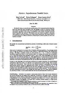
Parallelization of the n-fold Way Algorithm for Potts Model Lubachevsky (Lubachevsky 1987, 1988) proposed parallelization of the Ising model based on an asynchronous scheme. Korniss et al. (1999) developed a parallel MC model for studying magnetic domains using Lubachevsky approach. The main ideas involved in the asynchronous parallelization of the n-fold way algorithm for Ising-like systems are described as follows. The first step in parallelization involves dividing the simulation domain into suitably sized pieces for each processor to work with. One such example of domain decomposition is shown in Figure 1. Each processor works on its piece of simulation domain with its local simulation time. When a processor chooses a site that is situated on a processor boundary or a corner, special care must be taken to ensure that the simulation trajectory is not corrupted. This is achieved by allowing a border or corner site update only if its local simulation time is less than or equal to the local times of all the corresponding processors that carry its neighboring sites. For example, in Figure 1, if the processor 0 has chosen the diamond-patterned site to update, then this update will be evaluated only when the local simulation time

of processor 0 becomes less than or equal to the local simulation time of processors 1, 3 and 4 that carry the neighboring sites marked with circles. PE0

PE1

PE2

PE3

PE5

PE6

PE7

PE8

Figure 1: Domain decomposition in parallel processing. In the example shown in the figure, a global simulation domain size of 12 x 12 sites is divided up into 9 processors, each carrying a local simulation domain size of 4 x 4 sites. Note that the sites situated at a processor corner (e.g. marked with a diamond pattern above) have some of their neighbors located on three other processors (filled with gray color), sites at a processor boundary (vertical line pattern) have some of their neighbors residing in one other processor (horizontal line pattern) while sites within the kernel of the local domain (marked with dotted pattern) have all of its neighbors within the same processor. The numbers shown are the processing element (PE) or processor ID numbers. Until this happen, processor 0 must wait. Lubachevsky and Korniss et al. defined a special class for boundary and corner sites to handle PE boundaries. The activity of all of the PE boundary and corner sites was always set to 1. Assigning a high weight to PE boundary sites leads to PE boundary sites being picked more often and this compensate for the waiting at the PE boundaries This procedure ensures comparable evolution kinetics of the kernel and boundary sites. The time increment in the parallel n-fold way is given as: #t =

"1 n

ln r

(8)

Nb + ! n j p j j =1

Where Nb is the total number of sites on PE boundaries. The parallel n-fold way algorithm based on the asynchronous approach is then stated as follows: 1. Select a class based on Eq. 4. Note that in parallel, asynchronous n-fold way, PE boundary sites have a class of their own as explained above. 2. (a) If the chosen site is in kernel, flip it with probability 1 and go to Step 3 (b) If the chosen site is in the boundary class, then wait until the local simulation time of this updates becomes less than or equal to the local simulation times of the neighboring

PEs. When this condition is satisfied, evaluate the environment, compute transition probability and flip with Metropolis probability, Eq. 2. Go to Step 3. 3. Update tabulation of spin classes in kernel 4. Determine time of next update based on Eq. 8 5. Go to 1 until sufficient data is gathered. Problem of Kinetics in Lubachevsky Asynchronous Algorithm The grain growth kinetics results obtained using the above algorithm are shown in Figure 2 along with the results from scalar n-fold way for comparison. 180 x 180, 4 PEs, PSC, A = -1.79, B = 0.979 360 x 360 Chicoma, Scalar, A = -1.92 , B = 0.956 Log10(Average Grain Area)

1000

log(Area) = A - BLog(Time)

100

10

1000

10000

100000

Log10(Time)

Figure 2: Comparison of grain growth kinetics obtained in scalar and parallel version. It can be seen from Fig. 2 that while the grain growth exponent obtained in scalar and parallel version is close to 1.0 as expected, but the two lines do not overlap and the difference between the kinetics is diverging as time progresses. Also, the Log A vs. Log t curve for the parallel version appears to be curving and diverging away from the scalar result. This behaviour was analyzed and I believe that the discrepancy between the parallel and scalar kinetics is caused by the accounting of time in the versions as explained below. Time increment of n-fold way scalar version is given as follows:

#t s =

"1 n

! ni p i

x ln r1

1

The time increment of n-fold way parallel version is given by the following equation:

(9)

"1

#t p =

n

N b + ! ni p i

(10)

x ln r2

1

Taking the ratio of Eqs. (9) and (10), ignoring the ratio of natural logarithm of random numbers and rearranging leads to: n

" ni p i 1

!t p =

n

N b + " ni p i

(11)

x!t s

1

It is now evident that the denominator in the first term of Eq. (11) is always greater than its numerator (except for the trivial case when t = 0 when the ratio may be 1), and therefore the time increment in the parallel algorithm is always smaller than its scalar counterpart. This is because the activity of PE boundary sites is always set to 1 regardless of the configuration of its neighbors to give them a greater chance of being picked as explained before. This behaviour is reflected in Fig. 2, which clearly shows the faster evolution kinetics in parallel version (for any given grain area, parallel version indicates a smaller simulation time compared to scalar version). Korniss et al. (1999) have also suggested that parallel time increment is smaller that the scalar time increment. At long times, a large number of PE boundary sites happen to be internal to some grain and as such in scalar algorithm their activity is 0 while in parallel algorithm their activity is 1. This leads to increasing divergence in the computation of the simulation time in the two versions as seen in Fig. 2. The variation of the number of sites at PE boundary those are internal to a grain as a function of evolution is shown in Figure 3.

Global PE Bdy Sites That Are Internal to Some Grain (%)

100

180 x 180, 4 PEs, PSC, 5/8/03

90 80 70 60 The graph shows that as the structure evolves, the percentage of PE boundary sites that are internal to some grain increases. This leads to underestimation of program time in parallel algorithm compared to its scalar couterpart. Setting of PE bdy sites activity always to 1 causes these sites to be picked more often, but it also leads to a smaller time step. It is possible to compesate for this effect in the program.

50 40 30 20 10 0 0

500

1000

1500

2000

2500

NFW_Iterations (x1000)

Figure 3: Variation of PE boundary sites that are internal to a grain as a function of evolution. It is clear from Figure 3 that a larger proportion of sites at the PE boundaries also happen to be internal to some grain and as such their activity should have been 0 while it is treated as 1 in Lubachevsky algorithm leading to the calculation of relatively smaller time increment according to Eq. 10. This

problem is solved to a large extent by using a variation of Lubachevsky algorithm as proposed in the following section. Algorithm Proposed in this Work The proposed algorithm is stated as follows: i

N "1

i +1

0

0

0

1. Select a site and spin number to flip to based on ! p i < (drand48 ()* ! pi )< ! p i 2. (a) If the chosen site is in kernel of a PE, flip it with a probability 1 and go to Step 3. (b) If the chosen site is on the boundary of a PE, then wait until the local simulation time of this updates becomes less than or equal to the local simulation time of the relevant neighboring PEs. Whenever this condition is satisfied, then the site may or may not be able to flip. Go to Step 3. 3. Adjust PE boundary conditions. Note: PE boundary sites are not permitted to look at these neighboring boundaries until they pass the condition in Step 2b because the neighboring boundary sites have different time stamps as they come from different PEs. 4. Update transition probability for this site (after successful flip) and its neighboring sites. If this site or any of its neighbors lie on a PE boundary, then update their probability with the following rule: set the probability to 1 when the number of like neighbors within its PE are < 5 else set it 0. 5. Update simulation time whenever the site flipped successfully or whenever site did not flip due to rejection in Step 2b. Do not update time when the chosen site was on PE boundary and also happened to be a site internal to some grain that has grown across the PE boundaries. This is discussed in the following section in more detail. 6. Go to Step 1 until done.

5. Special Issues due to Asynchronous Parallelization 5.1 Getting Equilibrium Physics Right at PE Boundaries Dr. James Morris raised this problem during my talk at CMSN meeting in Iowa. He suggested that sites at PE boundaries might be at disadvantage due to the wait directive in Step 2b compared to the sites

within the kernel of a PEs. As a result, it was likely that grain boundaries may move more slowly across the PE boundaries compared to their movement within a PE. Dr. Morris thus suggested that the rate of grain growth at PE boundary would not be identical to that of grains within PE kernel as it should be when the laws of equilibrium physics are followed correctly during the simulation. This problem was analyzed later and it was found that ratio of GB Sites Internal to a PE divided by GB Sites on PE boundary did not remain constant throughout microstructure evolution. This confirmed Dr. Morris’s suggestion. I visited him in Iowa and discussed this matter in more detail. Based on these discussions and the approach suggested by Korniss et al. it was suggested that the PE boundary sites be picked more frequently compared to the kernel sites so that the disadvantage of the wait directive is exactly nullified. This was done by setting the “activity” (normalized transition probability) of all PE boundary sites to 1 regardless of their surrounding configuration. The result of this modification is shown in Figure 1. It is clear from Fig. 1 that ratio of GB sites internal to PE to that at PE boundaries is closer to an initial value of ~ 24.25 throughout the evolution. 5.2 Getting the Process Kinetics Right

6. Resolution of Special Issues The problem is solved by correcting for the error identified in Section 5.2. This is done by computing the environment of the PE boundary sites that is contained within a PE. What this means is that for each PE boundary site there are 5 neighbors in its time frame because sites in a domain within a PE share the same local simulation time while 3 neighbors that come from an adjacent PE have a different local time. The criteria for a site to be considered internal to a grain is that all five neighbors in the PE domain are in the same state (i.e. have the same spin number) as the site being evaluated, then such a site is an grain interior site. The activity of this site is set 0 and not to 1 as suggested in Korniss et al. and Lubachevsky version. PE corner site activity is always set 1 regardless of the neighbor’s state. The suggested criteria does not violate n-fold way algorithm because the unevaluated neighbors may have any state, however the site is not going to flip any of those neighbors because the Metropolis et al. transition probability for such a flip is 0 as ΔE > 0 for such a transition. By incorporating this modification in the asynchronous algorithm, the discrepancy between the scalar and parallel time steps is decreased significantly as shown in the following section. 7. Results: Good News At Last! 7.1 Getting Equilibrium Physics Right at PE Boundaries The variation of the ratio of the GB sites internal to a PE to that at PE boundaries as a function of evolution is shown in Figure 4. It is clear from Fig. 4 that suggested modification does not adversely affect the evolution of the ratio and it better than the old version and sometimes even better than the original asynchronous version.

old data modasync.c async.c

GB Sites Internal to PE -------------------------------GB Sites on PE Bdy 30

Initial ~ 24.25

25 20 15 10 5 0 10

20

40

60

80

100

200

400

600

800

Iterations (x1000)

Figure 4: Comparison of ratio of GB sites internal to grain to GB sites on PE boundary as a function of evolution. In the asynchronous algorithm (ames.c), PE site activity is always set 1, in the modified asynchronous algorithm (current work – modames.c) the activity is set to 0 if all of the neighbors within the PE are same else it is set to 1. Old data is based on the computing the activity based on all neighbors. Another way of looking at this is shown in Figure 5 below.

PEBdyGBSites/MaxPEBdySites PEInternalGBSites/MaxPEInternalSites 100

Ratio (%)

80

60

40

20

0 10

20

30

40

50 100 200 300 400 500 600 800 1000

Iterations (x1000)

Figure 5: Variation of PE boundary and internal grain boundary sites as a function of evolution. It is evident from Fig. 5 that GB sites both internal to and at boundary of a PE decrease as evolution progresses. However, the critical observation is that this decrease is comparable in both cases as shown in Fig. 5.

7.2 Getting the Process Kinetics Right The kinetics of grain growth obtained in scalar and parallel version developed in this work is shown in Figure 6. 200 x 200, chicoma, chiames.c 100 x 100, 4 PEs, modasync.c

Log10(Average Grian Area)

1000

100

10

1 100

1000

10000

100000

Log10(Program Time)

Figure 6: Comparison of grain growth obtained in scalar and parallel versions. It is clear that there is no discernible difference in the grain growth kinetics obtained in scalar and parallel version except at the very late stage where only a few grains (~10 – 20 grains) are left in the system. The grain growth exponent obtained in scalar and parallel versions is close to 1 and the pre-factors are also similar as shown in Figure 7. Grain size distribution obtained in parallel version is shown in Figure 8, which indicates a reasonable lognormal fit. 610 Grains, 100,000 Iterations 0.10

Data: MODASYNC2_B Model: LogNormal2 Chi^2 = 0.00006 R^2 = 0.96299

0.06

y0 A xc w

Normalized Frequency

0.08

-0.00386 ±0.00369 0.10467 ±0.00431 0.7624 ±0.01595 0.49729 ±0.0311

0.04

0.02

0.00 0.0

0.5

1.0

1.5

2.0

Normalized Grain Diameter

2.5

3.0

Figure 8: Grain size distribution obtained in parallel version. 8. Conclusions • • •

An asynchronous parallel algorithm is implemented for Potts model and applied for grain growth simulation in single-phase isotropic systems. Asynchronous algorithm is modified to remove the errors caused by setting the PE boundary site activity always to 1 in the original version (Lubachevsky) and its implementation (Korniss et al.) of the algorithm. Results obtained based on the modified asynchronous algorithm demonstrate:  Equivalent evolution rate of the sites at PE boundary and internal (Fig. 5)  Close agreement between scalar and parallel process kinetics  Linear grain growth kinetics with an exponent close to 1  Grain size distribution described by a log-normal function form

References Anderson, M., G. Grest, et al. (1989). "Computer simulation of normal grain growth in three dimensions." Phil. Mag. B 59(3): 293-329. Bortz, A. B., Kalos, M. H., Lebowitz, J. L. (1975). "A new algorithm for Monte Carlo simulations of Ising spin systems." Journal of Computational Physics 17: 10-18. Hassold, G. N. and E. A. Holm (1993). "A fast serial algorithm for the finite temperature quenched Potts model." Computers in Physics 7(1): 97-107. Ising, E. (1925). "Beitrag zue Theorie des Ferromagnetismus." (Contribution to the theory of ferromagnetism) Zeitschrift für Physik, 31: 253-258. K-Y. Jung, P. Manohar and A. D. Rollett (2002). “New Methods for Computer Simulation of Microstructural Evolution in 3D”, TMS Fall Meeting and ‘Materials Solutions’ conference, Columbus, Ohio, USA, October 6 – 10. Landau, D. P. and K. Binder (2000). A Guide to Monte Carlo Simulations in Statistical Physics. Cambridge, England, Cambridge University Press. Lubachevsky, B. D. (1988). “Efficient parallel simulations of dynamic Ising spin systems.” Journal of Computational Physics, 75: 103 – 122. Lubachevsky, B. D. (1987). “Efficient parallel simulations of dynamic Ising spin systems.” Complex Systems, 1: 1099 – 1123. Metropolis, N., Rosenbluth, A. W., Rosenbluth, M. N., Teller, A. H., and Teller, E. (1953). "Equation of state calculations by fast computing machines." J. Chemical Physics 21(6): 1087-1092. Miodownik, M., A. Godfrey, et al. (1999). "On boundary misorientation distribution functions and how to incorporate them into three-dimensional models of microstructural evolution." Acta materiala 47(9): 2661-2668. Miodownik, M., E. Holm, et al. (2000). "Highly parallel computer simulations of particle pinning: Zener vindicated." Scripta Materiala 42: 1173-1177. Novotny M. A. (1995). “A new approach to an old algorithm for the simulation of Ising-like systems”, Computers in Physics, 9(1): 46 – 52. R. B. Potts R. B. (1952). “Some generalized order-disorder transitions”, Proc. Cambridge Philosophical Society, 48: 106 – 109. A. D. Rollett (2002). “Towards Realistic Mesoscopic Methods for Microstructural Evolution”, TMS Fall Meeting and ‘Materials Solutions’ conference, Columbus, Ohio, USA, October 6 – 10.

Rollett, A. D., M. J. Luton, et al. (1992). "Computer Simulation of Dynamic Recrystallization." Acta metall. mater. 40: 43-55. Rollett, A. D. and W. W. Mullins (1996). "On the growth of abnormal grains." Scripta metall. et mater. 36(9): 975-980. Rollett, A. D. and D. Raabe (2001). "A Hybrid Model for Mesoscopic Simulation of Recrystallization." Computational Materials Science 21(1): 69-78. Rollett, A. D., D. J. Srolovitz, et al. (1989). "Simulation and Theory of Abnormal Grain GrowthVariable Grain Boundary Energies and Mobilities." Acta Metall. 37: 2127. Rollett, A. D., D. J. Srolovitz, et al. (1992). "Computer Simulation of Recrystallization - III. Influence of a Dispersion of Fine Particles." Acta Metallurgica 40: 3475-3495. Rollett, A. D., D. J. Srolovitz, et al. (1989). "Computer Simulation of Recrystallization in NonUniformly Deformed Metals." Acta Metall. 37: 627. Sahni, P., D. Srolovitz, et al. (1983). "Kinetics of ordering in two dimensions. II. Quenched systems." Phys. Rev. B 28: 2705. Srolovitz, D. J., M. P. Anderson, et al. (1984). "Computer simulation of grain growth- III. influence of a particle dispersion." Acta metallurgica 32: 1429-1438. Srolovitz, D. J., M. P. Anderson, et al. (1984). "Computer simulation of grain growth - II. grain size distribution, topology and local dynamics." Acta metallurgica 32: 793. Srolovitz, D. J., G. S. Grest, et al. (1986). "Computer simulation of recrystallization- I. Homogeneous nucleation and growth." Acta metallurgica 34: 1833-1845. Srolovitz, D. J., G. S. Grest, et al. (1988). "Computer simulation of recrystallization: II. Heterogenous Nucleation and Growth." Acta metallurgica 36(8): 2115-2128. Upmanyu, M., D. Srolovitz, et al. (1998). "Atomistic simulation of curvature driven grain boundary migration." Interface Science 6(1-2): 41-58.