Aug 8, 2016 - In CRST, the requirement on the invariant mass of the two highest-weight b-tagged jets, mbb, is used to reject t¯tcontamination from the control ...
ATLAS NOTE ATLAS-CONF-2016-077 4th August 2016
Search for a Scalar Partner of the Top Quark in the Jets+E miss T √ Final State at s = 13 TeV with the ATLAS detector The ATLAS Collaboration
08 August 2016
ATLAS-CONF-2016-077
Abstract A search for direct pair production of a scalar partner to the top quark in events with four −1 or √ more jets plus missing transverse momentum is presented. An analysis of 13.3 fb of s = 13 TeV proton-proton collisions collected using the ATLAS detector at the LHC yielded no significant excess over the Standard Model background expectation. In the supersymmetric 0 ± 0 interpretation, the top squark is assumed to decay via t˜ → t χ˜ 1 , t˜ → b χ˜ 1 → bW (∗) χ˜ 1 , or 0 0 ± t˜ → bW χ˜ 1 , where χ˜ 1 ( χ˜ 1 ) denotes the lightest neutralino (chargino). Exclusion limits are reported in terms of the top squark and neutralino masses. Assuming branching fractions of 0 0 100% to t χ˜ 1 , top squark masses in the range 310–820 GeV are excluded for χ˜ 1 masses below 160 GeV. In the case where mt˜ ∼ mt + m χ˜ 0 top squark masses between 23–380 GeV are excluded. Limits are also reported in terms of simplified models describing the associated production of dark matter ( χ) with top quark pairs through a (pseudo)scalar mediator; models with a global coupling of 3.5, mediator masses up to 300 GeV, and χ masses below 40 GeV are excluded.
© 2016 CERN for the benefit of the ATLAS Collaboration. Reproduction of this article or parts of it is allowed as specified in the CC-BY-4.0 license.
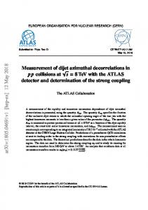
1. Introduction Supersymmetry (SUSY) is an extension of the Standard Model (SM) that can resolve the gauge hierarchy problem [1–6] by introducing supersymmetric partners of the known bosons and fermions. The SUSY partner to the top quark, the top squark1 (t˜), plays an important role in canceling the dominant top quark loop diagram contributions to the divergence of the Higgs boson mass. In R-parity conserving SUSY models [7–10], the supersymmetric partners are produced in pairs. The cross section for direct pair production of top squarks is given by gluon-gluon and q q¯ fusion and is largely decoupled from SUSY model parameters [11–13]. The decay of the top squark depends on the masses, the mixing of the left- and right-handed t˜ quarks and the mixing parameters of the fermionic partners of the electroweak and Higgs bosons which are collectively known as charginos, χ˜ ±i , i = 1, 2 and neutralinos, 0 ± 0 χ˜ 0i , i = 1–4. Three different decay modes are considered: (a) t˜ → t χ˜ 1 , (b) t˜ → b χ˜ 1 → bW (∗) χ˜ 1 , or (c) 0 0 t˜ → bW χ˜ 1 , as illustrated in Fig. 1(a)−(c), respectively. The lightest neutralino, χ˜ 1 , is assumed to be the stable, weakly interacting lightest supersymmetric particle2 that also serves as a dark matter candidate [14, 15]. In addition to direct pair production, top squarks can be produced indirectly through gluino decays, as shown in Fig. 1(d). This search considers models where the mass difference between the top squark and 0 the neutralino is small, i.e., ∆m(t˜, χ˜ 1 ) = 5 GeV. In this scenario, the jets originating from the t˜ decays have small momenta compared to experimental acceptance resulting in a nearly identical signature to 0 t˜ → t χ˜ 1 signal models. Finally, a simplified model of top quark pairs produced in association with a pair of dark matter (DM) particles is also considered [16, 17]. As illustrated in Fig. 1(e), a pair of DM particles (each represented by χ) are produced via a spin-0 mediator (ϕ or a). This mediator can be a scalar or pseudoscalar and is coupled to the SM particles by mixing with the SM Higgs or extended Higgs sector. R This note presents the search for direct top squark pair production using L dt = (13.3 ± 0.4) fb−1 of √ pp collisions provided by the Large Hadron Collider (LHC) at a center-of-mass energy of s = 13 TeV. These data were collected by the ATLAS detector in 2015 and 2016. All-hadronic final states with at miss least four jets and large missing transverse momentum (pmiss T , whose magnitude is referred to as ET ) are considered, and the results are interpreted according to a variety of signal models as described above. Signal regions are defined to maximize the experimental sensitivity over a large range of kinematic phase space with various specializations. Sensitivity to high top squark masses ∼ 850 GeV (as in Fig. 1(a)) and top squarks produced through gluino decays (as in Fig. 1(d)) are achieved by exploiting techniques designed to reconstruct Lorentz-boosted top quarks. The dominant SM background process for this ± kinematic region is Z → ν ν¯ plus heavy flavor jets. The sensitivity to the decay b χ˜ 1 is enhanced by vetoing events containing hadronically decaying top quark candidates. Sensitivity to the region where mt˜ − m χ˜ 0 ∼ mt , which nominally has low-pT final state objects and low ETmiss , is achieved by exploiting 1 events in which initial state radiation (ISR) boosts the di-top-squark system in the transverse plane. For this regime, t t¯ production makes up the dominant background contribution. Similar searches based on √ √ s = 7 TeV and s = 8 TeV data collected at Run 1 of the LHC have been performed by both the ATLAS [18, 19] and CMS [20–25] collaborations. 1
The superpartners of the left- and right- handed top quarks, t˜L and t˜R , mix to form the two mass eigenstates t˜1 and t˜2 , where t˜1 is the lighter one. Throughout this note t˜1 is noted as t˜. 2 However, the lightest supersymmetric particle could also be a very light gravitino (the fermionic partner of the graviton), which would evade existing model-dependent limits on the neutralino mass.
2
(a) t˜ → t χ˜ 1
0 ± (b) t˜ → b χ˜ 1 → bW (∗) χ˜ 1
0
(c) t˜ → bW χ˜ 1 0
g
t
t
sof t
p g˜ g˜
p
¯
χ ˜01
t˜ t˜
'/a
χ ˜01 sof t
g
t
(d) g˜ → t t˜ → t χ˜ 1 +soft 0
t
(e) DM+t t¯
Figure 1: The decay topologies of the signal models considered with experimental signatures of four or more jets plus missing transverse momentum.
The following sections detail the ATLAS detector, trigger and data collection, as well as the simulated event samples used in the analysis. This is followed by a description of the event and physics object reconstruction and the signal region definitions. The procedures and control regions used to estimate the backgrounds in each of the signal regions are described, as well as the evaluation of systematic uncertainties, followed by the presentation of the results and their interpretation. 1
2. ATLAS detector The ATLAS experiment [26] at the LHC is a multi-purpose particle detector with a forward-backward symmetric geometry3 and a near 4π coverage in solid angle. It consists of an inner tracking detector surrounded by a thin superconducting solenoid providing a 2 T axial magnetic field, electromagnetic and hadron calorimeters, and a muon spectrometer. The inner tracking detector covers the pseudorapidity range |η| < 2.5. It consists of silicon pixel, silicon micro-strip, and transition radiation tracking detectors. The newly installed innermost layer of pixel sensors [27] was operational for the first time during the 2015 data taking. Lead/liquid-argon (LAr) sampling calorimeters provide electromagnetic (EM) energy measurements with high granularity. A hadron (steel/scintillator-tile) calorimeter covers the central pseudorapidity range (|η| < 1.7). The end-cap and forward regions are instrumented with LAr calorimeters 3
ATLAS uses a right-handed coordinate system with its origin at the nominal interaction point (IP) in the centre of the detector and the z-axis along the beam pipe. The x-axis points from the IP to the centre of the LHC ring, and the y-axis points upwards. Cylindrical coordinates (r, φ) are used in the transverse plane, φ being the azimuthal angle around the z-axis. The pseudorapidity is defined in terms of the polar angle θ as η = − ln tan(θ/2). Angular distance is measured in units of q ∆R ≡
(∆η) 2 + (∆φ) 2 .
3
for both EM and hadronic energy measurements up to |η| = 4.9. The muon spectrometer surrounds the calorimeters and is based on three large air-core toroid superconducting magnets with eight coils each. The toroid field strength is 0.5 T in the central region and 1 T in the end-cap regions. It includes a system of precision tracking chambers and fast detectors for triggering.
3. Trigger and data collection The data were collected from August to November 2015 and April to July 2016 at a pp centre-of-mass energy of 13 TeV with 25 ns bunch spacing. A two-level trigger system is used to select events. The first-level trigger is implemented in hardware and uses a subset of the detector information to reduce the accepted rate to at most 100 kHz. This is followed by a software-based trigger that reduces the accepted event rate to 1 kHz for offline storage. For the primary search region, a missing transverse momentum trigger was used for 2015 data which bases the bulk of its rejection on the vector sum of transverse energies deposited in projective trigger towers (each with a size of approximately ∆η × ∆φ ∼ 0.1 × 0.1 for |η| < 2.5; these are larger and less regular in the more forward regions). A more refined calculation, based on the vector sum of all calorimeter cells, is used at a later stage in the trigger processing, requiring an energy threshold of 70 GeV. Due to the increase in instantaneous luminosity in 2016 data a higher threshold of 100 GeV is used with a different trigger algorithm which is based on the transverse vector sum of all reconstructed jets. Data events were collected using these triggers, which are fully efficient for offline calibrated ETmiss > 250 GeV in signal events. The luminosity uncertainty of 2.1% (3.7%) for data taken in 2015 (2016) is derived following the same methodology as that detailed in Refs. [28] and [29], from a preliminary calibration of the luminosity scale obtained from beam-separation scans performed in August 2015 (May 2016). Data samples enriched in the major sources of background were collected with electron or muon triggers. The electron trigger selects events based on the presence of clusters of energy in the electromagnetic calorimeter, with a shower shape consistent with that of an electron, and a matching track in the tracking system. The muon trigger selects events containing one or more muon candidates based on tracks identified in the muon spectrometer and inner detector. The transverse momentum threshold required by triggers in 2015 is 24 GeV for electrons and 20 GeV for muons. Due to the higher instantaneous luminosity in 2016 the trigger threshold was increased to 26 GeV for both electrons and muons and a tight isolation requirement is applied. In order to recover some of the efficiency for high-pT leptons, events were also collected with single-electron and single-muon triggers with looser or no isolation requirements, but with higher pT thresholds (pT > 60 GeV and pT > 50 GeV, respectively). Finally, a single-electron trigger requiring pT > 120 GeV (in 2015) and pT > 140 GeV (in 2016) with less restrictive electron identification criteria is used to increase the selection efficiency for high-pT electrons. The electron and muon triggers used are > 99% efficient for electrons and muons with pT of 2 GeV greater than the trigger thresholds. Triggers based on the presence of high-pT jets are used to collect data samples for the estimation of the multijet and all-hadronic t t¯ background. The jet pT thresholds ranged from 20 to 400 GeV. In order to stay within the bandwidth limits of the trigger system, only a fraction of events passing these triggers were recorded to permanent storage.
4
4. Simulated samples and signal modelling Simulated events are used to model the SUSY signal and to aid in the description of the background processes. Several configurations are used for the signal samples, as shown in Fig. 1: (a) both top squarks 0 0 decay via t˜ → t χ˜ 1 , with ∆m(t˜, χ˜ 1 ) > mt , where mt is the mass of the top quark, (b) both top squarks 0 ± 0 ± decay via t˜ → b χ˜ 1 → bW (∗) χ˜ 1 , where m( χ˜ 1 ) = 2m( χ˜ 1 ) which is motivated by gaugino universality, 0 0 and (c) three body decays via t˜ → bW χ˜ 1 , where m(b) + m(W ) < ∆m(t˜, χ˜ 1 ) < mt . These signal samples 0 are generated in a grid across the plane of the top squark and χ˜ 1 masses with a grid spacing of 50 GeV across most of the plane. Gluino-mediated t˜ production is also simulated (as shown in Fig. 1(d)), in which 0 gluinos decay via g˜ → t t˜, with the t˜ always decaying to low momenta objects and χ˜ 1 . The mass difference 0 ∆m(t˜, χ˜ 1 ) is set to 5 GeV, and a range of gluino and top squark masses are generated. Finally (as shown in Fig. 1(e)), the associated production of a t t¯ pair and a pair of dark matter particles is simulated for a range of mediator and dark matter particle masses. In order to fulfill precision constraints from flavor measurements, the model assumes Yukawa-like couplings between the dark sector mediator and the SM fermions. This motivates the choice of studying these models in heavy flavor quark final states. The model has five free parameters [30, 31] corresponding to the mass of the mediator and the DM particle, the coupling of the mediator with the DM and SM particles, and the width of the mediator. The mediator width is assumed to be the minimal width that can be calculated from all parameters of the model. The signal grid is generated by scanning over the mass parameters. The coupling of the mediator to the dark matter particle (g χ ) is set to be equal to its coupling to the quarks (gq ) and cross sections corresponding to a range of couplings are considered. The minimum mediator coupling considered is 0.1 and the maximum mediator coupling considered is 3.5, at the perturbative limit, and has the same strength for SM and DM particles. The aforementioned signal models are all generated with MadGraph5_aMC@NLO [32] interfaced to PYTHIA 8 [33] for the parton showering (PS) and hadronisation and with EvtGen v1.2.0 program [34] as afterburner. The matrix element (ME) calculation is performed at tree-level and includes the emission of up to two additional partons for the t˜ samples but not for the DM ones. The parton distribution function (PDF) set used for the generation of the t˜ samples is NNPDF2.3LO [35] (NNPDF3.0NLO for the DM) and the A14 set [36] of underlying-event tuned parameters (UE tune). For the direct t˜ pair production samples, the ME-PS matching is performed with the CKKW-L [37] prescription, with a matching scale set to one quarter of the mass of the t˜. Signal cross sections are calculated to next-to-leading order in the strong coupling constant, adding the resummation of soft gluon emission at next-to-leading-logarithmic accuracy (NLO+NLL) [11–13]. The nominal cross section and the uncertainty are taken from an envelope of cross section predictions using different PDF sets and factorization and renormalization scales, as described in Ref. [38]. SM background samples are generated with different MC generators depending on the process. The background sources of Z + jets and W + jets are generated with SHERPAv2.2.0 [39] using NNPDF3.0NNLO [35] PDF set and the default tune. Top quark pair production where at least one of the top quarks decays to a lepton and single top production are simulated with Powheg-Boxv.2 [40] and interfaced to PYTHIA6 [41] for PS and hadronisation, with CT10 [42] PDF set and using the P2012 [43] set of tuned parameters. MadGraph5_aMC@NLO interfaced to PYTHIA 8 for PS and hadronisation is used to generate the t t¯+V samples at NLO with the NNPDF3.0NLO PDF set. The underlying tune used is A14 with the NNPDF2.3LO PDF set. Finally, dibosons are generated with SHERPAv2.1.1 using CT10 PDF set. Additional information can be found in Refs. [44–48].
5
The detector simulation [49] is performed using either GEANT4 [50] or a fast simulation framework where the showers in the electromagnetic and hadronic calorimeters are simulated with a parameterized description [51] and the rest of the detector is simulated with GEANT4. The fast simulation was validated against full GEANT4 simulation for several selected signal samples. All MC samples are produced with a varying number of simulated minimum-bias interactions overlaid on the hard-scattering event to account for multiple pp interactions in the same or nearby bunch crossing (pileup). The simulated events are reweighted to match the distribution in data. Corrections are applied to the simulated events to correct for differences between data and simulation for the lepton trigger and reconstruction efficiencies, momentum scale, energy resolution, isolation, and for the efficiency of identifying jets originating from the fragmentation of b-quarks, together with the probability for mis-tagging light-flavor and charm quarks.
5. Event and physics object reconstruction Events are required to have a primary vertex [52] reconstructed from at least two associated tracks with pT > 400 MeV and which are compatible with originating from the luminous region. If more than one such vertex is found, the vertex with the largest summed pT2 of the associated tracks is chosen. Jets are reconstructed from three-dimensional topological clusters of noise-suppressed calorimeter cells [53] using the anti-k t jet algorithm [54] with a distance parameter R = 0.4. An area-based correction is applied to account for energy from additional pp collisions based on an estimate of the pileup activity in a given event [55]. Calibrated [56] jets are required to have pT > 20 GeV and |η| < 2.8. Events containing jets arising from non-collision sources or detector noise [57] are removed from consideration. Additional selections are applied to jets with pT < 60 GeV and |η| < 2.4 to reject events that originate from pileup interactions [58]. Jets initiated by a b-quark and which are within the inner detector acceptance (|η| < 2.5) are identified with a multivariate algorithm that exploits the impact parameters of the charged-particle tracks, the presence of secondary vertices and the reconstructed flight paths of b- and c-hadrons inside the jet [59–61]. The average identification efficiency of jets containing b-quarks is 77% as measured with simulated t t¯ events. A rejection factor of approximately 134 is reached for light-quark and gluon jets (depending on the pT of the jet) and 6.2 for charm jets. Electron candidates are reconstructed from energy clusters in the electromagnetic calorimeter that are matched to a track in the inner detector. They are required to have |η| < 2.47, pT > 7 GeV and must pass a variant of the “very loose” likelihood-based selection. In the case where the separation between an electron candidate and a non-b-tagged (b-tagged) jet is ∆R < 0.24, the object is considered to be an electron (b-tagged jet). If the separation between an electron candidate and any jet satisfies 0.2 < ∆R < 0.4, the object is considered to be a jet. Muons are reconstructed from matching tracks in the inner detector and in the muon spectrometer and are required to have |η| < 2.7, pT > 6 GeV. If the separation between a muon and any jet is ∆R < 0.4, the muon is omitted. is the negative vector sum of the pT of all selected and calibrated physics objects in the event. The pmiss T An extra term is added to account for soft energy in the event that is not associated to any of the selected objects. This soft term is calculated from inner detector tracks with pT > 400 MeV matched to the primary vertex to make it more resilient to pileup contaminations [62]. The missing transverse momentum from the tracking system (denoted as pmiss,track , with magnitude ETmiss,track ) is computed from the vector sum of T 4
For the overlap removal, rapidity is used instead of pseudorapidity in the ∆R definition.
6
the reconstructed inner detector tracks with pT > 500 MeV, |η| < 2.5, that are associated with the primary vertex in the event. The requirements on electrons and muons are tightened for the selection of events in background control regions (described in section 7) containing leptons. Both electron and muon candidates are required to have pT > 20 GeV and satisfy pT -dependent track- and calorimeter-based isolation criteria. Electron and muon candidates matched to trigger electron (muon) candidates must have pT exceeding the corresponding trigger threshold by at least 2 GeV. Electron candidates are required to pass a “tight” likelihood-based selection. The impact parameter of the electron in the transverse plane with respect to the reconstructed event primary vertex (|d 0 |) is required to be less than five times the impact parameter uncertainty (σ d0 ). The impact parameter along the beam direction, |z0 × sin θ|, is required to be less than 0.5 mm. Further selection criteria on reconstructed muons are also imposed: muon candidates are required to pass a “medium" quality selection [63]. In addition, the requirements |d 0 | < 3σ d0 and |z0 × sin θ| < 0.5 mm are imposed for muon candidates.
6. Signal region definitions The main experimental signature for all signal topologies is the presence of multiple jets (two of which originate from b-quarks), no leptons, and significant missing transverse momentum. A common preselection is defined for all signal regions. At least four jets are required, at least one of which must be b-tagged. The leading four jets must satisfy pT > 80, 80, 40, 40 GeV. Events containing reconstructed electrons or muons are vetoed. The ETmiss trigger dictates the requirement ETmiss > 250 GeV and rejects the majority of background from multijet and all-hadronic t t¯ events. In order to reject events with mis-measured ETmiss originating from multijet and hadronic t t¯ decays, an angular separation between � � the azimuthal angle of the two highest pT jets and the ETmiss is required: ∆φ jet0,1, ETmiss > 0.4. Further reduction of such events is attained by requiring the ETmiss,track to be aligned in φ with respect to the ETmiss � � calculated from the calorimeter system: ETmiss,track > 30 GeV and ∆φ ETmiss, ETmiss,track < π/3 radians.
Beyond these common requirements, six sets of signal regions (SRA-F) are defined to target each topology and kinematic regime. SRA (SRB) is sensitive to production of high-mass t˜ pairs with large (small) 0 ∆m(t˜, χ˜ ). Both SRA and SRB employ top mass reconstruction techniques to reject background. SRC is ± targeted at t˜ → b χ˜ 1 decays, where no top quark candidates are reconstructed. SRD is designed for the 0 highly compressed region with ∆m(t˜, χ˜ ) ∼ mt . In this signal region, initial state radiation (ISR) is used to improve sensitivity to these decays. SRE is aimed at dark matter + t t¯ final states, and SRF is optimized for scenarios with highly boosted top quarks that can occur in gluino-mediated top squark production. Signal Region Sets A and B SRA and SRB are targeted at direct top squark pair production where the top squarks decay via t˜ → t χ˜ 1 0 and ∆m(t˜, χ˜ 1 ) > mt . SRA is optimized for mt˜ = 800 GeV, m χ˜ 0 = 1 GeV while SRB is optimized for mt˜ = 600 GeV, m χ˜ 0 = 300 GeV. Two b-tagged jets are required. 0
The decay products of the t t¯ system in the all-hadronic decay mode can often be reconstructed as six distinct R = 0.4 jets. The transverse shape of these jets is typically circular with a radius equal to this distance parameter, but when two of the jets are less than 2R apart in η − φ space, the one-to-one correspondence
7
1000
ATLAS Preliminary s=13 TeV, 13.3 fb-1 preselection + m bT ,min>50 GeV
Events / 50 GeV
Events / 20 GeV
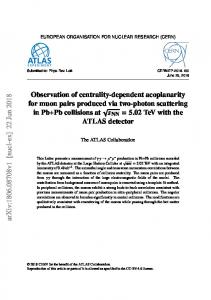
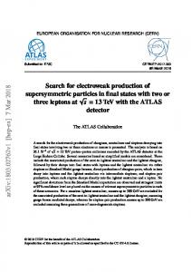
of a jet with a top daughter may no longer hold. Thus, the two hadronic top candidates are reconstructed by applying the anti-k t clustering algorithm [54] to the R = 0.4 jets, using reclustered distance parameters of R = 0.8 and R = 1.2. Two R = 1.2 reclustered jets are required; the mass of the highest pT R = 1.2 reclustered jet is shown in Fig. 2 (a). The events are divided into three categories based on the resulting R = 1.2 reclustered jet masses, as illustrated in Fig. 3: the “TT" category includes events with two well-reconstructed top candidates, the “TW” category contains events with one well-reconstructed top candidate and a well-reconstructed W candidate, and the “T0" category represents events with only one well-reconstructed top candidate. Since the signal-to-background ratio is quite different in each of these categories, they are optimized individually for both SRA and SRB.
Data SM Total tt Single Top tt+V
2000
ATLAS Preliminary s=13 TeV, 13.3 fb-1 preselection + m bT ,min>50 GeV
Data SM Total tt Single Top
1500
tt+V
W
W
Z
500
Data / SM
Data / SM
0 2.0
1.5 1.0 0.5 100
200
300
Diboson ~ 0 30.0 x (t1,∼ χ )=(600,300) GeV 1 ~ 0 30.0 x (t1,∼ χ )=(800,1) GeV
500
1
0.0 0
Z
1000
Diboson ~ 0 30.0 x (t1,∼ χ )=(600,300) GeV 1 ~ 0 30.0 x (t1,∼ χ )=(800,1) GeV
0 2.0
1.5 1.0 0.5 0.0 0
400
m 0jet, R =1.2 [GeV]
1
200
400
600
m bT,min [GeV]
(a)
(b)
Figure 2: Distributions of discriminating variables after the common preselection and an additional mTb,min > 50 GeV requirement. The stacked histograms show the SM expectation, normalized using scale factors derived from the simultaneous fit to all backgrounds. The “Data/SM" plots show the ratio of data events to the total SM expectation. The hatched uncertainty band around the SM expectation and in the ratio plots illustrates the combination of statistical and detector-related systematic uncertainties. The rightmost bin includes all overflows.
The most powerful discriminating variable against SM t t¯ production is the ETmiss resulting from the 0 undetected χ˜ 1 s. Substantial t t¯ background rejection is provided by additional requirements to reject events in which one W decays via a lepton plus neutrino. The first requirement is that the transverse mass (mT ) calculated from the ETmiss and the b-tagged jet closest in φ to the pmiss direction is above 200 GeV: T mTb,min =
q f � �g 2 pTb ETmiss 1 − cos ∆φ pTb, pmiss > 200 GeV, T
(1)
as illustrated in Fig. 2 (b). The second requirement is a “τ-veto” targeted at hadronic τ lepton candidates likely to have originated from a W → τν decay. Events that contain a non-b-tagged jet within |η| < 2.5 with ≤ 4 associated charged-particle tracks with pT > 500 MeV, and where the ∆φ between the jet and the pmiss is less than π/5 radians, are vetoed. In SRB, additional discrimination is provided by mTb,max and T ∆R(b, b). The former quantity is analogous to mTb,min except that the transverse mass is computed with direction. The latter quantity provides the b-tagged jet that has the largest ∆φ with respect to the pmiss T additional discrimination against background where the two b-tagged jets come from a gluon splitting. Table 1 summarizes the selection criteria that are used in these two signal regions.
8
ATLAS Preliminary Simulation s = 13 TeV ~ ∼0 ( t,χ ) = (800,1)
600
0.15
Expected Events
m 1jet, R =1.2 [GeV]
800
0.10
400
TT 200
0.05
TW T0
0 0
200
400
600
m 0jet, R =1.2
800
0.00
[GeV]
Figure 3: Illustration of signal region categories (TT, TW, and T0) based on the R = 1.2 reclustered top candidate 0 masses for simulated direct top squark pair production with (t˜, χ˜ 1 ) = (800, 1) GeV after the loose preselection requirement described in the text.
Signal Region Sets C ± SRC is optimized for direct top squark pair production where both top squarks decay via t˜ → b χ˜ 1 . In this signal region, at least four jets are required with pT > 150, 100, 40, 40 GeV, two of which must be b-tagged. SRC-low, SRC-med, and SRC-high are optimized for mt˜ = 400 GeV, m χ˜ 0 = 50 GeV, mt˜ = 600 GeV, m χ˜ 0 = 100 GeV, and mt˜ = 700 GeV, m χ˜ 0 = 50 GeV, respectively. The models considered ± 0 for the optimization have m( χ˜ 1 ) = 2m( χ˜ 1 ). Tighter leading and sub-leading jet pT requirements are made for SRC-med and SRC-high, as summarized in Table 2. Additional discrimination is provided by a √ miss miss measure of the ET significance: ET / HT , where HT is the scalar sum of the pT of all reconstructed √ √ √ R = 0.4 jets in an event. ETmiss / HT > 5 GeV is required, and an upper cut on this quantity of 12 GeV √ for the SRC-low and SRC-med regions and 17 GeV for the SRC-high region is applied.
The best sensitivity for this signal scenario is achieved by vetoing events with reconstructed top candidates. An alternative top reconstruction, with respect to the method used in the SRA and SRB selections, is used. The two jets with the highest weights from the b-tagging identification algorithm are selected. Among the remaining jets, the two closest in ∆R are combined to form a W candidate. The closest (in ∆R) high-weight b-tagged jet to this W candidate is then combined with it to form a top candidate. The mass of this resulting top candidate, mb j j , is then required to be > 250 GeV, ensuring background rejection in the low mb j j region. The high mb j j region, above the top mass, characteristically has less background contamination while still having significant signal contributions.
9
Table 1: Selection criteria for SRA and SRB, in addition to the common preselection requirements described in the text. The signal regions are separated into topological categories based on reconstructed top candidate masses.
Signal Region
TT
TW
T0
0 mjet, R=1.2
> 120 GeV
> 120 GeV
> 120 GeV
1 mjet, R=1.2
> 120 GeV
60 − 120 GeV
< 60 GeV
> 60 GeV
0 mjet, R=0.8
≥2
b-tagged jets SRA
mTb,min
> 200 GeV
τ-veto
yes > 400 GeV
ETmiss
> 450 GeV ≥2
b-tagged jets
SRB
> 500 GeV
mTb,min mTb,max
> 200 GeV
τ-veto
yes
> 200 GeV > 1.2
∆R (b, b)
> 250 GeV
ETmiss
Table 2: Selection criteria for SRC, in addition to the common preselection requirements described in the text.
Variable
SRC-low
SRC-med
mb j j
> 250 GeV
b-tagged jets
≥2
SRC-high
pT0
> 150 GeV
> 200 GeV
> 250 GeV
pT1
> 100 GeV
> 150 GeV
> 150 GeV
mTb,min
> 250 GeV
> 300 GeV
> 350 GeV
mTb,max
> 350 GeV
> 450 GeV
> 500 GeV
∆R(b, b) √ ETmiss / HT
√
> 0.8 √ [5, 12] GeV
√ [5, 17] GeV
[5, 12] GeV
> 250 GeV
ETmiss
10
Signal Region Sets D 0 SRD is optimized for direct top squark pair production where ∆m(t˜, χ˜ 1 ) ∼ mt , a regime in which the signal topology is extremely similar to SM t t¯ production. However, in the presence of high-momentum ISR, the di-top-squark system is boosted in the transverse plane. The ratio of the ETmiss to the pT of the ISR 0 system in the CM frame (pTISR ), defined as RISR , is proportional to the ratio of the χ˜ 1 and t˜ masses [64, 65]: E miss m χ˜10 RISR ≡ TISR ∼ . (2) mt˜ pT
A recursive jigsaw reconstruction technique, as described in Ref. [66], is used to divide each event into an ISR hemisphere and a sparticle hemisphere, where the latter consists of the pair of candidate top squarks, 0 each of which decays via a top quark and χ˜ 1 . Objects are grouped together based on their proximity in the lab frame’s transverse plane by minimizing the reconstructed transverse masses of the ISR system and sparticle system simultaneously over all choices of object assignment. Kinematic variables are then defined based on this assignment of objects to either the ISR system or the sparticle system. The selection criteria for this signal region are summarized in Table 3. The events are divided into eight windows defined by overlapping ranges of the reconstructed RISR , and target different top squark 0 and χ˜ 1 masses: e.g., SRD1 is optimized for mt˜ = 250 GeV, m χ˜ 0 = 77 GeV and SRD5 is optimized for mt˜ = 450 GeV, m χ˜ 0 = 277 GeV. Five jets or more are required to be assigned to the sparticle hemisphere of the event, and at least one (two) of those jets must be b-tagged in SRD1-4 (SRD5-8). Transverse b-tag,S momentum requirements on pTISR , the highest-pT b-jet in the sparticle hemisphere (pT ), and the jet 4,S fourth-highest-pT jet in the sparticle hemisphere (pT ) are applied. The transverse mass between the sparticle system and the ETmiss , defined as MTS , is required to be > 300 GeV. The ISR system is also required to be separated in azimuth from the ETmiss in the CM frame; this variable is defined as ∆φISR . Table 3: Selection criteria for SRD, in addition to the common preselection requirements described in the text. The signal regions are separated into windows based on ranges of RISR .
Variable
SRD1
SRD2
SRD3
SRD4
SRD5
SRD6
SRD7
SRD8
min RISR
0.25
0.30
0.35
0.40
0.45
0.50
0.55
0.60
max RISR
0.40
0.45
0.50
0.55
0.60
0.65
0.70
0.75
b-tagged jets
≥2
≥1
S Njet
≥5
pTISR b-tag,S pT jet 4,S pT MTS
> 400 GeV
∆φISR
> 3.0 radians
> 40 GeV > 50 GeV > 300 GeV
11
Signal Region E SRE is targeted at signal models of the associated production of top pairs with a pair of dark matter particles produced through a scalar (pseudoscalar) mediator ϕ (a) as illustrated in Fig. 1(e). Four or more reconstructed jets are required, two of which must be b-tagged. The discriminating variables considered have been described previously for SRA, SRB and SRC, but a dedicated optimization is performed using the mϕ = 350 GeV, m χ = 1 GeV simplified model as a benchmark. The resulting selection criteria are summarized in Table 4. Signal Region F SRF is designed for models which have highly boosted top quarks. Such signatures can arise from direct pair production of high-mass top partners, or from the gluino-mediated compressed t˜ scenario with large ∆m(g, ˜ t˜) as illustrated in Fig. 1(d). Four or more reconstructed jets are required, two of which must be b-tagged. In this regime, reclustered jets with R = 0.8 are utilized to optimize experimental sensitivity to these highly boosted top quarks. The selection criteria for SRF, optimized for mg˜ = 1400 GeV, mt˜ = 400 GeV, m χ˜ 0 = 395 GeV, are summarized in Table 4. Table 4: Selection criteria for SRE and SRF, in addition to the common preselection requirements described in the text.
Variable
SRE
SRF ≥2
b-tagged jets 0 mjet, R=1.2
> 140 GeV
-
1 mjet, R=1.2 0 mjet, R=0.8 1 mjet, R=0.8 b,min mT
> 60 GeV
-
-
> 120 GeV
-
> 60 GeV
> 200 GeV
> 175 GeV
τ−veto
yes
no
∆R(b, b)
> 1.5
-
ETmiss
> 300 GeV
> 250 GeV
HT √ ETmiss / HT
√ > 14 GeV
> 1100 GeV √ > 15 GeV
12
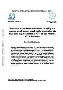
7. Background estimation The main SM background process in SRA−C, E, and F is Z → ν ν¯ production in association with heavy flavor jets. The second most dominant background is t t¯ production where one W decays via a lepton and neutrino and the lepton (particularly a hadronically decaying τ lepton) is either not identified or is reconstructed as a jet. This process is the major background contribution in SRD and an important background in SRB, SRC and SRE as well. Other important background processes are W → `ν plus heavy flavor jets, single top and the irreducible background from t t¯ + Z, where the Z decays to two neutrinos. The main background contributions are estimated primarily from comparisons between data and simulation. Control regions (CRs) are designed to enhance a particular source of background, and are orthogonal to the SRs while probing a similar event topology. The CRs are used to normalize the simulation to data, but the shape and extrapolation from the CR to the SR are taken from simulation. Sufficient data are needed to avoid large statistical uncertainties in the background estimates, and the CR definitions are chosen to be kinematically as close as possible to all SRs, to minimize the systematic uncertainties associated with extrapolating the background yield from the CR to the SR. Where CR definitions are farther from the SR definition, validation regions are employed to cross-check the extrapolation. In addition, control region selection criteria are chosen to minimize potential contamination from signal in the scenarios considered. The signal contamination is below 16% in all CRs for all signal benchmark points that have not been excluded by Run 1 searches. As the CRs are not 100% pure in the process of interest, the cross-contamination between CRs from other processes is estimated with simulated samples. The normalization factors and the cross contamination are determined simultaneously for all regions using a fit described below. Table 5 details the relative contribution for each SM background process as a function of the signal region, as well as the corresponding control region used to estimate that background contribution. Each control region may serve to estimate backgrounds from several signal regions. Normalization scale factors (SFs) for each background source are also presented. Detailed CR definitions are given in Table 6, and are defined of one or more leptons � � by the presence 0,1 miss that make them orthogonal with the signal regions. The ∆φ jet , ET , minimum mT (`, ETmiss ), and 0 mjet, R=1.2 requirements are designed to remove contamination from SM multijet processes (when defining these variables, only true jets are used, i.e. not the lepton). The number of leptons is indicated by N` and the transverse momentum of the lepton is indicated by pT` . In all one-lepton CRs, once the trigger and minimum pT` selection are applied, the lepton is treated as a non-b-tagged jet (as a stand-in for the hadronic τ leptons in the SRs) in the computation of all jet-related variables. In the two-lepton CRZ, the invariant mass of the two oppositely charged leptons, indicated by m`` , is selected to be consistent with the leptons having originated from a Z. These leptons are then vectorially added to the ETmiss to mimic the 0 Z → ν ν¯ decays in the SRs, forming the quantity ETmiss . Requirements such as the maximum mT (`, ETmiss ) and the minimum ∆R between the two highest-weight b-tagged jets and the lepton, ∆R (b, `) min , are used to enforce orthogonality. In CRST, the requirement on the invariant mass of the two highest-weight b-tagged jets, mbb , is used to reject t t¯ contamination from the control region enriched in single-top events. Distributions from the Z + jets and W + jets control regions (CRZ and CRW, respectively) are shown in Fig. 4, while Fig. 5 contains distributions from the t t¯ and single top quark control regions (CRT and CRT-ISR, and CRST, respectively). Contributions from all-hadronic t t¯ and multijet production are found to be negligible. These are estimated from data using a procedure described in detail in Ref. [67]. The procedure determines the jet response from simulated dijet events, and then uses this response function to smear the jet response in low-ETmiss
13
10
3
10
2
ATLAS Preliminary s=13 TeV, 13.3 fb-1 CRZ
Events / 40 GeV
Events / 40 GeV
104
Data SM Total Z tt Single Top
10
5
104
ATLAS Preliminary s=13 TeV, 13.3 fb-1 CRZ
Data SM Total Z tt
10
3
Single Top
tt+V
tt+V
W
W
102
Diboson
10
10
1
1
2.0
2.0
Data / SM
Data / SM
Diboson
1.5 1.0 0.5 0.0 0
200
400
1.5 1.0 0.5 0.0 0
600
p0 [GeV]
100
200
300
p3 [GeV]
T
T
104
10
3
10
2
(b)
ATLAS Preliminary s=13 TeV, 13.3 fb-1 CRZ
Events / 50 GeV
Events / 50 GeV
(a) Data SM Total Z tt Single Top
10
5
104
ATLAS Preliminary s=13 TeV, 13.3 fb-1 CRZ
Data SM Total Z tt
10
3
Single Top
tt+V
tt+V
W
W
102
Diboson
10
10
1
1
2.0
2.0
Data / SM
Data / SM
Diboson
1.5 1.0 0.5 0.0 0
200
400
600
800
1.5 1.0 0.5 0.0
1000
200
400
600
m bT,max’ [GeV]
10
(d)
ATLAS Preliminary s=13 TeV, 13.3 fb-1 CRW
Events / 40 GeV
Events / 50 GeV
(c) 104
Data SM Total W
3
tt Single Top
10
tt+V
2
104
10
3
10
2
ATLAS Preliminary s=13 TeV, 13.3 fb-1 CRW
Data SM Total W tt Single Top tt+V
Z
Z Diboson
10
10
1
1
2.0
2.0
Data / SM
Data / SM
Diboson
1.5 1.0 0.5 0.0 200
400
600
800
E miss T ’ [GeV]
800
1000
E miss T
1.5 1.0 0.5 0.0 0
100
200
[GeV]
300
p3 [GeV] T
(e)
(f) 0
Figure 4: Transverse momenta of (a) the leading-pT jet, (b) the fourth-leading-pT jet, (c) the mTb,max distribution, 0 and (d) the ETmiss distribution in CRZ, and (e) the ETmiss and (f) the transverse momentum of the fourth-leading-pT jet in CRW. The stacked histograms show the SM expectation, normalized using scale factors derived from the simultaneous fit to all backgrounds. The “Data/SM" plots show the ratio of data events to the total SM expectation. The hatched uncertainty band around the SM expectation and in the ratio plot illustrates the combination of MC statistical and detector-related systematic uncertainties. The rightmost bin includes all overflows.
14
ATLAS Preliminary s=13 TeV, 13.3 fb-1 CRT
Events / 50 GeV
Events / 25 GeV
200
Data SM Total tt Single Top
150
tt+V
10
3
ATLAS Preliminary s=13 TeV, 13.3 fb-1 CRT
Data SM Total tt Single Top tt+V
102
W
W
Z
100
Z
Diboson
Diboson
10
50
0 2.0
Data / SM
Data / SM
1
1.5 1.0 0.5 0.0
100
200
300
400
2.0 1.5 1.0 0.5 0.0 0
500
m 0jet, R =1.2 [GeV]
500
(b)
ATLAS Preliminary s=13 TeV, 13.3 fb-1 CRT-ISR
Events / 50 GeV
(a) Events / 0.1
1000
m bT,max [GeV]
Data SM Total tt Single Top
100
tt+V
ATLAS Preliminary s=13 TeV, 13.3 fb-1 CRT-ISR
Data SM Total tt Single Top
100
tt+V
W
W
Z
Z Diboson
50
50
0 2.0
0 2.0
Data / SM
Data / SM
Diboson
1.5 1.0 0.5 0.0 0
0.5
1.5 1.0 0.5 0.0 400
1
600
800
1000
RISR
(d)
ATLAS Preliminary s=13 TeV, 13.3 fb-1 CRST
Events / 50 GeV
Events / 50 GeV
3
Data SM Total Single Top tt
10
2
tt+V
10
3
ATLAS Preliminary s=13 TeV, 13.3 fb-1 CRST
Data SM Total Single Top tt
102
tt+V
W
W
Z
1
1
2.0
2.0
Data / SM
Data / SM
Z
10
Diboson
10
1.5 1.0 0.5 0.0 200
400
600
1400
pISR [GeV] T
(c)
10
1200
800
1000
Diboson
1.5 1.0 0.5 0.0 0
200
400
600
[GeV] E miss T
800
1000
m bT,min [GeV]
(e)
(f)
b,max 0 Figure 5: Distributions of (a) mjet, in CRT, (c) RISR and (d) pTISR in CRT-ISR, and (e) ETmiss and R=1.2 and (b) mT
(f) mTb,min in CRST. The stacked histograms show the SM expectation, normalized using scale factors derived from the simultaneous fit to all backgrounds. The “Data/SM" plots show the ratio of data events to the total SM expectation. The hatched uncertainty band around the SM expectation and in the ratio plots illustrates the combination of MC statistical and detector-related systematic uncertainties. The rightmost bin includes all overflows.
15
Table 5: Summary of control regions used to estimate the background contributions for each signal region. The percentages indicate the relative contribution of each background process; for example, SRA contains predominantly Z + jets and the normalization of the simulation is determined by data-MC comparison in CRZ. The ranges in percentages correspond to the variation across the signal subregions. The contributions may not total 100% since sub-dominant background contributions from t t¯ + W /Z, diboson, all-hadronic t t¯, and multijet processes are not listed. Normalization scale factors (SF) for each CR calculated from a simultaneous fit (described in 7) to all backgrounds in all the CRs are also presented; the given uncertainty is the combination of the corresponding MC statistical and detector-related systematic uncertainties.
Z + jets
t t¯
W + jets
single top
CRZ
CRT
CRT-ISR
CRW
CRST
SF
1.20±0.26
0.91±0.18
0.78±0.19
1.21±0.21
0.86±0.33
SRA
34%-58%
9%-14%
-
10%-11%
6%-9%
SRB
22%-42%
22%-25%
-
9%-13%
10%
SRC
37%-39%
6%-17%
-
18%-25%
20%-26%
SRD1-4
0%
-
91%-92%
2%
1%-4%
SRD5-8
2%-10%
-
70%-84%
5%-9%
4%-8%
SRE
38%
12%
-
8%
10%
SRF
32%
10%
-
12%
17%
seed events. The jet response is cross-checked with data where the ETmiss can be unambiguously attributed to the mis-measurement of one of the jets. Diboson and t t¯ + W /Z production, which is also sub-dominant, is estimated directly from simulation. Simultaneous fit to determine SM background The observed numbers of events in the various control regions are included in a profile likelihood fit [68] to determine the SM background estimates in each signal region. A likelihood function is built as the product of Poisson probability functions, describing the observed and expected number of events in the control regions [69]. This procedure takes common systematic uncertainties (discussed in detail in Section 8) between the control and signal regions and their correlations into account; they are treated as nuisance parameters in the fit and are modelled by Gaussian probability density functions. The free parameters in the fit are the overall normalizations of the backgrounds listed in Table 5. The contributions from all other background processes are fixed at the values expected from the simulation, using the most accurate theoretical cross sections available, as described in Section 4. The background estimates are validated by predicting the background in dedicated regions and comparing to observation. Validation regions are designed to be orthogonal to the control and signal regions while retaining kinematics and event composition close to the SRs but with little contribution from signal in any of the models considered. The Z + jets validation region are designed slightly differently in that they are subsets of the Z + jets control region which are still orthogonal to the signal regions.
16
Table 6: Selection criteria for the control regions used to estimate the background contributions in the signal regions.
Selection
CRZ
CRT
CRT-ISR
Trigger
electron (muon)
ETmiss
N`
2
1
pT`
CRST
CRW
> 20 GeV
m``
[86,96] GeV
-
Njet
≥4
≥ 4 (including leptons)
jet pT
(40, 40, 20, 20) GeV
ETmiss 0 ETmiss
< 50 GeV
> 250 GeV
> 70 GeV
-
b-tagged jets ∆φ �jet0,1, E miss � T
≥2
min mT (`, ETmiss )
-
30 GeV
-
30 GeV
30 GeV
max mT (`, ETmiss )
-
120 GeV
80 GeV
120 GeV
100 GeV
0 mjet, R=1.2 b,min mT
-
> 70 GeV
-
> 70 GeV
< 60 GeV
-
> 100 GeV
-
> 175 GeV
-
∆R (b, `) min
-
< 1.5
< 2.0
> 1.5
> 2.0
mbb
-
-
-
> 200 GeV
-
S Njet
-
-
≥5
-
-
S Nb-tag
-
-
≥1
-
-
pTISR
-
-
≥ 400 GeV
-
-
(80, 80, 40, 40) GeV
≥2
≥1
(80, 80, 20, 20) GeV
≥2
=1
> 0.4
-
17
8. Systematic uncertainties Several sources of experimental and theoretical systematic uncertainties are considered in the SM background estimates and signal expectations and are included in the profile likelihood fit described in Section 7. The dominant uncertainty to all SRs except for SRB-T0 is the statistical uncertainty on the mean estimate of the total background contribution. The main sources of detector-related systematic uncertainties in the SM background estimates originate from the jet energy scale (JES) and resolution (JER). The effect of the JES uncertainty on the background estimates in the signal regions is 1-4% in SRA and SRB, 1-5% in SRC, 2-9% in SRD, 5% in SRE and 2% in SRF. The uncertainty on the b-tagging efficiency has a large contribution as well. Its effect is 1-5% in SRA, 1-3% in SRB, 1-8% in SRC, 1-4% in SRD and is about 12% for SRE and 23% for SRF. Lepton reconstruction and identification uncertainties are also considered but have a small impact. All jet- and lepton-related uncertainties are propagated to the calculation of the ETmiss , and additional uncertainties on the energy and resolution of the soft term are also included. The uncertainty on the soft term of the ETmiss is most significant in SRD ranging between 1 and 10%, while being about 7% in both SRE and SRF. An uncertainty due to the pileup is also considered with a contribution in SRA of 1-6%, in SRB of 1-3%, in SRC of 1-2%, in SRD of 2-15%, in SRE of 3% and in SRF of 10%. A 2.9% uncertainty in the luminosity measurement is also taken into consideration for all signal and background estimates that are directly derived from MC simulations. Theoretical uncertainties in the modelling of the SM background are evaluated. For the W /Z + jets background processes, the modelling uncertainties are evaluated using SHERPA samples varying the renormalization and factorization scales, and the merging (CKKW) and resummation scales. The resulting impact on the total background yields from the Z + jets (W + jets) theoretical uncertainties are 7-12% (2%) for SRA, 4-9% (1-3%) for SRB, 8% (2-3%) for SRC, less than 1% for SRD, 8% (1%) for SRE and 7% (2%) for SRF. For the t t¯ background, uncertainties are evaluated due to the hard scattering generation (comparing MadGraph5aMC@NLO with Powheg-Box), the choice of the parton showering model (PYTHIA vs. HERWIG++) and the emission of additional partons in the initial and final states [46]. The largest impact of the t t¯ systematics on the total background yields arises for SRD and is about 22%, with lower contributions to SRC of 10%. For t t¯+W /Z background, the theoretical uncertainty is dominated by the 13% uncertainty on the production cross section. Additional variations considered include the choice of renormalization and factorization scales (each varied up and down by a factor of two). Uncertainty due to the choice of the generator is also considered comparing SHERPA at NLO with MadGraph5aMC@NLO. The single top background is dominated by the Wt subprocess. Uncertainties are evaluated for the choice of the parton showering model (PYTHIA vs. HERWIG++) and for the emission of additional partons in the initial and final state radiation. These uncertainties are about 10% in SRA and SRB, 17-25% in SRC, 10% in SRE and 16% in SRF. A 100% uncertainty is applied to account for the effect of interference between single-top quark and t t¯ production. Finally, signal systematic uncertainties due to detector and acceptance effects are taken into account when setting limits. The main sources of these uncertainties are the JER, ranging from 3 to 23%, the JES, ranging from 6 to 16% and pile-up, ranging from 6 to 20%. The uncertainty on the estimated number of signal events that arises from the cross section uncertainties for the various processes is taken into account by calculating two additional limits considering a ±1σ change in cross section. The cross section
18
uncertainty is ∼15% for direct top squark production, ∼30% for t t¯ production in association with two DM particles, and ∼20% for gluino production.
9. Results and interpretation The observed event yields in data are compared to the total number of expected background events in Tables 7, 8, 9, 10, and 11. The total background estimate is determined from the simultaneous fit based on a procedure described in Section 7. Figure 6 illustrates the distribution of the ETmiss and mTb,max combining the categories of SRA and SRB, respectively. The distribution of mTb,max in the most inclusive region of SRC, SRC-low, is shown in Fig. √ 7, while RISR is shown for the combined region of SRD1−4 and SRD5−8 miss in Fig. 8. Finally, the ET / HT and HT distributions for SRE and SRF, respectively, are presented in Fig. 9. In these figures, the background expectations are normalized to the values determined from the simultaneous fit. R Table 7: Expected and observed yields for SRA for L dt = 13.3 fb−1 .
SRA-TT Observed
8
Total SM t t¯
5.2 ± 1.4
W + jets Z + jets t t¯+W /Z Single top Dibosons Multijets
+ 0.84 − 0.78
0.78 0.48 ± 0.19 1.83 ± 0.55 1.03 ± 0.33 0.45 +− 0.53 0.45 0.62 ± 0.44 0.02 +− 0.05 0.02
SRA-TW
SRA-T0
5
16
5.7 ± 1.6
11.3 ± 2.6
0.60 ± 0.34 0.54 ± 0.18 3.0 ± 1.2 0.84 ± 0.26 0.34 +− 0.40 0.34 0.31 ± 0.20 0.01 +− 0.02 0.01
1.13 ± 0.79 1.13 ± 0.31 6.7 ± 2.1 1.29 ± 0.57 0.88 +− 0.97 0.88 0.18 ± 0.14 0.02 +− 0.05 0.02
No significant excess above the SM expectation is observed in any of the signal regions; the p-values, which express the probability that the background fluctuates to the data or above, and the model independent limits are shown in Table 12. The smallest p-values are 8%, 10%, and 13% for SRB-TT, SRC-low, and SRB-T0, respectively. In cases where the data fluctuate below the background the p-value is equal to 0.50 (e.g. SRD8). The 95% confidence level (CL) upper limits on the number of beyond-the-SM (BSM) events in each signal region are derived using the CLs prescription [70, 71] and calculated from asymptotic formulae [68]. Model-independent limits on the visible BSM cross sections, defined as σvis = σ · A · �, where σ is the production cross section, A is the acceptance, and � is the selection efficiency for a BSM signal, are reported. In addition to the individual p-values of each signal region, combined pvalues of 0.10 for both SRA and SRB are evaluated assuming the signal shape across categories of mt˜ = 800 GeV, m χ˜ 0 = 1 GeV and mt˜ = 600 GeV, m χ˜ 0 = 300 GeV, respectively. The detector acceptance multiplied by the efficiency (A· �) is calculated for several signal regions and their benchmark points. The A · � for signal regions aimed at high energy final states, SRA, SRE, SRF, ranges between 4.1% and 6.5% for their respective signal benchmark points of mt˜ = 800 GeV, m χ˜ 0 = 1 GeV,
19
R Table 8: Expected and observed yields for SRB for L dt = 13.3 fb−1 .
SRB-TT
SRB-TW
SRB-T0
Observed
17
18
84
Total SM t t¯
10.6 ± 2.3
16.7 ± 3.6
60
W + jets Z + jets t t¯+W /Z Single top Dibosons Multijets
2.5 ± 1.5 1.33 ± 0.35 2.40 ± 0.70 2.51 ± 0.64 1.1 +− 1.2 1.1 0.70 ± 0.44 0.06 +− 0.13 0.06
4.4 ± 2.6 1.44 ± 0.46 5.1 ± 1.6 3.15 ± 0.79 1.7 +− 1.9 1.7 0.87 +− 0.96 0.87 0.04 +− 0.08 0.04
± 14
14.7 ± 6.2 ± 26.0 ± 6.0 ± 6.1 −+ 1.33 ± 0.14 −+
4.4 1.5 8.8 1.4 6.7 6.1
0.75 0.29 0.14
R Table 9: Expected and observed yields for SRC, SRE, and SRF for L dt = 13.3 fb−1 .
SRC-low
SRC-med
SRC-high
SRE
SRF
Observed
36
14
9
9
3
Total SM t t¯
23.9 ± 7.5
9.4 ± 3.5
10.5 ± 3.7
7.1 ± 1.8
2.8 ± 1.0
0.92 ± 0.48 0.56 ± 0.17 2.78 ± 0.98 1.46 ± 0.55 0.70 +− 0.80 0.70 0.63 ± 0.48 0.02 0.01 −+ 0.01
0.32 ± 0.29 0.33 ± 0.12 0.92 ± 0.52 0.28 ± 0.11 0.46 +− 0.55 0.46 0.50 ± 0.31 0.01 +− 0.02 0.01
W + jets Z + jets t t¯+W /Z Single top Dibosons Multijets
4.4 ± 3.3 4.4 ± 1.3 9.5 ± 3.7 0.60 ± 0.21 4.5 +− 4.9 4.5 0.44 +− 0.66 0.44 0.09 +− 0.19 0.09
1.4 ± 1.3 1.85 ± 0.69 3.5 ± 1.6 0.19 ± 0.10 2.3 +− 2.5 2.3 0.07 ± 0.07 0.05 +− 0.11 0.05
0.72 ± 0.54 2.51 ± 0.57 4.0 ± 1.4 0.32 ± 0.14 2.7 +− 3.1 2.7 0.13 +− 0.30 0.13 0.04 +− 0.08 0.04
20
R Table 10: Expected and observed yields for SRD for L dt = 13.3 fb−1 .
SRD1
SRD2
SRD3
SRD4
Observed
4
5
9
9
Total SM t t¯
4.3 ± 1.9
7.1 ± 3.2
8.8 ± 3.4
9.4 ± 3.7
3.9 ± 1.9 0.14 +− 0.25 0.14 0.04 ± 0.02 0.11 ± 0.08 0.09 +− 0.14 0.09 −− 0.04 +− 0.08 0.04
6.5 ± 3.3 0.18 +− 0.27 0.18 0.06 ± 0.03 0.16 ± 0.12 0.19 +− 0.29 0.19 −− 0.04 +− 0.08 0.04
8.0 ± 3.4 0.24 +− 0.31 0.24 0.08 ± 0.06 0.20 ± 0.10 0.29 +− 0.57 0.29 −− 0.03 +− 0.06 0.03
8.5 ± 3.8 0.26 ± 0.20 0.08 +− 0.28 0.08 0.15 ± 0.13 0.42 +− 0.54 0.42 −− 0.02 +− 0.04 0.02
W + jets Z + jets t t¯+W /Z Single top Dibosons Multijets
R Table 11: Expected and observed yields for SRD for L dt = 13.3 fb−1 .
SRD5
SRD6
SRD7
SRD8
Observed
11
6
5
1
Total SM t t¯
11.6 ± 3.6
8.6 ± 3.5
5.2 ± 2.1
2.56 ± 0.86
6.8 ± 3.5 0.68 ± 0.23 0.23 +− 0.43 0.23 0.16 ± 0.11 0.48 +− 0.56 0.48 0.16 ± 0.11 0.02 +− 0.03 0.02
4.0 ± 2.0 0.37 ± 0.22 0.36 ± 0.13 0.08 +− 0.09 0.08 0.31 +− 0.35 0.31 0.16 ± 0.14 0.01 +− 0.01 0.01
1.77 ± 0.67 0.25 ± 0.18 0.30 ± 0.13 0.02 +− 0.02 0.02 0.22 +− 0.25 0.22 −− −−
W + jets Z + jets t t¯+W /Z Single top Dibosons Multijets
9.7 ± 3.7 0.68 ± 0.40 0.27 +− 0.52 0.27 0.26 ± 0.06 0.54 +− 0.64 0.54 0.16 ± 0.13 0.03 +− 0.06 0.03
21
Events / 100 GeV
Events / 50 GeV
15
Data
ATLAS Preliminary s=13 TeV, 13.3 fb-1 SRA
SM Total Z tt Single Top tt+V W Diboson ~ 0 (t ,∼ χ )=(800,1) GeV
10
1 1
ATLAS Preliminary s=13 TeV, 13.3 fb-1 SRB
40
Data SM Total Z tt Single Top tt+V
30
W Diboson ~ 0 (t ,∼ χ )=(600,300) GeV 1 1 0
~ (t1,∼ χ )=(600,250) GeV 1 ~ ± ∼0 (t1,∼ χ ,χ )=(600,400,200) GeV
20
1
1
5 10
0 200
400
600
800
miss ET
1000
0 0
500
[GeV]
1000
mbT,max [GeV]
Events / 100 GeV
Figure 6: Distributions of ETmiss for SRA and mTb,max for SRB. The categories have been combined in these distributions. The stacked histograms show the SM expectation and the hatched uncertainty band around the SM expectation shows the MC statistical and detector-related systematic uncertainties.
20 Data
ATLAS Preliminary s=13 TeV, 13.3 fb-1 SRC-low
SM Total Z tt
15
Single Top tt+V W Diboson ~ ± ∼0 (t ,∼ χ ,χ )=(400,100,50) GeV 1 1
1
1
1
~ ± ∼0 (t1,∼ χ ,χ )=(600,200,100) GeV 1 1 ~ ± ∼0 (t1,∼ χ ,χ )=(700,100,50) GeV
10
5
0 0
500
1000
mbT,max [GeV]
Figure 7: Distribution of mTb,max in SRC-low. The stacked histograms show the SM expectation and the hatched uncertainty band around the SM expectation shows the MC statistical and detector-related systematic uncertainties.
22
Events / 0.1
Events / 0.1
Data
ATLAS Preliminary s=13 TeV, 13.3 fb-1 SRD1-4
SM Total tt
10
Single Top tt+V
Data
ATLAS Preliminary s=13 TeV, 13.3 fb-1 SRD5-8
SM Total tt
10
Single Top tt+V W
W
Z
Z ~ 0 (t1,∼ χ )=(250,77) GeV 1 ~ 0 (t ,∼ χ )=(350,177) GeV
Diboson ~ 0 (t ,∼ χ )=(250,77) GeV 1 1
~ 0 (t1,∼ χ )=(350,177) GeV 1 ~ 0 (t1,∼ χ )=(450,277) GeV
1 1
~ 0 (t1,∼ χ )=(450,277) GeV 1
1
5
5
0 0
0.5
0 0
1
0.5
1
RISR
RISR
10
Data
ATLAS Preliminary s=13 TeV, 13.3 fb-1 SRE
SM Total Z tt Single Top tt+V W Diboson (ϕ,χ)=(350,1) GeV, g=3.5
Events / 200 GeV
Events / 2 GeV
Figure 8: Distributions of RISR for SRD1-SRD4 and SRD5-SRD8. The stacked histograms show the SM expectation and the hatched uncertainty band around the SM expectation shows the MC statistical and detector-related systematic uncertainties.
8
Data
ATLAS Preliminary s=13 TeV, 13.3 fb-1 SRF
SM Total Z tt Single Top
6
tt+V W Diboson ~~ (g,t1)=(1400,400) GeV
4
5
2
0
10
20
E miss T /
0 1000
30
1500
2000
2500
3000
H T [GeV]
H T [ GeV]
√ Figure 9: Distributions of ETmiss / HT for SRE and HT for SRF. The stacked histograms show the SM expectation and the hatched uncertainty band around the SM expectation shows the MC statistical and detector-related systematic uncertainties.
23
Table 12: Left to right: 95% CL upper limits on the visible cross section (h� σi95 ) and on the number of signal obs 95 95 events (Sobs ). The third column (Sexp ) shows the 95% CL upper limit on the number of signal events, given the expected number (and ±1σ excursions on the expectation) of background events. The two columns before last indicate the discovery p-value (p(s = 0)) and the the significance for the p-value (σ). The p-value is set to 0.50 when the observed event yield is less than the expected event yield.
h� σi95 [fb] obs
95 Sobs
95 Sexp
p(s = 0)
σ
SRA-TT
0.72
9.5
6.9+3.3 −2.1
0.18
0.92
SRA-TW
0.46
6.1
6.6+3.3 −2.0
0.50
0.00
0.16
0.99
0.08
1.41
0.41
0.23
0.10
1.28
0.13
1.13
0.19
0.88
0.50
0.00
0.50
0.00
0.50
0.00
0.49
0.03
0.50
0.00
0.50
0.00
0.50
0.00
0.49
0.03
0.50
0.00
0.29
0.55
0.47
0.08
Signal channel
SRA-T0
1.05
14.0
SRB-TT
1.17
15.5
SRB-TW
0.97
12.9
SRB-T0
3.91
52.1
SRC-low
2.19
29.1
SRC-med
1.10
14.6
SRC-high
0.66
8.8
SRD1
0.45
6.0
SRD2
0.47
6.2
SRD3
0.69
9.2
SRD4
0.67
8.9
SRD5
0.69
9.2
SRD6
0.50
6.6
SRD7
0.50
6.6
SRD8
0.28
3.7
SRE
0.72
9.5
SRF
0.42
5.6
24
10.1+4.4 −2.9 10.0+4.3 −2.9 12.1+4.8 −3.5 38.2+12.9 −10.0 21.9+7.4 −5.7 11.3+4.5 −3.2 +3.8 9.6−2.6 6.1+3.1 −2.0 7.6+3.1 −2.1 9.0+3.7 −2.7 9.2+3.8 −2.7 9.6+4.1 −2.8 8.1+3.6 −2.2 6.8+3.2 −1.9 4.7+2.6 −1.2 7.9+3.6 −2.3 5.4+2.6 −1.6
mϕ = 350 GeV, m χ = 1 GeV, and mg˜ = 1400 GeV, mt˜ = 400 GeV, m χ˜ 0 = 395 GeV. SRB and SRC-low have A · � of 1.2% and 1.3% for mt˜ = 600 GeV, m χ˜ 0 = 300 GeV and mt˜ = 700 GeV, m χ˜1± = 100, m χ˜ 0 = 50 GeV, respectively. Finally, SRD1-4 and SRD5-8 (combining the RISR windows) has an A · � of 0.12% and 0.22% for mt˜ = 350 GeV, m χ˜ 0 = 177 GeV and mt˜ = 450 GeV, m χ˜ 0 = 277 GeV. The profile likelihood ratio test statistic is used to set limits on direct pair production of top squarks. A fixed signal component is used, and any signal contamination in the CRs is taken into account. Again, limits are derived using the CLs prescription and calculated from asymptotic formulae. Orthogonal signal subregions, such as SRA-TT, SRA-TW, and SRA-T0, are statistically combined by multiplying their likelihood functions. A similar procedure is performed for the signal subregions in SRB. For the overlapping signal subregions defined for SRC and SRD, the signal subregion with the smallest expected 95% CLs value is chosen for each signal model. Once the signal subregions are combined or chosen, the signal region with the smallest expected 95% CLs is chosen from SRA, SRB, and SRD 0 for each signal model in the t˜- χ˜ 1 signal grid. The nominal event yield in each SR is set to the mean background expectation to determine the expected limits; contours that correspond to ±1σ uncertainties in the background estimates (σexp ) are also evaluated. The observed event yields determine the observed limits for each SR; these are evaluated for the nominal signal cross sections as well as for ±1σ theory SUSY . uncertainties on those cross sections σtheory Figure 10 (a) shows the observed R (solid red line) and expected (dashed blue line) exclusion limits at 95% 0 χ ˜ ˜ CL in the t - 1 mass plane for L dt = 13.3 fb−1 for SRA, SRB, and SRD. The data excludes top squark 0 masses in the range 310–820 GeV for χ˜ 1 masses below 160 GeV extending Run 1 limits by 100 GeV. Additional constraints are set in the case when mt˜ ∼ mt + m χ˜ 0 , for which top squark masses between 23–380 GeV are excluded. For signal models in the b- χ˜ 1 grid, the signal region with the smallest expected 95% CLs is chosen from SRB and SRC to yield the combined limit shown in Fig. 11. SRB is most sensitive in near the kinematic boundary of mt˜ = mb + m χ˜1± while SRC is the most sensitive along low m χ˜ 0 . Due to the mild excess in the number of observed events in SRB, the observed 95% CL limit is restricted to m χ˜1± values below 150 GeV while the expected limit extends to higher values. ±
The results for SRE are interpreted in terms of simplified models of top quarks produced in association with DM particles as a function of the DM and mediator masses, and varying coupling strengths (nominally g = 3.5). The exclusion limits on the m χ vs. mϕ and on the m χ vs. m a plane are shown in Fig. 12. In addition to showing limits assuming g = 3.5, Fig. 12 also contains upper limits on the coupling, g, indicated by the numbers on the figure, as a function of m χ and m a , mϕ . For both the scalar (pseudoscalar) interpretation the most stringent limits on the coupling are at low m χ and low mϕ (m a ). The SRF results are interpreted for indirect top squark production through gluino decays in terms of the χ˜ 01 vs. g˜ mass plane with ∆m(t˜, χ˜ 01 ) = 5 GeV. All grid points up to mg˜ = 1600 GeV with m χ˜ 0 < 560 GeV are excluded and upper limits on the g˜ pair production cross section are set and shown in Fig. 13.
25
m∼χ0 [GeV]
600
0 0 ~ Stop pair production, t1 → t ∼ χ1 / bW ∼ χ1
Observed limit (±1 σSUSY ) theory
ATLAS Preliminary
Expected limit (±1 σexp)
1
SRA+SRB+SRD
500
s=13 TeV, 13.3 fb-1 All limits at 95% CL
t
m
+
1
1
m
m + b
60 GeV
> 60 GeV
-
> 60 GeV
-
∆R (b, b)
-
> 0.8
> 0.8
> 0.8
-
mTb,max
-
> 100 GeV
> 200 GeV
> 100 GeV
-
HT √ ETmiss / HT
-
-
-
-
-
-
√ > 10 GeV
> 300 GeV √ > 8 GeV
0 mjet, R=0.8
-
-
-
-
> 30 GeV
The t t¯ background estimate is validated by defining several kinematic regions. In addition to the common all-hadronic preselection requirements, VRT-low (VRT-high) is required to have ETmiss > 250 GeV (ETmiss > 350 GeV) and is kinematically similar to SRB, SRC, and SRE (SRA and SRF). The events in VRT-low and VRT-high must have at least 2 b-tagged jets and an orthogonal mTb,min requirement: 50 < mTb,min < 150 GeV. Estimates of the t t¯ background contribution in SRD are validated using two regions: VRT-ISR1b and VRT-ISR-2b, which require at least 1 and at least 2 b-tagged jets, and correspond to SRD5-8 and SRD1-4, respectively. A requirement of RISR > 0.45 is applied to VRT-ISR-1b. For both regions, the S requirement is relaxed to N S ≥ 4, and the pjet 4,S MTS requirement is relaxed to MTS > 100 GeV, the Njet jet T requirement is removed. An additional requirement on the ratio of the transverse mass of the visible part of the sparticle system (MTS,Vis ) to MTS is imposed: MTS,Vis /MTS < 0.6 to reduce signal and multijet contamination. Finally, the pTISR requirement is inverted compared to the signal region; both validation regions require pTISR < 3.0. Data/simulation comparisons from VRT-low, VRT-high, VRT-ISR-1b, and VRT-ISR-2b are shown in Fig. 15. The background yield in each validation region is predicted from the combined fit to the control regions. The resulting estimate is consistent with the observed number of events in data; these results are
33
3
ATLAS Preliminary s=13 TeV, 13.3 fb-1 VRZA
Events / 2 GeV
Events / 40 GeV
10
Data SM Total Z tt
102
Single Top
10
3
ATLAS Preliminary s=13 TeV, 13.3 fb-1 VRZA
Data SM Total Z tt
102
Single Top
tt+V
1
1
2.0
2.0
1.5 1.0 0.5 0.0 0
200
400
Diboson
10
Data / SM
Data / SM
tt+V
Diboson
10
1.5 1.0 0.5 0.0
600
10
p0 [GeV]
20
10
3
(b)
ATLAS Preliminary s=13 TeV, 13.3 fb-1 VRZA
Events / 50 GeV
Events / 50 GeV
(a)
10
30 miss
E T ’/ H T [ GeV]
T
Data SM Total Z
2
tt Single Top
10
3
10
2
ATLAS Preliminary s=13 TeV, 13.3 fb-1 VRZA
Data SM Total Z tt Single Top
tt+V
tt+V
Diboson
1
1
2.0
2.0
1.5 1.0 0.5 0.0 0
200
400
600
800
1.5 1.0 0.5 0.0
1000
m bT,max’
Diboson
10
Data / SM
Data / SM
10
200
400
(d)
ATLAS Preliminary s=13 TeV, 13.3 fb-1 VRW
Events / 50 GeV
Events / 50 GeV
3
Data SM Total W tt
10
800
E miss T ’ [GeV]
(c)
10
600
[GeV]
Single Top
2
10
3
ATLAS Preliminary s=13 TeV, 13.3 fb-1 VRW
Data SM Total W tt
102
Single Top
tt+V
tt+V
Z
1
1
2.0
2.0
Data / SM
Data / SM
Z
10
Diboson
10
1.5 1.0 0.5 0.0 200
400
600
800
1000
Diboson
1.5 1.0 0.5 0.0 0
200
400
600
[GeV] E miss T
800
1000
m bT,min [GeV]
(e)
(f)
0 √ 0 Figure 14: Distributions of (a) pT of the leading jet, (b) ETmiss / HT , (c) mTb,max and (d) ETmiss in the VRZA, and (e) ETmiss and (f) the fourth-leading jet pT in VRW. The stacked histograms show the SM expectation, normalized using scale factors derived from the simultaneous fit to all backgrounds. The “Data/SM" plots show the ratio of data events to the total SM expectation. The hatched uncertainty band around the SM expectation and in the ratio plots illustrates the combination of MC statistical and detector-related systematic uncertainties. The rightmost bin includes all overflows.
34
ATLAS Preliminary s=13 TeV, 13.3 fb-1 VRT-low
Events / 50 GeV
Events / 25 GeV
600
Data SM Total tt Single Top
400
tt+V
104
10
3
ATLAS Preliminary s=13 TeV, 13.3 fb-1 VRT-high
Data SM Total tt Single Top tt+V
102
W
W
Z
Z
Diboson
Diboson
10
200
0 2.0
Data / SM
Data / SM
1
1.5 1.0 0.5 0.0
100
200
300
400
2.0 1.5 1.0 0.5 0.0 200
500
m 0jet, R =1.2 [GeV]
400
600
(b)
ATLAS Preliminary s=13 TeV, 13.3 fb-1 VRT-ISR-1b
Events / 50 GeV
Events / 50 GeV
10
1000
[GeV] E miss T
(a)
3
800
Data SM Total tt Single Top tt+V
102
W
10
3
ATLAS Preliminary s=13 TeV, 13.3 fb-1 VRT-ISR-2b
Data SM Total tt Single Top tt+V
102
W
Z
10
1
1
2.0
2.0
1.5 1.0 0.5 0.0 400
600
800
1000
Diboson
10
Data / SM
Data / SM
Z
Diboson
1200
1.5 1.0 0.5 0.0 400
1400
pISR [GeV]
600
800
1000
T
(d)
ATLAS Preliminary s=13 TeV, 13.3 fb-1 VRT-ISR-1b
Events / 0.1
Events / 0.05
1400
pISR [GeV] T
(c) 100
1200
Data SM Total tt Single Top
60
ATLAS Preliminary s=13 TeV, 13.3 fb-1 VRT-ISR-2b
SM Total tt Single Top
tt+V
tt+V
40
W
W
Z
50
Data
Z
Diboson
Diboson
0 2.0
Data / SM
Data / SM
20
1.5 1.0 0.5 0.0 0.4
0.6
0.8
1
0 2.0
1.5 1.0 0.5 0.0 0
0.5
RISR
1
RISR
(e)
(f)
0 Figure 15: Distributions of (a) mjet,R=1.2 in VRT-low, (b) ETmiss in VRT-high, (c) pTISR in VRT-ISR-1b , (d) pTISR VRTISR-2b, (e) RISR in VRT-ISR-1b, and (f) RISR in VRT-ISR-2b. The stacked histograms show the SM expectation, normalized using scale factors derived from the simultaneous fit to all backgrounds. The “Data/SM" plots show the ratio of data events to the total SM expectation. The hatched uncertainty band around the SM expectation and in the ratio plots illustrates the combination of MC statistical and detector-related systematic uncertainties. The rightmost bin includes all overflows.
35
summarized in Tables 14 and 15. Table 14: Event yields in the Z + jets validation regions compared to the background estimates obtained from the profile likelihood fit. Statistical and systematic uncertainties in the number of fitted background events are shown.
Observed Total SM t t¯ W + jets Z + jets t t¯+W /Z Single top Dibosons Multijets
VRZA 135 127 ± 31 0.80 ± 0.22 −− 119 ± 32 < 0.01 0.06 ± 0.04 6.8 ± 1.5 −−
VRZB 104 94 ± 23 0.80 ± 0.22 −− 89 ± 24 < 0.01 0.06 ± 0.04 4.6 ± 1.0 −−
VRZC 164 156 ± 36 0.75 ± 0.28 −− 148 ± 37 < 0.01 0.06 ± 0.05 8.0 ± 1.5 −−
VRZE 92 80 ± 20 0.54 ± 0.19 −− 76 ± 21 < 0.01 0.06 ± 0.04 3.66 ± 0.78 −−
VRZF 117 110 ± 26 0.61 ± 0.18 −− 103 ± 26 −− 0.06 ± 0.04 6.4 ± 1.2 −−
Table 15: Event yields in the t t¯ and W validation regions compared to the background estimates obtained from the profile likelihood fit. Statistical and systematic uncertainties in the number of fitted background events are shown.
Observed Total SM t t¯ W + jets Z + jets t t¯+W /Z Single top Dibosons Multijets
VRT-low 1735 1564 ± 350 1379 ± 330 40 ± 10 58 ± 17 22.9 ± 3.0 57 ± 24 5.1 ± 1.1 1.0 +− 2.1 1.0
VRT-high 345 330 ± 71 278 ± 65 11.3 ± 2.8 17.2 ± 4.5 6.32 ± 0.81 14.7 ± 6.3 2.06 ± 0.54 0.35 0.17 −+ 0.17
VRW 92 77 ± 14 15.8 ± 4.0 36.8 ± 8.6 0.16 ± 0.08 0.27 ± 0.05 23 ± 10 1.50 ± 0.26 −−
36
VRT-ISR-2b 270 199 ± 42 144 ± 40 14.0 ± 4.1 17.4 ± 4.2 6.1 ± 1.5 13.8 ± 5.3 1.98 ± 0.56 1.3 +− 2.7 1.3
VRT-ISR-1b 312 252 ± 58 158 ± 45 34 ± 11 32 ± 12 5.4 ± 1.4 16.5 ± 6.8 4.9 ± 2.6 0.7 +− 1.4 0.7
10−2
-1
s = 13 TeV, 13.3 fb (m~,m∼0) = (800,1) GeV
3.5
t
χ1
3 2.5
4
ATLAS Preliminary Simulation g
t
χ
1
3 2.5
10−3
2
10−3
2
1.5
1.5 −4
10
1
10−4
1
0.5 0 0
10−2
s = 13 TeV, 13.3 fb-1 (m~,m~,m∼0) = (1400,400,395) GeV
3.5
Events (1.0/N)dN
ATLAS Preliminary Simulation
∆R(W, b)
4
Events (1.0/N)dN
∆R(W, b)
A.2. Additional figures
0.5
200
400
600
800
1000
0 0
1200 1400 Top p [GeV]
200
400
600
800
T
1000
1200 1400 Top p [GeV] T
(a)
(b)
Figure 16: The true ∆R between the W and the b-quark vs. the true top pT in (a) simulated top squark pair 0 production with (t˜, χ˜ 1 ) = (800, 1) GeV and (b) simulated top squark production through gluino decays with 0 (g, ˜ t˜, χ˜ 1 ) = (1400, 400, 395) GeV. The common preselection criteria are applied with the exception of the b-jet requirement. The histograms are normalized to unity to illustrate the increased boost of the top quarks in the gluino-mediated top squark decays compared to direct top squark production.
37
Events / 25 GeV
Events / 50 GeV
ATLAS Preliminary s=13 TeV, 13.3 fb-1 VRT-low
104
Data SM Total tt Single Top
10
3
10
2
tt+V
ATLAS Preliminary s=13 TeV, 13.3 fb-1 VRT-high
100
Data SM Total tt Single Top tt+V
W
W
Z
Z
Diboson
Diboson
50
10
2.0
Data / SM
Data / SM
1
1.5 1.0 0.5 0.0 200
400
600
800
0 2.0
1.5 1.0 0.5 0.0
1000
100
200
300
[GeV] E miss T
(a)
400
500
m 0jet, R =1.2 [GeV]
(b)
Events / 50 GeV
Events / 40 GeV
0 Figure 17: Distributions of (a) ETmiss in VRT-low and (b) mjet, R=1.2 in VRT-high. The stacked histograms show the SM expectation, normalized using scale factors derived from the simultaneous fit to all backgrounds. The “Data/SM" plots show the ratio of data events to the total SM expectation. The hatched uncertainty band around the SM expectation and in the ratio plots illustrates the combination of MC statistical and detector-related systematic uncertainties. The rightmost bin includes all overflows.
Data
ATLAS Preliminary s=13 TeV, 13.3 fb-1 SRA
SM Total Z tt Single Top
10
tt+V W Diboson ~ 0 (t ,∼ χ )=(800,1) GeV
15
Data
ATLAS Preliminary s=13 TeV, 13.3 fb-1 SRA
SM Total Z tt Single Top tt+V W
10
Diboson ~ 0 (t ,∼ χ )=(800,1) GeV
1 1
1 1
5
0 0
5
100
200
300
0 0
400
m0jet, R =1.2 [GeV]
(a)
200
400
600
800
1000
mbT,min [GeV]
(b)
b,min 0 Figure 18: Distributions of (a) mjet, in SRA. The stacked histograms show the SM expectation R=1.2 and (b) mT and the hatched uncertainty band around the SM expectation shows the MC statistical and detector-related systematic uncertainties.
38
Events / 50 GeV
Events / 40 GeV
60
Data
ATLAS Preliminary s=13 TeV, 13.3 fb-1 SRB
SM Total Z tt Single Top tt+V W
40
Diboson ~ 0 (t ,∼ χ )=(600,300) GeV
60
Data
ATLAS Preliminary s=13 TeV, 13.3 fb-1 SRB
SM Total Z tt Single Top tt+V W
40
Diboson ~ 0 (t ,∼ χ )=(600,300) GeV
1 1
1 1
~ 0 (t1,∼ χ )=(600,250) GeV 1 ~ ± ∼0 (t1,∼ χ ,χ )=(600,400,200) GeV 1
~ 0 (t1,∼ χ )=(600,250) GeV 1 ~ ± ∼0 (t1,∼ χ ,χ )=(600,400,200) GeV
1
1
20
20
0 0
1
100
200
300
0 0
400
m0jet, R =1.2 [GeV]
200
400
(a)
600
800
1000
mbT,min [GeV]
(b)
Events / 50 GeV
Events / 0.4
b,min 0 Figure 19: Distributions of (a) mjet, in SRB. The stacked histograms show the SM expectation R=1.2 and (b) mT and the hatched uncertainty band around the SM expectation shows the MC statistical and detector-related systematic uncertainties.
Data
ATLAS Preliminary s=13 TeV, 13.3 fb-1 SRC-low
SM Total Z tt Single Top
20
tt+V W Diboson ~ ± ∼0 (t ,∼ χ ,χ )=(400,100,50) GeV 1 1
1
1
1
15
Data
ATLAS Preliminary s=13 TeV, 13.3 fb-1 SRC-low
SM Total Z tt Single Top tt+V W Diboson ~ ± ∼0 (t ,∼ χ ,χ )=(400,100,50) GeV
10
~ ± ∼0 (t1,∼ χ ,χ )=(600,200,100) GeV 1 1 ~ ± ∼0 (t1,∼ χ ,χ )=(700,100,50) GeV
1 1
1
1
1
~ ± ∼0 (t1,∼ χ ,χ )=(600,200,100) GeV 1 1 ~ ± ∼0 (t1,∼ χ ,χ )=(700,100,50) GeV
10 5
0 0
2
4
0 0
6
200
400
∆ R(b,b)
(a)
600
800
1000
mbT,min [GeV]
(b)
Figure 20: Distributions of (a) ∆R (b, b) and (b) mTb,min in SRC. The stacked histograms show the SM expectation and the hatched uncertainty band around the SM expectation shows the MC statistical and detector-related systematic uncertainties.
39
Events / 50 GeV
Events / 50 GeV
Data
ATLAS Preliminary s=13 TeV, 13.3 fb-1 SRD1-4
SM Total tt
6
Single Top tt+V W Z ~ 0 (t1,∼ χ )=(250,77) GeV 1 ~ 0 (t ,∼ χ )=(350,177) GeV
4
10
Data
ATLAS Preliminary s=13 TeV, 13.3 fb-1 SRD5-8
SM Total tt Single Top tt+V W Z Diboson ~ 0 (t ,∼ χ )=(250,77) GeV 1 1
1 1 ~ ∼0
~ 0 (t1,∼ χ )=(350,177) GeV 1 ~ 0 (t1,∼ χ )=(450,277) GeV
5
(t1,χ )=(450,277) GeV 1
1
2
0 400
600
800
1000
1200
0 400
1400
pISR [GeV]
600
800
1000
1200
1400
pISR [GeV]
T
T
(a)
(b)
8
Events / 50 GeV
Events / 40 GeV
Figure 21: Distributions of pTISR in (a) SRD1-4 and (b) SRD5-8. The stacked histograms show the SM expectation and the hatched uncertainty band around the SM expectation shows the MC statistical and detector-related systematic uncertainties.
Data
ATLAS Preliminary s=13 TeV, 13.3 fb-1 SRE
SM Total Z tt Single Top tt+V W
6
Diboson
Data
ATLAS Preliminary s=13 TeV, 13.3 fb-1 SRE
SM Total Z tt
6
Single Top tt+V W Diboson
(ϕ,χ)=(350,1) GeV, g=3.5
(ϕ,χ)=(350,1) GeV, g=3.5
4 4 2
2
0 0
100
200
300
0 200
400
m0jet, R =1.2 [GeV]
400
600
800
miss
ET
(a)
1000
[GeV]
(b)
0 miss in SRE. The stacked histograms show the SM expectation and Figure 22: Distributions of (a) mjet, R=1.2 and (b) ET the hatched uncertainty band around the SM expectation shows the MC statistical and detector-related systematic uncertainties.
40
Events / 50 GeV
Events / 2 GeV
4
Data
ATLAS Preliminary s=13 TeV, 13.3 fb-1 SRF
SM Total Z tt Single Top
3
tt+V W Diboson ~~ (g,t1)=(1400,400) GeV
4
Single Top
Diboson ~~ (g,t1)=(1400,400) GeV
1
30
E miss T /
0
40
tt+V W
1
20
Z tt
2
10
SM Total
3
2
0
Data
ATLAS Preliminary s=13 TeV, 13.3 fb-1 SRF
500
1000
H T [ GeV]
miss
ET
(a)
1500
[GeV]
(b)
√ Figure 23: Distributions of (a) ETmiss / HT and (b) ETmiss in SRF. The stacked histograms show the SM expectation and the hatched uncertainty band around the SM expectation shows the MC statistical and detector-related systematic uncertainties.
41