Attractor networks for shape recognition
Yali Amit
2
and Massimo Mascaro
1
3
Abstract We describe a system of thousands of binary perceptrons with coarse oriented edges as input which is able to successfully recognize shapes, even in a context with hundreds of classes. The perceptrons have randomized feedforward connections from the input layer and form a recurrent network among themselves. Each class is represented by a pre-learned attractor (serving as an associative ‘hook’) in the recurrent net corresponding to a randomly selected subpopulation of the perceptrons. In training first the attractor of the correct class is activated among the perceptrons, then the visual stimulus is presented at the input layer. The feedforward connections are modified using field dependent Hebbian learning with positive synapses, which we show to be stable with respect to large variations in feature statistics and coding levels, and allows the use of the same threshold on all perceptrons. Recognition is based only on the visual stimuli. These activate the recurrent network, which is then driven by the dynamics to a sustained attractor state, concentrated in the correct class subset, and providing a form of working memory. We believe this architecture is on one hand more transparent than standard feedforward two layer networks and on the other hand has stronger biological analogies.
1 Appeared:
Neural Computation, vol. 13, pp. 1415-1442, 2001 of Statistics, University of Chicago, Chicago, IL, 60637; Email:
[email protected]. Supported in part by the Army Research Office under grant DAAH04-96-1-0061 and MURI grant DAAH04-96-1-0445, 3 Department of Statistics, University of Chicago, Chicago, IL, 60637; Email:
[email protected]. Supported by NSF-GIG DSM97-09696. 2 Department
1
Introduction
Learning and recognition in the context of neural networks is an intensively studied field. The leading paradigm from the engineering point of view is that of feed-forward networks. To cite only a few examples in the context of character recognition, see (LeCun et al., 1990), (Knerr et al., 1992), (Bottou et al., 1994), (Hussain & Kabuka, 1994). Two layer feed-forward networks have proved to be very useful as classifiers in numerous other applications. However they lack a certain transparency of interpretation relative to decision trees, for example, and their biological relevance is quite limited. Learning is not Hebbian and local, rather it employs gradient descent on a global cost function. Furthermore these nets fail to address the issue of sustained activity needed to deal with working memory. On the other hand much work has gone into networks in which learning is Hebbian, and recognition is represented through the sustained activity of attractor states of the network dynamics. See (Hopfield, 1982), (Amit, 1989), (Amit & Brunel, 1995), (Brunel et al., 1998). In this field however research has primarily focused on the theoretical and biological modeling aspects. The input patterns used in these models are rather simplistic, ‘easy’, from the statistical point of view. The prototypes for each class are assumed uncorrelated with approximately the same coding level. The patterns for each class are assumed to be simple noisy versions of the prototypes, with independent flips of low probability at each feature. These models have so far avoided the issue of how the attractors can be used for classification of real data, for example image data, where the statistics of the input features are more complex. Indeed if the input features of visual data are assumed to be some form of local edge filters, or even local functions of these edges, there is a very significant variability in conditional distributions of these features given each class. This is described in detail in section 4.1. In this paper we make an attempt to bridge the gap between these two rather disjoint fields of research yet trying to minimize the assumptions we make regarding the information encoded in individual neurons or in the connecting synapses, as well as staying faithful to the idea that learning is local. Thus the neurons are all binary and all have the same threshold. Synapses are positive with a limited range of values and can be effectively assumed binary. The network can easily be modified to have multi-valued neurons - the performance would only improve. However since it is still unclear to what extent the biological system can exploit the fine details of neuronal firing rates or spike timing we prefer to work with binary neurons essentially representing high and low firing rates. Similar considerations hold for the synaptic weights, moreover the work in (Petersen et al., 1998) suggests that potentiation in synapses is indeed discrete. The network consists of a recurrent layer A with random feed forward connections from a visual input layer I. Attractors are trained in the A layer, in an unsupervised way, using K classes of easy stimuli, namely noisy versions of K uncorrelated prototypes represented by subsets Ac , c = 1, . . . , K, in which the neurons are on. The activities of the attractors are concentrated around these subsets. Each visual class is then arbitrarily associated to one of the easy stimuli classes and is hence represented by the subset or population Ac . Prior to the presentation of visual input from class c to layer I a noisy version of the easy stimulus associated to class c is used to drive the recurrent layer to an attractor state so that activity concentrates in the population Ac . Following this the feedforward connections between layers I and A are updated. This stage of learning is therefore supervised. The easy stimuli are not assumed to reach the A layer via the visual input layer I. They can be viewed for example as reward type stimuli arriving from some other pathway (auditory, olfactory, tactile) as described in (Rolls, 2000), potentiating cues described in (Levenex & Schenk, 1997) or ‘mnemonic’ hooks introduced in (Atkinson, 1975). In testing only visual input is presented at layer I. This leads to the activation of certain units in A, and the recurrent dynamics leads this layer to a stable state which hopefully concentrates on the population corresponding to the correct class. All learning proceeds along the Hebbian paradigm. A continuous internal synaptic state increases 1
when both pre and post-synaptic neurons are on (potentiation), and decreases if the pre-synaptic neuron is on but the post synaptic neuron is off (depression). The internal state translates through a binary or sigmoidal transfer function to a synaptic efficacy. We add one important modification. If at a given presentation the local input to a post-synaptic neuron is above a threshold (higher than the firing threshold) the internal state of the afferent synapses does not increase. This is called field dependent Hebbian learning. This modification allows us to avoid global normalization of synaptic weights or the modification of neuronal thresholds. Moreover field dependent Hebbian learning turns out to be very robust to parameter settings, avoids problems due to variability in the feature statistics in the different classes, and does not require apriori knowledge of the size of the training set or the number of classes. The details of the learning protocol and its analysis are presented in section 4. Note that we are avoiding real time dynamic architectures involving noisy integrate and fire neurons and real time synaptic dynamics as in (Amit & Brunel, 1995), (Mattia & Del Giudice, 1999), (Fusi et al., 1999), and are not introducing inhibition. In future work we intend to study the extension of these ideas to more realistic continuous time dynamics. The visual input has the form of binary oriented edge filters with eight orientations. The orientation tuning is very coarse so that these neurons can be viewed as having a flat tuning curve spanning a range of angles as opposed to the classical bell shaped tuning curves. Partial invariance is incorporated by using complex type neurons, which respond to the presence of an edge within the range of orientations anywhere in a moderate size neighborhood. This type of partially invariant unit which responds to a disjunction (union) or a local MAX operation has been used in (Fukushima, 1986), (Fukushima & Wake, 1991), in (Amit & Geman, 1997), (Amit & Geman, 1999), (Amit, 2000), and recently in (Riesenhuber & Poggio, 1999). From a purely algorithmic point of view the attractors are unnecessary. Activity in the A layer can be clamped to the set Ac during training, and testing can simply be based on a vote in the A layer. In fact the attractor dynamics applied to the visual input leads to a decrease in performance as explained in section 3.2. However from the point of view of neural modeling the attractor dynamics is appealing. In the training stage it is a robust way to assign a ‘label’ to a class without pin-pointing a particular individual neuron. In testing the attractor dynamics ‘cleans’ the activity in layer A it is concentrated within a particular population which again corresponds to the ‘label’. This could prove useful for other modules which need to read out the activity of this system for subsequent processing stages. Finally the attractor is a stable state of the dynamics and is hence a mechanism for maintaining a sustained activity representing the recognized class, i.e. working memory, as in (Miyashita & Chang, 1988), (Sakai & Miyashita, 1991). We have chosen to experiment with this architecture in the context of shape recognition. We work with the NIST hand-written digit dataset, and a dataset of 293 randomly deformed LATEX symbols, which are presented in a fixed size grid although they exhibit significant variation in size as well as other forms of linear and non-linear deformation. In figure 10 we display a sample from this data set. With one network with 2000 neurons in the A layer we achieve 94% classification rate on NIST (see section 5). We believe this is very encouraging given the constrained learning and encoding framework we are working with. Moreover a simple boosting procedure whereby several nets are trained in sequence brings the classification rate to 97.6%. Although far from the best reported in the literature, which is over 99% (see (Wilkinson et al., 1992), (Bottou et al., 1994), (Amit et al., 1997)), this is definitely comparable to many experimental papers on this subject such as (Hastie et al., 1995), and (Avimelelch & Intrator, 1999) where boosting is also employed. The same holds for the LATEX database where the only comparison is with respect to decision trees studied in (Amit & Geman, 1997). Boosting consists of training a new network on training examples which are misclassified by the combined vote of the existing networks. The concept of boosting is appealing in that hard examples are put aside for further training and processing. In this paper however we do
2
not describe explicit ways to model the actual neural implementation of boosting. Some ideas are offered in the discussion section. The paper is organized as follows. In section 2 we discuss related work, similar architectures, learning rules, and the relation to certain ideas in the machine learning literature. In section 3 the precise architecture is described as well as the learning rule and the training procedure. In section 4 we analyze this learning rule and compare it to standard Hebbian learning. In section 5 we describe experimental results on both data sets and study the sensitivity of the learning rule to various parameter settings.
2 2.1
Related work Architecture
The architecture we propose consists of a visual input layer feeding into an attractor layer. The main activity during learning involves updating the synaptic weights of the connections between the input layer and the attractor layer. Such simple architectures have recently been proposed both in (Riesenhuber & Poggio, 1999) and in (Bartlett & Sejnowski, 1998). In (Riesenhuber & Poggio, 1999) the second layer is a classical output layer with individual neurons coding for different classes. No recurrent activity is modeled either during training or testing, but training is supervised. The input layer codes large range disjunctions, or MAX operations, of complex features which are in turn conjunctions of pairs of ‘complex’ edge type features. In an attempt to achieve large range translation and scale invariance, the range of disjunction is the entire visual field. This means that objects are recognized based solely on the presence or absence of the features, entirely ignoring their location. With sufficiently complex features this may well be possible, but then the combinatorics of the number of necessary features appears overwhelming. It should be noted that in the context of character recognition studied here we find a significant drop in classification rates when the range of disjunction or maximization is on the order of the image size. This tradeoff between feature complexity, combinatorics, and invariance is a crucial issue which has yet to be systematically investigated. In the architecture proposed in (Bartlett & Sejnowski, 1998) the second layer is a recurrent layer. The input features are again edge filters. Training is semi-supervised, not directly through the association of certain neurons to a certain class, but through the sequential presentation of slowly varying stimuli of the same class. Hebbian learning of temporal correlations is used to increase the weight of synapses connecting units in the recurrent layer responding to these consecutive stimuli. At the start of each class sequence the temporal interaction is suspended. This is a very appealing alternative to supervision which employs the fact that objects are often observed by slowly rotating them in space. This network employs continuous valued neurons and synapses, which can in principle achieve negative values. A bias input is introduced for every output neuron, which corresponds to allowing for adaptable thresholds, and depends on the size of the training set. Finally the feed-forward synaptic weights are globally normalized. It would be interesting to study whether field dependent Hebbian learning can lead to similar results without use of such global operations on the synaptic matrix.
2.2
Field dependent Hebbian learning
The learning rule employed here is motivated on one hand by work on binary synapses in (Amit & Fusi, 1994), (Amit & Brunel, 1995), (Mattia & Del Giudice, 1999), where the synapses are modified stochastically only as a function of the activity of the pre and post synaptic neurons. Here however
3
we have replaced the stochasticity of the learning process with a continuous internal variable for the synapse. This is more effective for neurons with a small number of synapses on the dendridic tree. On the other hand we draw from (Diederich & Opper, 1987), where Hopfield type nets with positive and negative valued multi-state synapses are modified using the classical Hebbian update rule, but modification stops when the local field is above or below certain thresholds. There exists ample evidence for local synaptic modification as a function of the activities of pre and post-synaptic neurons, (Markram et al., 1997), (Bliss & Collingridge, 1993). However at this point we can only speculate whether this process can be controlled by the depolarization or the firing rate of the post-synaptic neuron. One possible model in which such controls may be accommodated can be found in (Fusi et al., 2000).
2.3
Multiple classifiers
From the learning theory perspective, the approach we propose is closely related to current work on multiple classifiers. The idea of multiple randomized classifiers is gaining increasing attention in the machine learning theory, see (Amit & Geman, 1997), (Breiman, 1998), (Breiman, 1999), (Dietterich, 1998), (Amit et al., 1999). In the present context each unit in layer A associated to a class c is a randomized perceptron classifying class c against the rest of the world, and the entire network is an aggregation of multiple randomized perceptrons. Population coding among a large number of such linear classifiers can produce very complex classification boundaries. It is important to note however that the family of possible perceptrons available in this context is very limited due to the constraints imposed on the synaptic values and the use of uniform thresholds. A complementary idea is that of boosting where multiple classifiers are created sequentially by up-weighting the misclassified data points in the training set. Indeed in our context, to stabilize the results produced using the attractors in layer A and to improve performance, we train several nets sequentially using a simplified version of the boosting proposed in (Schapire et al., 1998), (Breiman, 1998).
3
The network
The network is composed of two layers, layer I for the visual input, and a recurrent layer A where attractors are formed and population coding occurs. Since it is still unclear to what extent biological systems can exploit the fine details of neuronal firing rates or spike timing we prefer to work with binary 0/1 neurons, essentially representing high and low firing rates. The I layer has binary units i = (x, e) for every location x in the image and every edge type e = 1, . . . , 8 corresponding to eight coarse orientations. Orientation tuning is very coarse so that these neurons can be viewed as having a flat tuning curve spanning a range of angles as opposed to the classical bell shaped tuning curves. The unit (x, e) is ‘on’ if an edge of type e has been detected anywhere in a moderate size neighborhood (anywhere between 3×3 and 10×10) of x. In other words a detected edge is ‘spread’ to the entire neighborhood. Thus these units are the analogs of ‘complex’ orientation sensitive cells (Hubel, 1988). In figure 1 we show an image of a ‘0’ with detected edges and the units that are activated after ‘spreading’. We emphasize that recognition does not require careful normalization of the image to a fixed size. Observe for example the significant variations in size and other shape parameters of the samples in the bottom panel of figure 10. Therefore the ‘spreading’ of the edge features is crucial for maintaining some invariance to deformations, and significantly improves the generalization properties of any classifier based on oriented edge inputs. The attractor layer has a large number of neurons NA , on the order of thousands, with randomly assigned recurrent connections allocated to each pair of neurons with probability pAA . The feedforward connections from I to A are also independently and randomly assigned with probability pIA 4
Figure 1: Top from left to right: Example of a deformed LATEX ‘0’. Detected edges of angle 0, edges of angle 90, edges of angle 180, edges of angle 270 (note that the edges have a polarity). Bottom from left to right: same edges spread in a 5 × 5 neighborhood.
Layer A
Layer I Figure 2: An overview of the network. There are two layers, denoted I and A. Units in layer A receive inputs from a random subset of layer I and from other units in layer A itself. Dashed arrows represent input from neurons in I, solid ones from neurons in A. for each pair of neurons in I and A respectively. This system of connections is described figure 2. Each neuron a ∈ A receives input of the form ha = hIa + hA a =
NI X
Eia ui +
NA X
Ea0 a ua0 ,
(1)
a0 =0
i=0
where ui , ua represent the states of the corresponding neurons, and Eia , Ea0 a are the efficacies of the connecting synapses. The efficacy is assumed 0 if no synapse is present. The input ha is also called the local field of the neuron, and decomposes into the local field due to feedforward input hIa , and the local field due to the recurrent input - hA a . The neurons in A respond to their input field through a step function: ua = Θ(ha − θ) (2) 5
10 Jm
Efficacy
8 6 4 2 0 0
L 50
H 100
150
200
250
Status Figure 3: The transfer function for converting the internal state of the synapse to its efficacy. The function is 0 below L, and saturates at Jm above H. In between it is linear. 0 and 255 are reflecting barriers for the status. In this example L=50, H=150, Jm = 10.
where
( Θ(x) =
1 for x > 0 0 for x ≤ 0
.
(3)
All neurons are assumed to have the same firing threshold θ, they are all excitatory and are updated asynchronously. Inhibitory neurons could be introduced in the attractor layer to perhaps stabilize or to create competition among the attractors. Each synapse is characterized by an internal state variable S. This state has two reflecting barriers forcing it to stay in the range [0, 255]. The efficacy E is a deterministic function of the state. This function is the same for all synapses of the net: E(S) = 0 for S ≤ L S−L (4) E(S) = H−L Jm for L < S < H E(S) = Jm for S ≥ H The parameter L defines the minimal state at which the synapse is activated, and H defines the state at which the synapse is saturated. Varying L and H produces a broad range of synapse types, from binary synapses when L = H, to completely continuous ones in the allowed range (L = 0, H = 255). The parameter Jm represents the saturation value of the efficacy. A graphical explanation of these parameters is provided in figure 3.
3.1
Learning
Given a pre-synaptic unit s and a post-synaptic unit t the synaptic modification rule is of the form ∆Sst = C+ (ht )us ut − C− (ht )us (1 − ut )
6
(5)
where: C+ (ht ) = Cp Θ(θ(1 + kp ) − ht ),
(6)
C− (ht ) = Cd Θ(ht − θ(1 − kd )).
(7)
Typically kp ranges between .2 and .5 and kd ≤ 1. In our experiments Cd is fixed to 1 while Cp ranges from 4 to 10. In regular Hebbian learning whenever both the pre and post-synaptic neurons are on the internal state increases, and whenever the pre-synaptic neuron is on and the post-synaptic neuron is off the internal state decreases. In other words the functions C+ and C− do not depend on the local field and are held constant at Cp and Cd respectively. The effect of the proposed learning rule is to stop synaptic potentiation when the input to the post-synaptic neuron is too high (higher than θ(1 + kp )) or to stop synaptic depression when the input is too low (less than θ(1 − kd )). Of course once a different input is presented the field changes and potentiation or depression may resume. The parameters kp (potentiation) and kd (depression) regulate to what degree the field is allowed to differ from the firing threshold before synaptic modification is stopped. These parameters may vary for different types of synapses. For example the recurrent synapses versus the feedforward ones. The parameters Cp and Cd regulate the amount of potentiation and depression applied to the synapse when the constraints on the field are satisfied. The transfer from internal synaptic state to synaptic efficacy needs to be computed at every step of learning in order to calculate the local field ha of the neuron in terms of the actual efficacies. This learning rule bears some similarities to the perceptron rule (Rosenblatt, 1962), to the field dependent rules proposed by (Diederich & Opper, 1987), and to the penalized weighting in (Oja, 1989). However it is implemented in the context of binary 0/1 neurons and non-negative synapses. In some experiments synapses have been constrained to be binary with a small loss in performance. The main purpose of field constraints on synaptic potentiation is to keep the average local field for any unit a ∈ A to be approximately the same, irrespective of the specific distribution of feature probabilities for the class represented by a. This enables the use of a fixed threshold for all neurons in layer A. In contrast to regular Hebbian learning this form of learning is not entirely local at the synaptic level due to the dependence on the field of the neuron. However if continuous spiking units were employed the field constraints could be reinterpreted as a firing rate constraint. For example, when the post-synaptic neuron fires at a rate above some level, which is significantly higher than the rate determined by the recurrent input alone, potentiation of any incoming synapses ceases. It should also be noted that the role of the internal synaptic state is to slow down synaptic modifications similar to the idea of stochastic learning in (Brunel et al., 1998) and (Amit & Brunel, 1995). A more detailed discussion of the properties of this learning rule is provided in section 4. Learning the recurrent efficacies We assume that the A layer receives noisy versions of K uncorrelated prototypes from some external source. These are well separated, ‘easy’, stimuli which are associated to the different visual classes. Although they are well separated we still expect some noise to occur in their activation. Specifically, we include each unit in A independently with probability pA in each of K subsets Ac . Each of these random subsets defines a prototype - all neurons in the subset Ac are on and all in its complement are off. The subsets belonging to each class p will be of different size, fluctuating around an average of pA NA units with a standard deviation of pA (1 − pA )NA . A typical case for a small NIST classifier, as in section 5, would be NA = 200 and pA = .1, so that the number of units in each class will be 20 ± 4. Random overlaps, namely units belonging to more than one subset, are significant. For example, in the case above about 60% of the units of a subset will also belong to other subsets. Given a noise level f (say 5 − 10%), a random stimulus from class c will have each neuron in Ac on with probability 1−f and each neuron in the complement of Ac on with probability f . Thus the sets 7
Layer I
Layer A
Class1
Layer A
Class 2
Layer I Figure 4: Left: a global view of layers I and A, emphasizing that the subsets in A are random and unordered. Each class is represented by a different symbol. Right: A closeup showing the input features extracted in I, random connections between the layers, recurrent connections in A, and possible overlaps between subsets in A. Ac correspond to prototype patterns and the actual stimuli are noisy versions of these prototypes. The recurrent synapses in A are modified by presenting random stimuli from the different classes in random order. Modification proceeds as prescribed in equation 5. After a sufficient number of presentations this network will develop attractors corresponding to the subsets Ac with certain basins of attraction. Moreover whenever the net is in one of these attractor states the average field on each neuron in a subset Ac will be approximately θ(1 + kp ). Note that the fluctuations in the size of the sets Ac typically reduce the maximum memory capacity of the network , see (Brunel, 1994). We use subsets of several tens of neurons so that pA is very small. Figure 4 provides a graphic description of the way the different populations are organized. We re-emphasize that direct learning of attractors on the visual inputs of highly variable shapes is impossible due to the complex structure of the statistics of the input features. Large overlaps exist between classes and coding levels vary significantly. Learning the feed forward efficacies Once the attractors in layer A have been formed learning of the feedforward connections can begin. Preceding the presentation of the visual input of a data point from class c to layer I the corresponding external input (again with noise) is presented to A and the associated attractor state emerges, with activity concentrated around the subset Ac . Learning then proceeds by updating the synaptic state variables Sia between layers I and A according to the field learning rule. Note that the field at a unit a ∈ A is composed of hIa and hA a . However since we assume that at this stage of learning the A layer is in an attractor state, the field hA a is approximately θ(1 + kp ) and we rewrite the learning rule for the feedforward synapses only in terms of the feed-forward local field hIa ∆Sia = C+ (hIa )ua ui − C− (hIa )(1 − ua )ui , (8) where a ∈ A has a connection from i ∈ I, and C+ (hIa ) = Cp Θ(θ(1 + kp ) − hIa ),
(9)
C− (hIa ) = Cd Θ(hIa − θ(1 − kd )),
(10)
8
using the same parameters kp , kd as in the recurrent synapses. This same rule can be written in terms of the entire field ha , if the value of kp on the feedforward connections is modified to kp0 = 2kp + 1. Whereas for recurrent synapses potentiation stops when the local field is above θ(1 + kp ), for feedforward synapses potentiation stops when the local field is above θ(1 + kp0 ) = θ(2 + 2kp ).
3.2
Recognition
Testing and the role of the attractors After training the feed-forward and recurrent synapses are held fixed and testing can be performed. A pattern is presented only at the input level I. The activity of the neurons in this layer creates direct activation in some of the neurons in layer A. First it is possible to carry out a simple majority vote among the classes, i.e. how many neurons were activated in each of the subsets Ac . This yields a classification rule, which corresponds to a population code for the class. The architecture is then nothing but a large collection of randomized perceptrons each trained to discriminate between one class, or several classes (in the case where a unit in layer A happens to be selective to several classes,) against the ‘rest of the world’, namely all other classes merged together as one. Recall that synaptic connections from layer I to A are chosen randomly. For each pair i ∈ I, a ∈ A the connection is present independently with probability pIA , (which may vary between 5 to 50 percent.) This randomization ensures that units assigned to the same class in layer A produce different classifiers based on different subsets of features. The performance of this scheme is surprisingly good given the simplicity of the architecture and of the training procedure. For example on the feed-forward nets with 50000 training and 50000 test samples on the NIST database we have observed a classification rate of 94%. When recurrent dynamics are applied to layer A, initialized by the direct activation produced by the feedforward connections, we obtain convergence to an attractor state which serves as a mechanism for working memory. Moreover the activity is concentrated on the recognized class alone. This is a non-trivial task since the noise around the actual subset Ac produced by the bottom up input can be very substantial, and is not at all the same as the independent f -level noise used to train the attractors. The classification rates with the attractors on an individual net are therefore often lower than voting based on the direct activation from the feed-forward connections. In some cases the response to a given stimulus is lower than usual and not enough neurons are activated in any of the classes to reach an attractor. Alternatively a stimulus may produce a strong enough response in more than one class producing a stable state composed of a union of attractors. In both cases the outcome after the net converges to a stable state could be wrong even if the initial vote was correct. One more source of noise on the attractor level lies in the overlap between the populations Ac in the A layer.
3.3
Boosting
A popular method to improve the performance of any particular form of classification is boosting, see for example (Schapire et al., 1998). The idea is to produce a sequence of classifiers using the same architecture and the same data. At each stage the sequence of classifiers is aggregated and produces an outcome based on voting among the classifiers. Furthermore at each stage those training data points which remain misclassified are up-weighted. A new classifier is then trained using the new weighting of the training set. In the extreme case each new classifier is constructed only from the misclassified training points of the current aggregate. We employed this extreme version for simplicity.
9
More precisely assume k nets A1 , . . . , Ak have been trained, each one with a separate attractor layer, and synaptic connections to the the same input layer I. The aggregate classifier of the k nets is the vote among all neurons in the k attractor layers. Only the misclassified training points of this aggregate net are used to train the k + 1 net. After net Ak+1 is trained, both in terms of the recurrent connections and the feedforward connections, it joins the pool of the k existing networks for voting. Note that voting is not weighted, all neurons in all Ak layers have equal vote. Examples of classification with boosting are given in section. 5.
4
Field learning
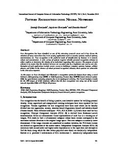
In this section we study the properties of field learning on the feed forward connections in greater detail. Henceforth the field refers only to the contribution of the input layer, i.e. hIa . Recall that each feature i = (x, e) is on if an edge of type e is present somewhere in a neighborhood of x. For each i and class c let pi,c denote the probability that ui = 1 for images in class c and qi,c the probability that ui = 1 for images not in class c. Let P (c), c = 1 . . . , K denote the prior on class c, namely the proportions of the different classes, and let p˜i,c = pi,c P (c), q˜i,c = qi,c (1 − P (c)). Finally let p˜i,c ρi,c = . (11) q˜i,c For the type of features we are employing in this context, and in many other real world examples, the distribution of pi,c , qi,c , i = 1, . . . , NI , is highly variable among different classes. In figure 5 we show the 2d scatter plots of the p vs. q probabilities for classes ‘0’,‘1’, and ‘7’, from the NIST dataset. Each point corresponds to a feature i = 1, . . . , NI . Henceforth we denote these scatter plots the pq distributions. Note for example that there are many features common to 0’s and other classes such as 3’s, 6’s, or 8’s, especially due to the spreading we implement on the precise edge locations. Thus many features have high pi,0 and qi,0 probabilities. On the other hand only a small number of features have high probability on 1’s but these typically also have a low probability on other classes. For simplicity consider those units in layer A that belong to only one subset Ac ⊂ A. Each is a perceptron trained to classify class c against the rest of the classes. We assume all neurons in layer A have the same firing threshold θ. Imagine now performing Hebbian learning of the form suggested in (Amit & Brunel, 1995) or (Brunel et al., 1998), where Cp , Cd do not depend on the field. Calculating the mean synaptic change one easily gets for a ∈ Ac , < ∆Sia >= Cp p˜i,c − Cd q˜i,c ,
(12)
so that assuming a large number of training examples for each class, Sia will move toward one of p˜i,c the two reflecting barriers 0 or 255 according to whether q˜i,c is less than or greater than the fixed
d threshold τ = C Cp . The resulting synaptic efficacies will then be either close to 0 or Jm respectively. In any case the final efficacy of each synapse will not depend at all on the pq distribution of the particular class. However since these pq distributions vary significantly across different classes using a fixed threshold τ will be problematic. If τ is high some classes will not have a sufficient number of synapses potentiated causing the neuron to receive a small total field. The corresponding neurons will rarely fire, leading to a large number of false negatives for that class. Lowering τ will cause other classes to have too many synapses potentiated and the corresponding neurons will fire too often because their field will be often very high, leading to a large number of false positives. One solution could be to maintain Hebbian learning but adapt the threshold of the neurons of each class (and possibly each neuron). This would require a very wide range of thresholds and a sophisticated threshold adaptation scheme, see the left panel of figure 6. The field learning rule is an alternative which uses field
10
1
q
1
Class 0
0.6 q
0.2
1
Class 1
0.6
q
0.2
0.5 p
0
1
Class 7
0.6 0.2
0.5 p
0
1
0.5 p
0
1
Figure 5: pq scatter plots for classes ‘0‘,‘1’, and ‘7’ in the NIST dataset. Each point corresponds to one of the NI features. The horizontal axis represents the on class p-probability of the feature, and the vertical axis is the off class q-probability.
1
0
30 90 150 210 270
1
0
1
1
0
0
30 90 150 210 270
1
30 90 150 210 270 Zero
0
1
20 60 100 140 180
1
0
30 90 150 210 270 Seven
20 60 100 140 180
1
20 60 100 140 180 Zero
Hebbian Learning
0
0
20 60 100 140 180 Seven
Field Learning
Figure 6: Left panel: Hebbian learning. Right: Field learning. In each panel the top two histograms are of fields at neurons belonging to correct class of that column (‘0’ on the left, ‘7’ on the right) when data points from the correct class are presented. The bottom row in each panel shows histograms of fields at neurons belonging to classes ‘0’ and ‘7’ when data points from other classes are presented. The firing threshold was always 100. dependent thresholds on synaptic potentiations as in equation 8. The field is calculated in terms of the activated features in the current example and the current state of the synapses. Potentiation occurs only if the post synaptic neuron is on, i.e. the example is from the correct class, and the field is below θ(1 + kp ). Depression occurs only if the post synaptic neuron is off, i.e. the example is from the wrong class, and the field is above θ(1 − kd ). Hence, asymptotically in the number of training examples the mean field at a neuron of class c, over the data points of that class, will be close to θ(1 + kp ), irrespective of the particular type of pq distribution associated to that class. Furthermore the mean field at that neuron, over data points outside class c, will be around θ(1 − kd ). This is illustrated in the two panels on the right of figure 6 where we show the distribution of the field for a collection of neurons of classes 0 and 7 when the correct and incorrect class is presented. The stability in the value of the mean field across the different classes allows us to use a
11
fixed threshold for all neurons. For comparison on the left of figure 6 we show the histograms of the fields when Hebbian learning is employed, all else remaining the same. Note the large variation in the location of these histograms, excluding the use of a fixed threshold for classification. Of course the distribution of the histograms around the means are very different and depend on the class, meaning that for some classes the individual perceptrons will be more powerful classifiers than for others. Note also that these histograms in no way represent the classification power of voting among the neurons in layer A. The field for a data point of class c is not constant over all neurons of that class, it may be below threshold in some and above threshold in others.
4.1
Field learning and feature statistics
The question is which synapses does the learning tend to potentiate? As indicated above, for Hebbian p˜i,c learning the answer is simple. All synapses connecting features for which ρi,c = q˜i,c is greater than Cd Cp .
If there are many such synapses, due to the constraint on the field, not all such synapses can be potentiated when field dependent learning is implemented. There is some form of competition over ‘synaptic resources’. On the other hand if there is only a small number of such synapses the learning rule will try to employ more features with a lower ratio. In the simplified case where no constraints are imposed on depression, i.e. kd = 1, the synapses connected to features with a higher ρi,c ratio have a much larger chance of being potentiated asymptotically in the number of presentations of training data. Those with higher pi,c may get potentiated sooner, but asymptotically synapses with low pi,c but large ρi,c gradually get potentiated as well. To provide a better understanding of this phenomenon we constrain ourselves to binary synaptic efficacies, namely the transfer function of equation 4 has 0 < L = H < 255. We generate a synthetic feature distribution, consisting of 3 groups of features with the following on-class and offclass conditional probabilities. (a) .7 ≤ p ≤ 0.8, 0.1 ≤ q ≤ 0.2 (b) 0.1 ≤ p ≤ 0.5, q ≈ 0.05. (c) 0 ≤ p ≤ 0.6, 0.4 ≤ q ≤ 0.8. The features are assumed conditionally independent given class. The idea is that groups (a) and (b) contain informative features with a relatively high pq ratio. However in group (a) both p and q are high and it is interesting to see how the learning chooses among these two sets. Group (c) is introduced as a control group to verify that uninformative features are not chosen. In figure 7 we show which synapses the field learning has chosen to potentiate in the pq plane when kd = 1 at two stages in the training process. Note that initially features with large pi and smaller ρi are potentiated but gradually the features with higher ρi and lower pi take over. The outcome of the potentiation rule can be synthetically mimicked as follows. Sort all features according to their ρi ratio. Let p(i) denote the sorted on-class probabilities in decreasing order of ρ. Pick features from the top of the list so that Q X
Jm p(i) ∼ θ(1 + kp ).
(13)
(i)=1
See figure 7. The value of Q will depend on the pq statistics of the neuron one is considering. In fact using this synthetic potentiation rule we obtain very similar classification results on a small network applied to the NIST dataset, see table 1. It is important to remark that from the purely statistical point of view, the conditional independence of the features allows us to provide an explicit formula for the Bayes classifier which is linear in the inputs, see for example (Duda & Hart, 1973), and in fact employs all features. This linear classifier can be implemented with one perceptron with the appropriate weights and threshold. However due to the assumption of a constant threshold, positive bounded synaptic efficacies, it is not possible to obtain this optimal performance with any one of the individual perceptrons defined here. 12
1
q
1
0.6
q
0.2
0.6 0.2
0.5 p
0
1
0.5 p
0
1
1
q
0.6 0.2 0.5 p
0
1
Figure 7: Top from left to right: Features corresponding to potentiated synapses at two stages (epochs 1 and 10 from left to right) of the training process for the synthetic dataset (kd = 1), overlayed on the pq scatter plot. Bottom: Features selected by the synthetic learning rule. Horizontal axis - on class p-probabilities. Vertical axis - off class q-probabilities. Rule type Field Learning Synt. rule
Rate observed 88% 86%
Table 1: Performance of a system of 500 neurons with field learning and binary synapses. Field learning versus synthetic learning. Another point to be emphasized is that the heuristic explanation provided here regarding the outcome of field learning is only in terms of the marginal distributions of the features in each class. In reality the features are not conditionally independent and certain correlations are very informative. It is not clear at this point whether the field learning is picking up any of this information. The situation when kd < 1 is more complex. It appears that in this case there is some advantage for features with large pi and lower ρi . Due to the limitation on depression these synapses tend to persist in the potentiated state despite the relatively larger qi parameters. Recall that depression depends on the magnitude of the fields when the wrong class is presented. If these are relatively low no depression occurs, even if features corresponding to potentiated synapses have been activated by the current data point. Moreover with less depression taking place, during the presentation of an example of the correct class, the field will be high enough even without the low pi - high ρi features disabling potentiation and thus not allowing their synapses to strengthen. In figure 8 we show the potentiated features in the pq plot for kd = .2 at two stages of the training process. Observe that 13
1
q
1
0.6 q
0.2 0
0.6 0.2
0.5 p
1
0
0.5 p
1
Figure 8: From left to right: Features corresponding to potentiated synapses at two stages in the training process for the synthetic dataset (kd = .2), overlayed on the pq scatter plot. Horizontal axis - on class p-probabilities. Vertical axis - off class q-probabilities.
• Jm - Maximum value for the synaptic strength. • L - Lower bound on the linear part of the efficacy. • H - Upper bound on the linear part of the efficacy. • kp - (1 + kp )θ is upper threshold for potentiation. • kd - (1 − kd )θ is lower threshold for depression. • Cp - Synaptic status increase following potentiation. • Cd - Synaptic status decrease following depression. • pIA - Probability of existence of a synapse between a unit in layer I and a unit in layer A. • pAA - Probability of existence of a synapse between two units in layer A. • pA - Probability of a unit in A to be selected to a subset Ac . • NA - Total number of neurons in each net in layer A. • Spread - Spread of each feature in layer I. • Iter - Learning iterations per data point.
Table 2: Summary of parameters used in the system even at the end features with higher pi and lower ρi remain potentiated.
5
Experimental results
In table 2 we provide a brief summary of the parameters introduced to help reading the experimental results in the following sections. In order to make the experiments more time efficient we have reduced the size of the A layer to more or less accommodate the number of classes involved in the problem. Thus for the NIST data set with 10 classes we used NA = 200 neurons with pA = .1 and for the LATEX dataset with 293 classes we used NA = 6000 with pA = .01. As mentioned in section 3, ultimately layer A should have tens of thousands of neurons to accommodate thousands of recognizable classes. Keeping fixed the average number of neurons per class, a larger A for a fixed 14
L = 100 Iter = 2 Cd = 1
H = 100 pA = .1 pIA = .1
θ = 100 kp = .2 Jm = 10
NA = 100 kd = .2 pAA = 1
Spread 3 × 3 Cp = 4
Table 3: Base parameters for the parameter scan. Only parameters in second row are modified. number of classes can only improve classification results because the subsets remain the same size and will therefore be virtually disjoint, further stabilizing the outcome of the attractors.
5.1
Training the recurrent layer A
The original description of the training procedure for the feedforward synapses was as follows. Some noisy version of the prototype Ac is presented to layer A. This layer converges to the attractor state concentrated around Ac , and finally a visual input from class c is presented to layer I after which the feedforward synapses are updated. In the experiments below we skip the first step which involves dynamics in the A layer and is very time consuming on large networks. If the noise level f is sufficiently low we can assume only units in Ac will be activated after the attractor dynamics converges. Thus we directly turn on all units in Ac and keep the others off prior to presenting a visual stimulus form class c. This shortcut has no effect on the final results. If however the attractor dynamics is not implemented in layer A, so that the ‘label’ activation is noisy during the training of the feedforward connections, performance decreases. It is clear that the attractors ensure a coherent internal representation of the labels during training. It should be noted that for the stable formation of attractors in the A layer there is a critical noise level fc above which the system destabilizes. This level depends on the size of the network, the size of the sets Ac etc. For the system used for NIST fc ∼ .2. For the 293 class LATEX database with NA = 6000 we found fc to be around .05.
5.2
Parameter stability
In order to test the stability of field learning on the feed-forward connections with respect to the various parameters, we performed a fast survey with a single net. Here the goal was not to optimize the recognition rate or the performance of our system, but merely to check the robustness of our algorithm. The simulations were based on a simple net composed by only 100 neurons, on average 10 per class, trained on 10000 examples of handwritten digits taken from the NIST dataset. The images in the NIST data set of handwritten digits are normalized to 16 × 16 gray level images with a primitive form of slant correction, after which edges are extracted. We start with the system described by the parameters in table 3. The recognition rate (89%) is quite high considering the size of the system. We then vary one parameter at a time trying two additional values. This of course does not provide a full sample of the parameter space, but since we are not interested in optimization this is not crucial. In table 4 we report the results. Note that despite the large variability, the final rates remain well above the random choice 10% rate. Moreover even for parameters yielding low classification rates with a small number of neurons (100), it is possible to achieve great improvement by increasing the number of neurons in layer A. In one experiment the parameters were fixed for the worst rate in table 4, i.e. kd = 1 and all else the same, and the number of neurons was gradually increased. The results are reported in table 5 where they are compared to those obtained by the best parameter set, i.e. pIA = .2 and all else the same. The point here is that in a system of thousands of neurons the values of these quantities are not critical. The use of boosting further increases the asymptotic
15
Jm kd kp Cp pIA
20 → 86% .5 → 84% .5 → 90% 10 → 87% .05 → 74%
5 → 74% 1 → 51% 1 → 82% 2 → 89% .2 → 91%
Table 4: Recognition rates for parameter scan on the NIST dataset. Each cell contains the new parameter value and the resulting rate. Neurons Worst Best
100 51 91
200 63 92
500 69 93
1000 75 93
2000 81 94
5000 85 94
Increasing the number of neurons. Table 5: Recognition rate as a function of the number of neurons for two parameter sets based on those of table 3 but with kd = 1 (Worst) and pIA = 0.2 (Best) value achievable and usually requires much less neurons (see section 5.4.)
5.3
Attractors
After presentation the visual stimulus is immediately removed, an initial state is produced in layer A due to the feed-forward connections, and the net in layer A evolves to a stable state. A random asynchronous updating scheme is used. The A layer has one attractor for each class which is concentrated on the original subset selected for the class. However since no inhibition is present in the system the self sustained state can involve a union of such subsets: multiple attractors can emerge simultaneously. Final classification is done again with a majority vote. However now after convergence the state of the net will be ‘clean’, as can be seen from figure 9, where the residual activity for class ‘0’ on NIST is shown before and after the net reaches a stable state. The residuals are the difference between the number of active neurons in the correct population and the number of neurons active in the most active of all other populations. The histogram is over all data points of class ‘0’. Note that most of the examples that generated a positive residual from the feed-forward connections converged to the attractor state. This is evident in the high concentration on the peak residual which is 20 neurons - precisely the size of the population in this example. Those examples with a low initial residual end up with 0 residuals at the stable state, causing a decrease in the classification rate with respect to the preattractor situation. For example from 90.1% to 85.1% on one net for the NIST dataset. Note that a 0 residual is reached both when none of the neurons is active at the stable state, or because two attractors are activated simultaneously. The situation with more than one net is somewhat more complicated. In the final state one might have only the attractors for the right class in all the nets, or all the attractors of some other class or anything in between. This is in part captured in the right panel of figure 9 where 5 nets have been trained with boosting. The histogram is of the aggregated residuals. The final rate of this system is 93.7% without attractors and 90.3% with attractors, showing that the gap between the two is greatly reduced. The reason is that it is improbable that all of the nets have a small residual after the presentation of a certain stimulus. As the number of nets increases the gap decreases further, see table 6.
16
400
600 400
200
200 0 -20
-10
0
10
0 -60 -40 -20
20
0 20 40 60 80 100
4000 1000 2000
500 0 -20
-10
0
10
0 -60 -40 -20
20
0
20 40 60 80 100
Figure 9: Left Panel: Histogram of the residuals of activity of a network composed of 200 neurons (here for simplicity the subsets are forced to be disjoint) for class 0 on NIST. Upper graph: preattractor situation. Lower graph: post attractor situation. The total number of examples presented for this class was 5000 and the overall performance of the net was 90.1% without attractors and 85.1% with attractors. Right Panel: Same data for 5 nets produced with boosting. Classification rate 93.7% without attractors, and 90.3% with attractors. L=0 Iter = 2 Cd = 1
H = 120 Jm = 10 pIA = .1
θ = 100 kp = .2 pA = .1
Num. Nets Train rate, no attractors Test rate, no attractors Test rate, with attractors
1 92.7 89.2 84.1
NA = 200 kd = .2 pAA = 1 5 95.4 92.9 89.4
Spread 3 × 3 Cp = 4
10 97.2 95.5 94.2
20 98.9 97.4 96.7
50 99.2 97.6 97.4
Table 6: Top: Parameter set for each net of the experiment on NIST described in section 5.4. The notation used is explained in section 2. Bottom: Recognition rates as a function of the number of nets on training and on test sets without attractors and on the test set with attractors.
5.4
NIST
The maximum performance on the NIST dataset has been obtained using an ensemble of nets each with the parameters given in table 6. Training has been done using the boosting procedure described in section 3.2 to improve the performance of a single net. The net has been trained on 50000 examples and tested on another 50000. In table 6 we show the recognition rate as a function of the number of nets, both on the training set and on the test set. Note that although performance with attractors is lower than without, the gap between the two tends to decrease with the number of nets.
17
Figure 10: Left: Prototypes of LATEX figures. Right: A random sample of deformed symbols. Bottom: A sample of deformed symbols of class ‘2’. L=0 Iter = 10 Cd = 1
H = 120 Jm = 10 pIA = .05
θ = 100 kp = .5 pA = .01
293 classes, NA = 6000 Num. Nets Train Rate, no attractors Test Rate, no attractors Train Rate, attractors Test Rate, attractors
NA = 1000 kd = .2 pAA = 1
1 60.2 42.4 52.3 37.7
5 91.0 74.9 76.6 57.9
Spread 7 × 7 Cp = 10
10 94.2 78.6 84.3 63.2
15 94.6 79.1 88.6 68.5
Table 7: Top: Parameters used in the LATEX experiment. Bottom: Results with NA = 6000 and pA = 0.01.
5.5
LATEX
Ultimately one would want to be able to sequentially learn a new object by simply selecting a new random subset for that object and updating the synaptic weights in some fashion, using presentations of examples from the new object and perhaps some refreshing of examples from previously learned objects. Here we only test the scalability of the system, namely can hundreds of classes be learned within the same framework of an attractor layer with several thousands of neurons and using the same range of parameters. We work with a data set of 293 synthetically deformed LATEX symbols as in (Amit & Geman, 1997), there are 50 samples per class in the training set and 32 samples per class in the test set. In figure 10 we show the original 293 prototypes alongside a random sample of deformed ones. Below that we show 32 test samples of the ‘2’ class where significant variations are evident. Since the data is not normalized or registered, the spreading of the edge inputs is essential. The images are 32 × 32 and are more or less centered. The parameters employed in this experiment and the
18
classification rates as a function of the number of nets are presented in table 7. Note that the spread parameter is larger due to the larger images. The main modification with respect to the NIST experiment is in Cp . This has to do with the fact that the ratio p˜i /˜ qi is now much smaller because P (c) = .003 as opposed to .1 in the case of NIST. This is a rather minor adjustment. Indeed the experiments with the original Cp produce comparable classification rates. We show the outcome for the 293 class problem with 15 nets. With one net of 6000 neurons we achieve 52% before attractors and 37% with attractors. This is definitely a respectable classification rate for one classifier on a 293 class problem. With 15 nets we achieve 79.1% without attractors and 68.5% with attractors. Note that using multiple decision trees on the same input we can achieve classification rates of 91%. Although we have not achieved nearly the same rates, it is clear that the system does not collapse in the presence of hundreds of classes. One clear advantage decision trees have over these networks is the use of ‘negative’ information, namely features which are not expected to be present in a certain region of a character of a specific class. In the terminology of section 4 these are features with very low p and moderate or high q. There is extensive information in such features which is entirely ignored in the current setting.
6
Discussion
We have shown that a simple system of thousands of perceptrons with coarse oriented edge features as input is able to successfully recognized images of characters, even in a context with hundreds of classes. The perceptrons have randomized connections to the input layer and among themselves. They are highly constrained as classifiers in that the synaptic efficacies are positive and essentially binary. Moreover all perceptrons have the same threshold. There is no need for ‘grandmother cells’, each new class is represented by a small random subset of the population of perceptrons. Classification manifests itself through a stable state of the dynamics of the network of perceptrons concentrated on the population representing a specific class. The attractors in the A layer serve three distinct purposes. The first is during learning where they maintain a stable activity of a specific subset of the A-layer corresponding to the class of the presented data point. The second is ‘cleaning’ up the activity in the A-layer after recognition, and the third is maintaining a sustained activity at the correct attractor thus providing a mechanism for working memory. Learning is performed using a modified Hebbian rule, which is shown to be very robust to parameter changes, and has a simple interpretation in terms of the statistics of the individual input features on and off class. The learning rule is not entirely local on the synapse although it is local on each neuron, since potentiation and depression are suspended as a function of the field. We believe that in a system with continuous time dynamics and integrate and fire neurons this suspension can depend on the firing rate of the neuron. Indeed in future work we intend to study the implementation of this system in terms of real time dynamics. In the context of this paper boosting has allowed us to improve classification rates. It is very sensible to have a procedure in which more resources are used to train on more difficult examples, however here this is implemented in an artificial manner. One can imagine boosting evolving naturally in the framework of a predetermined number of several interconnected recurrent A networks all receiving feedforward input from the I layer. The basic idea would be that if in one network a visual input of class c produces the ‘correct’ activity in the A layer, the field on the units in the Ac subsets in other nets is strong enough so that no potentiation occurs on synapses connecting to these units. On the other hand if the visual input produces incorrect activity the local field on the other Ac subsets is smaller and potentiation of feedforward connections can occur. It is of interest to develop methods for sequential learning. A new random subset is selected in the attractor layer and synapses are modified using examples of the new object, while maintaining 19
the existing recognition capabilities of the system through some refreshing mechanism. It is also important to investigate the possibility that this learning mechanism, or a variation thereof, can learn correlations among features. Up to this point features are selected essentially according to their marginal probabilities. There is abundant information in feature conjunctions which does not seem to be exploited in the current setup. Finally it will be of interest to investigate various feedback mechanisms from the A-layer to the input I-layer which would produce ‘template’ type visual inputs to replace the original noisy input. Acknowledgment: We would like to thank Daniel Amit, Stefano Fusi and Paolo Del Giudice for numerous insightful suggestions.
References Amit, D. & Brunel, N. (1995). Learning internal representations in an attractor neural network with analogue neurons. Network, 6, 261. Amit, D. J. (1989). Modelling Brain Function: The world of attractor neural networks. Cambridge University Press. Amit, D. J. & Fusi, S. (1994). Dynamic learning in neural networks with material synapses. Neural Computation, 6, 957. Amit, Y. (2000). A neural network architecture for visual selection. Neural Computation, 12, 1059– 1082. Amit, Y., Blanchard, G., & Wilder, K. (1999). Multiple randomized classifiers: MRCL. Technical report, Dept. of Statistics, University of Chicago. Amit, Y. & Geman, D. (1997). Shape quantization and recognition with randomized trees. Neural Computation, 9, 1545–1588. Amit, Y. & Geman, D. (1999). A computational model for visual selection. Neural Computation, 11, 1691–1715. Amit, Y., Geman, D., & Wilder, K. (1997). Joint induction of shape features and tree classifiers. IEEE Trans. on Patt. Anal. and Mach. Intel., 19, 1300–1306. Atkinson, R. (1975). Mnemotechnics in second-language learning. American Psycholigsts, 30, 821– 828. Avimelelch, R. & Intrator, N. (1999). Boosting mixture of experts: and ensemble learning strucuture. Neural Computation, (pp. 483–497). Bartlett, M. S. & Sejnowski, T. J. (1998). Learning viewpoint-invariant face representations from visual experience in an attractor network. Network: Comput. Neural. Syst., 9, 399–417. Bliss, T. V. P. & Collingridge, G. L. (1993). A synaptic model of memory: long term potentiation in the hippocampus. Nature, 361, 31. Bottou, L., Cortes, C., Denker, J. S., Drucker, H., Guyon, I., Jackel, L. D., LeCun, Y., Muller, U. A., Sackinger, E., Simard, P., & Vapnik, V. (1994). Comparison of classifier methods: a case study in handwritten digit recognition. In Proc. IEEE Inter. Conf. on Pattern Recognition (pp. 77–82). 20
Breiman, L. (1998). Arcing classifiers (with discussion). The Annals of Statistics, 26, 801–849. Breiman, L. (1999). Random forests, random features. Technical report, University of California, Berkeley. Brunel, N. (1994). Storage capacity of neural networks: effect of the fluctuations of the number of active neurons per memory. J. Phys. A.: Math. Gen., 27, 4783–4789. Brunel, N., Carusi, F., & Fusi, S. (1998). Slow stochastic hebbian learning of classes of stimuli in a recurrent neural network. Network, 9, 123–152. Diederich, S. & Opper, M. (1987). Learning correlated patterns in spin-glass networks by local learning rules. Phys. Rev. Lett., 58, 949–952. Dietterich, T. G. (1998). An experimental comparison of three methods for constructing ensembles of decision trees: bagging, boosting and randomization. Submitted for publication to Machine Learning. Duda, R. O. & Hart, P. E. (1973). Pattern Classification and Scene Analysis. New York: John Wiley. Fukushima, K. (1986). A neural network model for selective attention in visual pattern recognition. Biol. Cyber., 55, 5–15. Fukushima, K. & Wake, N. (1991). Handwritten alphanumeric character recognition by the neocognitron. IEEE Trans. Neural Networks, 1. Fusi, S., Annunziato, M., Badoni, D., Salamon, A., & Amit, D. J. (1999). Spike-driven synaptic plasticity: theory, simulation, VLSI implementation. Technical report, University of Rome, ”La Sapienza”. Fusi, S., Badoni, D., Salamon, A., & Amit, D. (2000). Spike-driven synaptic plasticity: theory, simulation, vlsi implementation. Neural Computation, in press, 20. Hastie, T., Buja, A., & Tibshirani, R. (1995). Penalized discriminant analysis. Annals of Statistics, 23, 73–103. Hopfield, J. J. (1982). Neural networks and physical systems with emergent computational abilities. PNAS, 79, 2554. Hubel, H. D. (1988). Eye, Brain, and Vision. New York: Scientific American Library. Hussain, B. & Kabuka, M. R. (1994). A novel feature recognition neural network and its application to character recognition. IEEE Trans. PAMI, 16, 99–106. Knerr, S., Personnaz, L., & Dreyfus, G. (1992). Handwritten digit recognition by neural networks with single- layer training. IEEE Trans. Neural Networks, 3, 962–968. LeCun, Y., Boser, B., Denker, J. S., Henderson, D., Howard, R. E., Hubbard, W., & Jackel, L. D. (1990). Handwritten digit recognition with a back-propagation network. In D. S. Touresky (Ed.), Advances in Neural Information, volume 2. Denver: Morgan Kauffman. Levenex, P. & Schenk, F. (1997). Olfactory cues potentiate learning of distant visuospatial information. Neurobiology of Learning and Memory, 68, 140–153.
21
Markram, H., Lubke, J., Frotscher, M., & Sakmann, B. (1997). Regulation of synaptic efficacy by coincidence of postsynaptic ap’s and epsp’s. Science, 375, 213. Mattia, M. & Del Giudice, P. (1999). Asynchronous simulation of large networks of spiking neurons and dynamical synapses. Submitted for publication to Neural Computation. Miyashita, Y. & Chang, H. S. (1988). Neuronal correlate of pictorial short term memory in the primate temporal cortex. Nature, 68, 331. Oja, E. (1989). Neural networks, principle components, and subspaces. International Journal of Neural Systems, 1, 62–68. Petersen, C. C. H., Malenka, R. C., Nocoll, R. A., & Hopfield, J. J. (1998). All-or-none potentiation at ca3-ca1 synapses. Proc. Natl. Acad. Sci., 95, 4732. Riesenhuber, M. & Poggio, T. (1999). Hierarchical models of object recognition in cortex. Nature Neuroscience, 2, 1019–1025. Rolls, E. T. (2000). Memory systems in the brain. Annu. Rev. Psychol., 51, 599–630. Rosenblatt, F. (1962). Principles of Neurodynamics: Perceptrons and the Theory of Brain Mechanisms. Washington D.C.: Spartan. Sakai, K. & Miyashita, Y. (1991). Neural organization for the long-term memory of paired associates. Nature, 354, 152–155. Schapire, R. E., Fruend, Y., Bartlett, P., & Lee, W. S. (1998). Boosting the margin: a new explanation for the effectiveness of voting methods. The Annals of Statistics, 26, 1651–1686. Wilkinson, R. A., Geist, J., Janet, S., Grother, P., Gurges, C., Creecy, R., Hammond, B., Hull, J., Larsen, N., Vogl, T., , & Wilson, C. (1992). The first census optical character recognition system conference. Technical Report NISTIR 4912, Nat. Inst. of Standards and Technol., Gaithersburg, MD.
22