Hindawi Publishing Corporation Mathematical Problems in Engineering Volume 2013, Article ID 548487, 8 pages http://dx.doi.org/10.1155/2013/548487
Research Article Augmented Arnoldi-Tikhonov Regularization Methods for Solving Large-Scale Linear Ill-Posed Systems Yiqin Lin,1 Liang Bao,2 and Yanhua Cao3 1
Department of Mathematics and Computational Science, Hunan University of Science and Engineering, Yongzhou 425100, China Department of Mathematics, East China University of Science and Technology, Shanghai 200237, China 3 Department of Mathematics, North China Electric Power University, Beijing 102206, China 2
Correspondence should be addressed to Liang Bao;
[email protected] Received 1 November 2012; Revised 18 March 2013; Accepted 19 March 2013 Academic Editor: Hung Nguyen-Xuan Copyright © 2013 Yiqin Lin et al. This is an open access article distributed under the Creative Commons Attribution License, which permits unrestricted use, distribution, and reproduction in any medium, provided the original work is properly cited. We propose an augmented Arnoldi-Tikhonov regularization method for the solution of large-scale linear ill-posed systems. This method augments the Krylov subspace by a user-supplied low-dimensional subspace, which contains a rough approximation of the desired solution. The augmentation is implemented by a modified Arnoldi process. Some useful results are also presented. Numerical experiments illustrate that the augmented method outperforms the corresponding method without augmentation on some real-world examples.
1. Introduction We consider the iterative solution of a large system of linear equations 𝐴𝑥 = 𝑏,
(1)
where 𝐴 ∈ R𝑛×𝑛 is nonsymmetric and nonsingular, and 𝑏 ∈ R𝑛 . We further assume that the coefficient matrix 𝐴 is of ill-determined rank; that is, all its singular values decay gradually to zero, with no gap anywhere in the spectrum. Such systems are often referred to as linear discrete illposed problems and arise from the discretization of ill-posed problems such as Fredholm integral equations of the first kind with a smooth kernel. The right-hand side 𝑏 of (1) is assumed to be contaminated by an error 𝑒 ∈ R𝑛 , which may stem from discretization or measurement inaccuracies. Thus, 𝑏 = ̂𝑏 + 𝑒, where ̂𝑏 is the unknown error-free right-hand side vector. We would like to compute the solution 𝑥̂ of the linear system of equations with the error-free right-hand side ̂𝑏, 𝐴𝑥̂ = ̂𝑏.
(2)
However, since the right-hand side in (2) is not available, we seek to determine an approximation of 𝑥̂ by solving the
available system (1) or a modification. Due to the ill conditioning of 𝐴, the system (1) has to be regularized in order ̂ Perhaps the best to compute a useful approximation of 𝑥. known regularization method is Tikhonov regularization [1– 3], which in its simplest form is based on the minimization problem min {‖𝐴𝑥 − 𝑏‖2 +
𝑥∈R𝑛
1 ‖𝑥‖2 } , 𝜇
(3)
where 𝜇 > 0 is a regularization parameter. Here and throughout this paper ‖ ⋅ ‖ denotes the Euclidean vector norm or the associated induced matrix norm. After regulating the system (1), we need to compute the solution 𝑥𝜇 of the minimization problem (3). Such a vector 𝑥𝜇 is also the solution of (𝐴𝑇 𝐴 +
1 𝐼) 𝑥 = 𝐴𝑇 𝑏. 𝜇
(4)
Here and in the following, 𝐼 denotes the identity matrix, whose dimension is conformed with the dimension used in the context. If 𝜇 is far away from zero, then, due to the ill conditioning of 𝐴, 𝑥𝜇 is badly computed while, if 𝜇 is close to zero, 𝑥𝜇 is well computed, but the error 𝑥𝜇 − 𝑥̂ is
2
Mathematical Problems in Engineering
quite large. Thus, the choice of a good value for 𝜇 is fairly important. Several methods have been proposed to obtain an effective value for 𝜇. For example, if the norm of the error 𝑒 or a fairly accurate estimate is known, the regularization parameter is quite easy to determine by application of the discrepancy principle. The discrepancy principle proposes that the regularization parameter 𝜇 can be chosen so that the discrepancy 𝑏 − 𝐴𝑥𝜇 satisfies 𝑏 − 𝐴𝑥𝜇 = 𝜂𝜀,
(5)
Some numerical methods without using the Tikhonov regularization technique have been already proposed to solve the large-scale linear discrete ill-posed problem (1). These methods include the range-restricted GMRES (RRGMRES) method [14, 15], the augmented range-restricted GMRES (ARRGMRES) method [16], and the flexible GMRES (FGMRES) method [17]. The RRGMRES method determines the 𝑚th approximation 𝑥𝑚 of (1) by solving the minimization problem min
𝑥∈K𝑚 (𝐴,𝐴𝑏)
where 𝜀 = ‖ 𝑒 ‖ and 𝜂 > 1 is a constant; see, for example, [4] for further details on the discrepancy principle. The singular value decomposition [5] of 𝐴 can be used to determine the solution 𝑥𝜇 of the minimization problem (3). For an overview of numerical methods for computing the SVD, we refer to [6]. We remark that the computational effort required to compute the SVD is quite high even for moderately sized matrices. Many numerical methods using Krylov subspaces have been proposed for the solution of large-scale Tikhonov regularization problems (3). The main idea of such algorithms has been to first project the large problems onto some Krylov subspace to produce problems with small size and then solve the small-sized problems by the SVD. For instance, several well-established methods based on the Lanczos bidiagonalization process have been proposed for the solution of the minimization problem (3); see [7–10] and references therein. These methods use the Lanczos bidiagonalization process to construct a basis of the Krylov subspace: K𝑚 (𝐴𝑇 𝐴, 𝐴𝑇 𝑏) 𝑚−1
= span {𝐴𝑇 𝑏, 𝐴𝑇 𝐴𝐴𝑇 𝑏, . . . , (𝐴𝑇 𝐴)
𝐴𝑇 𝑏} .
𝑚 = 1, 2, . . . , 𝑥0 = 0.
(8)
The regularization is implemented by choosing a suitable dimension number 𝑚; see, for example, [18]. The ARRGMRES method augments the Krylov subspace K𝑚 (𝐴, 𝐴𝑏) by a low-dimensional user-supplied subspace. The lowdimensional subspace is determined by vectors that are able to represent the known features of the desired solution. The augmented method can yield approximate solutions of higher accuracy than the RRGMRES method if the Krylov subspace K𝑚 (𝐴, 𝐴𝑏) does not allow representation of the known features. In this paper, we propose a new iterative method, named augmented Arnoldi-Tikhonov regularization method, for solving large-scale linear ill-posed systems (1). The new method is deduced by combining the Tikhonov regularization technique and the augmentation technique. The augmentation is implemented by a modified Arnoldi process. The following summarizes the structure of this paper. Section 2 describes the augmented Arnoldi-Tikhonov regularization method and some useful results. Some real-world examples are presented in Section 3. Section 4 contains the conclusions.
(6)
We remark that each Lanczos bidiagonalization step needs two matrix-vector product evaluations, one with 𝐴 and the other with 𝐴𝑇 . Other methods using the Krylov subspace K𝑚 (𝐴, 𝐴𝑏) = span {𝐴𝑏, 𝐴2 𝑏, . . . , 𝐴𝑚 𝑏}
‖𝐴𝑥 − 𝑏‖ ,
(7)
as the projection subspace have been also designed. For example, Lewis and Reichel [11] proposed to exploit the Arnoldi process to produce a basis of the Krylov subspace K𝑚 (𝐴, 𝐴𝑏) to obtain an approximation of the solution of the Tikhonov regularization problem (3). Since each Arnoldi decomposition step requires only one matrix-vector evaluation with 𝐴, the approach based on the Arnoldi process may require fewer matrix-vector product evaluations than that based on the Lanczos bidiagonalization process. Moreover, the methods based on the Arnoldi process do not require the adjoint matrix 𝐴𝑇 and, hence, are more appropriate to problems for which the adjoint is difficult to evaluate. For such problems we refer to [12]. A similar Tikhonov regularization method based on generalized Krylov subspace is proposed in [13].
2. Augmented Arnoldi-Tikhonov Regularization Method We attempt to improve the Arnoldi-Tikhonov regularization method proposed in [11] by augmenting the Krylov subspace K𝑚 (𝐴, 𝐴𝑏) by a 𝑘-dimensional subspace W, which contains a rough approximation of the desired solution of (2). Then, the subspace of projection we will exploit in the following is of the form K𝑚 (𝐴, 𝐴𝑏) + W = span {𝐴𝑏, 𝐴2 𝑏, . . . , 𝐴𝑚 𝑏} + W.
(9)
Let 𝑊 be the 𝑛 by 𝑘 matrix whose columns form an orthonormal basis of the space W. For the purpose of augmentation by W, we apply the modified Arnoldi process [16] to construct the modified Arnoldi decomposition 𝐴 [𝑊, 𝑉𝑚 ] = [𝑈, 𝑉𝑚+1 ] 𝐻,
(10)
where 𝑈 ∈ R𝑛×𝑘 , 𝑉𝑚+1 ∈ R𝑛×(𝑚+1) , [𝑈, 𝑉𝑚+1 ] has orthonormal columns, and 𝐻 ∈ R(𝑚+𝑘+1)×(𝑚+𝑘) is an upper Hessenberg matrix. We point out that the leading principal 𝑘 by 𝑘 submatrix of 𝐻 is the upper triangular matrix in the QR factorization [5] of 𝐴𝑊; that is, 𝐻 is of the form
Mathematical Problems in Engineering
3
Input: 𝐴 ∈ R𝑛×𝑛 , 𝑏 ∈ R𝑛 , 𝑊 ∈ R𝑛×𝑘 , 𝑚. Output: 𝑈 ∈ R𝑛×𝑘 , 𝑉𝑚+1 ∈ R𝑛×(𝑚+1) , 𝐻 ∈ R(𝑚+𝑘+1)×(𝑚+𝑘) . (1) Compute QR-factorization 𝐴𝑊 = 𝑈𝐻. (2) Compute V1 = 𝐴𝑏 − 𝑈(𝑈𝑇 𝐴𝑏), V1 = V1 / V1 , and set 𝑉1 = [V1 ]. (3) For 𝑗 = 1, 2, . . . , 𝑚 Do: V𝑗+1 := 𝐴V𝑗 ; For 𝑖 = 1, 2, . . . , 𝑘 Do: ℎ𝑖,𝑗+𝑘 := 𝑈(:, 𝑖)𝑇 V𝑗+1 ; V𝑗+1 := V𝑗+1 − ℎ𝑖,𝑗+𝑘 𝑈(:, 𝑖); End For For 𝑖 = 1, 2, . . . , 𝑗 Do: ℎ𝑖+𝑘,𝑗+𝑘 := V𝑖𝑇 V𝑗+1 ; V𝑗+1 := V𝑗+1 − ℎ𝑖+𝑘,𝑗+𝑘 V𝑖 ; End For ℎ𝑗+𝑘+1,𝑗+𝑘 := V𝑗+1 / V𝑗+1 ; V𝑗+1 := V𝑗+1 /ℎ𝑗+𝑘+1,𝑗+𝑘 ; 𝑉𝑗+1 := [𝑉𝑗 , V𝑗+1 ]; End For Algorithm 1: Modified Arnoldi process.
[ [ [ [ [ [ [ 𝐻=[ [ [ [ [ [ [ [
ℎ11 ℎ12 d
⋅⋅⋅
ℎ1𝑘 .. .
ℎ1,𝑘+1 .. .
ℎ1,𝑘+2 .. .
d ℎ𝑘−1,𝑘−1 ℎ𝑘−1,𝑘 ℎ𝑘−1,𝑘+1 ℎ𝑘−1,𝑘+2 ℎ𝑘𝑘 ℎ𝑘,𝑘+1 ℎ𝑘,𝑘+2 ℎ𝑘+1,𝑘+1 ℎ𝑘+1,𝑘+2 ℎ𝑘+2,𝑘+1 ℎ𝑘+2,𝑘+2
[
The modified Arnoldi relation (10) is shared by other methods such as GMRES-E [19] and FGMRES [20], which are also augmented type methods. The modified Arnoldi process is outlined in Algorithm 1. We remark that the modified Arnoldi process in this paper is slightly different from the one used by Morgan [19] to augment the Krylov subspace with some approximate eigenvectors. In his method, the augmenting vectors are put after the Krylov vectors while in Algorithm 1, the augmenting subspace containing a rough approximation solution is included in the projection subspace from the beginning. In general, this can give better results at the start of the regularization method proposed in this paper. We remark that a loss of orthogonality can occur when the algorithm progresses; see [21]. A remedy is the socalled reorthogonalization where the current vector has to be orthogonalized against previously created vectors. One can choose between a selective reorthogonalization or a full
d
⋅⋅⋅ ⋅⋅⋅ ⋅⋅⋅ ⋅⋅⋅ ⋅⋅⋅ ⋅⋅⋅ d ℎ𝑘+𝑚,𝑘+𝑚−1
ℎ1,𝑘+𝑚 ] .. ] . ] ℎ𝑘−1,𝑘+𝑚 ] ] ℎ𝑘,𝑘+𝑚 ] ] ℎ𝑘+1,𝑘+𝑚 ] ]. ℎ𝑘+2,𝑘+𝑚 ] ] ] .. ] . ] ℎ𝑘+𝑚,𝑘+𝑚 ] ℎ𝑘+𝑚+1,𝑘+𝑚 ]
(11)
reorthogonalization against all vectors in the current augmented subspace. In this paper we only use the full reorthogonalization. The full reorthogonalization can be done as a classical or modifed Gram-Schmidt orthogonalization; see [21] for details. We now seek to determine an approximate solution 𝑥𝜇,𝑚 of (3) in the augmented Krylov subspace K𝑚 (𝐴, 𝐴𝑏) + W. After computing the QR factorization [𝑊, 𝑉𝑚 ] = 𝑄𝑅 with 𝑄 ∈ R𝑛×(𝑚+𝑘) having orthonormal columns and 𝑅 ∈ R(𝑚+𝑘)×(𝑚+𝑘) being an upper triangular matrix, we substitute 𝑥 = [𝑊, 𝑉𝑚 ]𝑦, 𝑦 ∈ R𝑚+𝑘 , into (3). It yields the reduced minimization problem 2 1 2 min {𝐴 [𝑊, 𝑉𝑚 ] 𝑦 − 𝑏 + [𝑊, 𝑉𝑚 ] 𝑦 } 𝑚+𝑘 𝜇 𝑦∈R 2 2 1 = min {[𝑈, 𝑉𝑚+1 ] 𝐻𝑦 − 𝑏 + 𝑄𝑅𝑦 } 𝑚+𝑘 𝜇 𝑦∈R
4
Mathematical Problems in Engineering 2 = min {𝐻𝑦 − [𝑈, 𝑉𝑚+1 ]𝑇 𝑏 𝑚+𝑘 𝑦∈R +‖(𝐼 − 𝑃)𝑏‖2 +
Note that 𝐼 − 𝐻(𝐻𝑇 𝐻 +
1 2 𝑅𝑦 } , 𝜇 (12)
in which 𝑃 = [𝑈, 𝑉𝑚+1 ][𝑈, 𝑉𝑚+1 ]𝑇 is an orthogonal projector onto span([𝑈, 𝑉𝑚+1 ]). Obviously, the reduced minimization problem (12) is equivalent to 2 1 2 min {𝐻𝑦 − [𝑈, 𝑉𝑚+1 ]𝑇 𝑏 + 𝑅𝑦 } 𝜇 𝑦∈R𝑚+𝑘 𝐻 2 [𝑈, 𝑉𝑚+1 ]𝑇 𝑏 [ 1 ] = min 𝑦 − [ ] . 0 𝑦∈R𝑚+𝑘 √𝜇 𝑅 [ ]
(13)
1 𝑇 (𝐻 𝐻 + 𝑅𝑇 𝑅) 𝑦 = 𝐻𝑇 [𝑈, 𝑉𝑚+1 ] 𝑏. 𝜇
1 𝑇 −1 𝑇 𝑇 𝑅 𝑅) 𝐻 [𝑈, 𝑉𝑚+1 ] 𝑏. 𝜇
(16)
Since the matrix 𝐻𝑇 𝐻 + (1/𝜇)𝑅𝑇 𝑅 has a larger condition number than the matrix [𝐻𝑇 , (1/√𝜇)𝑅𝑇 ]𝑇 , we apply the QR factorization of [𝐻𝑇 , (1/√𝜇)𝑅𝑇 ]𝑇 to obtain the solution 𝑦𝜇,𝑚 of (13) instead. The QR factorization of [𝐻𝑇, (1/√𝜇)𝑅𝑇 ]𝑇 can be implemented by a sequence of Givens rotations. Define 2 (17) 𝜙𝑚 (𝜇) = 𝑏 − 𝐴𝑥𝜇,𝑚 . Substituting 𝑥𝜇,𝑚 = [𝑊, 𝑉𝑚 ]𝑦𝜇,𝑚 into (17) and using the modified Arnoldi decomposition (10) yield 2 𝜙𝑚 (𝜇) = 𝑏 − 𝐴 [𝑊, 𝑉𝑚 ] 𝑦𝜇,𝑚 2 = 𝑏 − [𝑈, 𝑉𝑚+1 ] 𝐻𝑦𝜇,𝑚 2 = [𝑈, 𝑉𝑚+1 ]𝑇 𝑏 − 𝐻𝑦𝜇,𝑚 + ‖(𝐼 − 𝑃)𝑏‖2 .
(21)
2
+ ‖(𝐼 − 𝑃) 𝑏‖ . Concerning the properties of 𝜙𝑚 (𝜇), we have the following results, which are similar to those of Theorem 2.1 in [11] for the Arnoldi-Tikhonov regularization method.
𝑇
−2
𝜙𝑚 (𝜇) = 𝑏𝑇 [𝑈, 𝑉𝑚+1 ] [𝜇𝐻𝑅−1 (𝐻𝑅−1 ) + 𝐼] 𝑇
(22)
2
× [𝑈, 𝑉𝑚+1 ] 𝑏 + ‖(𝐼 − 𝑃) 𝑏‖ . Assume that 𝐴𝑏 ≠ 0 and (𝐻𝑅−1 )𝑇 [𝑈, 𝑉𝑚+1 ]𝑇 𝑏 ≠ 0. Then 𝜙𝑚 is strictly decreasing and convex for 𝜇 ≥ 0 with 𝜙𝑚 (0) = ‖ 𝑏 ‖2 . Moreover, the equation 𝜙𝑚 (𝜇) = 𝜏
(15)
The approximate solution of (3) is 𝑥𝜇,𝑚 = [𝑊, 𝑉𝑚 ] 𝑦𝜇,𝑚 .
2 −1 𝑇 𝑇 𝜙𝑚 (𝜇) = [𝜇𝐻𝑅−1 (𝐻𝑅−1 ) + 𝐼] [𝑈, 𝑉𝑚+1 ] 𝑏
(14)
We denote the solution of the minimization problem (13) by 𝑦𝜇,𝑚 . Then, from (14) it follows that 𝑦𝜇,𝑚 = (𝐻𝑇 𝐻 +
Therefore, the function 𝜙𝑚 (𝜇) can be expressed as
Theorem 1. The function 𝜙𝑚 (𝜇) has the representation
The normal equations of the minimization problem (13) is 𝑇
−1 𝑇 1 𝑇 −1 𝑇 𝑅 𝑅) 𝐻 = [𝜇𝐻𝑅−1 (𝐻𝑅−1 ) + 𝐼] . 𝜇 (20)
(23)
has a unique solution 𝜇𝜏,𝑚 , such that 0 < 𝜇𝜏,𝑚 < ∞, for any 𝜏 with 2 𝑇 2 2 𝑃 N((𝐻𝑅−1 )𝑇 ) [𝑈, 𝑉𝑚+1 ] 𝑏 + ‖(𝐼 − 𝑃) 𝑏‖ < 𝜏 < ‖𝑏‖ , (24) where 𝑃N((𝐻𝑅−1 )𝑇 ) denotes the orthogonal projector onto N((𝐻𝑅−1 )𝑇 ). Proof. The proof follows the same argument of the proof of Theorem 2.1 in [11] and therefore is omitted. We easily obtain the following theorem, of which the proof is almost the same as that of Corollary 2.2 in [11]. Theorem 2. Assume that the modified Arnoldi process breaks 𝑗 down at step 𝑗. Then the sequence {𝑠𝑖 }𝑖=0 defined by 𝑠0 = ‖𝑏‖2 ,
(18)
2 𝑇 𝑠𝑖 = 𝑃N((𝐻𝑅−1 )𝑇 ) [𝑈, 𝑉𝑚+1 ] 𝑏 + ‖(𝐼 − 𝑃)𝑏‖2 ,
0 < 𝑖 < 𝑗,
𝑠𝑗 = 0, (25)
Substituting 𝑦𝜇,𝑚 in (15) into (18), we obtain
is decreasing. 2
−1 1 𝑇 𝜙𝑚 (𝜇) = [𝐼 − 𝐻(𝐻𝑇 𝐻 + 𝑅𝑇 𝑅) 𝐻𝑇 ] [𝑈, 𝑉𝑚+1 ] 𝑏 𝜇 + ‖(𝐼 − 𝑃) 𝑏‖2 .
(19)
We apply the discrepancy principle to the discrepancy 𝑏 − 𝐴𝑥𝜇,𝑚 to determine an appropriate regularization parameter 𝜇 so that it satisfies (5). To make the equation 𝜙𝑚 (𝜇) = 𝜂2 𝜀2
(26)
Mathematical Problems in Engineering
5
Input: 𝐴 ∈ R𝑛×𝑛 , 𝑏 ∈ R𝑛 , 𝑊 ∈ R𝑛×𝑘 , 𝜀, 𝜂, 𝑚0 . Output: 𝑥𝜇,𝑚 , 𝜇𝑚 , 𝑚 = 𝑚min + 𝑚0 . (1) Compute the modified Arnoldi decomposition 𝐴[𝑊, 𝑉𝑚 ] = [𝑈, 𝑉𝑚+1 ]𝐻, with 𝑚 = 𝑚min + 𝑚0 , where 𝑚min is the smallest number such that ‖(𝐼 − 𝑃)𝑏‖2 < 𝜂2 𝜀2 . (2) Compute the solution 𝜇𝑚 of the equation 𝜙𝑚 (𝜇) = 𝜂2 𝜀2 by Newton’s method. (3) Compute the solution 𝑦𝜇,𝑚 of the least-squares problem (13) and obtain the approximate solution 𝑥𝜇,𝑚 = [𝑊, 𝑉𝑚 ]𝑦𝜇,𝑚 . Algorithm 2: Augmented Arnoldi-Tikhonov regularization method.
have a solution, it follows from Theorem 1 that the input parameter 𝑚 of the modified Arnoldi should be chosen so that 𝑠𝑚 < 𝜂2 𝜀2 . To simplify the computations, we ignore the first term in 𝑠𝑚 . Then, the smallest iterative step number, denoted by 𝑚min , of the modified Arnoldi process is chosen so that 2
2 2
‖(𝐼 − 𝑃) 𝑏‖ < 𝜂 𝜀 .
(27)
We can improve the quality of the computed solution by choosing the practical iterative step number 𝑚 somewhat larger than 𝑚min . After choosing the number 𝑚 of the modified Arnoldi iterative steps, the regularization parameter 𝜇𝑚 is determined by solving the nonlinear equation 𝜙𝑚 (𝜇) = 𝜂2 𝜀2 . Many numerical methods have been proposed for the solution of a nonlinear equation, including Newton’s method [22], super-Newton’s [23] method, and Halley’s method [24]. For the specific nonlinear equation 𝜙𝑚 (𝜇) = 𝜂2 𝜀2 , Reichel and Shyshkov proposed a new zero-finder method in their new paper [25]. In this paper, we still make use of Newton’s method to obtain the regularization parameter 𝜇𝑚 . In Algorithm 2, we outline the augmented ArnoldiTikhonov regularization method, which is used to solve largescale linear ill-posed systems (1). Newton’s method requires to evaluate 𝜙𝑚 (𝜇) and its first derivative with respect to 𝜇 for computing approximations (𝑗) 𝜇𝑚 of 𝜇𝑚 for 𝑗 = 0, 1, 2, . . .. Let 𝑇
−1
𝑇
𝑧𝜇,𝑚 = [𝜇𝐻𝑅−1 (𝐻𝑅−1 ) + 𝐼] [𝑈, 𝑉𝑚+1 ] 𝑏;
(28)
that is, 𝑧𝜇,𝑚 satisfies the system of linear equations 𝑇
𝑇
[𝜇𝐻𝑅−1 (𝐻𝑅−1 ) + 𝐼] 𝑧 = [𝑈, 𝑉𝑚+1 ] 𝑏.
(29)
(30)
(31)
(32)
where 𝑇
−1
𝑇
𝑤𝜇,𝑚 = [𝜇𝐻𝑅−1 (𝐻𝑅−1 ) + 𝐼] 𝐻𝑅−1 (𝐻𝑅−1 ) 𝑧𝜇,𝑚 .
(33)
Hence, we may compute 𝑤𝜇,𝑚 by solving a least-squares problem analogous to the above with the vector [𝑈, 𝑉𝑚+1 ]𝑇 𝑏 replaced by 𝐻𝑅−1 (𝐻𝑅−1 )𝑇 𝑧𝜇,𝑚 . The algorithm for implementing the Newton iteration for solving the nonlinear equation 𝜙𝑚 (𝜇) = 𝜂2 𝜀2 is presented in Algorithm 3. Let 𝑥𝑚 be the 𝑚th iterate produced by the augmented RRGMRES in [16]. Then, 𝑥𝑚 satisfies 2 min ‖𝐴𝑥 − 𝑏‖2 𝐴𝑥𝑚 − 𝑏 = 𝑥∈K𝑚 (𝐴,𝐴𝑏)+W
2 = min 𝐴 [𝑊, 𝑉𝑚 ] 𝑦 − 𝑏 𝑚+𝑘 𝑦∈R 2 = min [𝑈, 𝑉𝑚+1 ] 𝐻𝑦 − 𝑏 𝑦∈R𝑚+𝑘
(34)
2 = min 𝐻𝑦 − [𝑈, 𝑉𝑚+1 ]𝑇 𝑏 𝑚+𝑘 𝑦∈R + ‖(𝐼 − 𝑃)𝑏‖2 . As 𝜇 → ∞, the reduced minimization problem (12) is the same as the above minimization problem, which shows that 𝜇→∞
For numerical stability, we compute the vector 𝑧𝜇,𝑚 by solving the least-squares problem. Then, the 𝜙𝑚 (𝜇) is evaluated by computing 𝑇 𝑧𝜇,𝑚 + ‖(𝐼 − 𝑃) 𝑏‖2 . 𝜙𝑚 (𝜇) = 𝑧𝜇,𝑚
𝑇 𝑤𝜇,𝑚 , 𝜙𝑚 (𝜇) = −2𝑧𝜇,𝑚
𝑥𝑚 = lim 𝑥𝜇,𝑚 .
Note that the above linear system is the normal equations of the least-squares problem 1/2 −1 𝑇 0 ] min [𝜇 (𝐻𝑅 ) ] 𝑧 − [ . 𝑇 (U, 𝑉𝑚+1 ) 𝑏 𝑧∈R𝑚+𝑘+1 𝐼
(𝜇) can be It is easy to show that the first derivative of 𝜙𝑚 written as
(35)
Therefore, we obtain the following result. Theorem 3. Let 𝑥𝑚 be the 𝑚th iterate determined by augmented RRGMRES applied to (1) with initial iterate 𝑥0 = 0. Then 2 (36) 𝐴𝑥𝑚 − 𝑏 = 𝜙𝑚 (∞) .
3. Numerical Experiments In this section, we present some numerical examples to illustrate the performance of the augmented ArnoldiTikhonov regularization method for the solution of largescale linear ill-posed systems. We compare the augmented
6
Mathematical Problems in Engineering
(1) Set 𝜇0 = 0 and 𝑖 = 0. (2) Solve the least-squares problem 1/2 𝑇 0 𝜇 (𝐻𝑅−1 ) ]𝑧 − [ min [ 𝑖 𝑇 ] (𝑈, 𝑉𝑚+1 ) 𝑏 𝐼 𝑧∈R𝑚+𝑘+1 to obtain 𝑧𝜇𝑖 ,𝑚 . (3) Compute 𝜙𝑚 (𝜇𝑖 ) = 𝑧𝜇𝑇𝑖 ,𝑚 𝑧𝜇𝑖 ,𝑚 + ‖(𝐼 − 𝑃)𝑏‖2 . (4) Solve the least-squares problem 1/2 0 𝜇 (𝐻𝑅−1 )𝑇 ] ] 𝑧 − [ −1 min [ 𝑖 −1 𝑇 𝐻𝑅 (𝐻𝑅 ) 𝑧 𝐼 𝑧∈R𝑚+𝑘+1 𝜇 ,𝑚 𝑖 to obtain 𝑤𝜇𝑖 ,𝑚 .
(𝜇𝑖 ) = −2𝑧𝜇𝑇𝑖 ,𝑚 𝑤𝜇𝑖 ,𝑚 . (5) Compute 𝜙𝑚 (6) Compute the new approximation 𝜙 (𝜇 ) − 𝜂2 𝜀2 𝜇𝑖+1 = 𝜇𝑖 − 𝑚 𝑖 . 𝜙𝑚 (𝜇𝑖 ) −6 (7) If |𝜇𝑖+1 − 𝜇𝑖 | < 10 , stop; else 𝜇𝑖 := 𝜇𝑖+1 , 𝑖 := 𝑖 + 1, and go to 2.
Algorithm 3: Newton’s method for 𝜙𝑚 (𝜇) = 𝜂2 𝜀2 .
Arnoldi-Tikhonov regularization method implemented by Algorithm 2 to the Arnoldi-Tikhonov regularization method proposed in [11]. The Arnoldi-Tikhonov regularization method is denoted by ATRM while the augmented ArnoldiTikhonov regularization method is denoted by AATRM. In all the following tables, we denote by MV the number of matrix-vector products and by RERR the relative error ̂ 𝑥‖, ̂ where 𝑥̂ is the exact solution of the linear ‖𝑥𝜇,𝑚 − 𝑥‖/‖ error-free system of (2). Note that the number of matrixvector products in Algorithm 2 is 𝑘 + 𝑚min + 𝑚0 . In all the examples, 𝜂 = 1.01. All the numerical experiments are performed in Matlab on a PC with the usual double precision, where the floating point relative accuracy is 2.22 ⋅ 10−16 . Example 4. The first example considered is the Fredholm integral equation of the first kind, which takes the generic form 1
∫ 𝑘 (𝑠, 𝑡) 𝑥 (𝑡) 𝑑𝑡 = 𝑏 (𝑠) , 0
0 ≤ 𝑠 ≤ 1.
(37)
Here, both the kernel 𝑘(𝑠, 𝑡) and the right-hand side 𝑏(𝑠) are known functions, while 𝑥(𝑡) is the unknown function. For test, the kernel 𝑘(𝑠, 𝑡) and the right-hand side 𝑏(𝑠) are chosen as 𝑘 (𝑠, 𝑡) = {
𝑠 (𝑡 − 1) , 𝑠 < 𝑡, 𝑡 (𝑠 − 1) , 𝑠 ≥ 𝑡,
𝑏 (𝑠) =
𝑠3 − 𝑠 . 6
Table 1: Computational results of Example 4. 𝑚0 0 1 2 3 0 1 2 3
Method AATRM AATRM AATRM AATRM ATRM ATRM ATRM ATRM
With this choice, the exact solution of (37) is 𝑡. We use the Matlab program deriv2 from the regularization package [26] to discretize the integral equation (37) and to generate a system of linear equations (2) with the coefficient matrix 𝐴 ∈ R200×200 and the solution 𝑥̂ ∈ R200 . The condition number of 𝐴 is 4.9 ⋅ 104 . The right-hand side 𝑏 is given by 𝑏 = 𝐴𝑥̂ + 𝑒, where the elements of the error vector 𝑒 are generated from normal distribution with mean zero and the norm of 𝑒 is 10−2 ⋅ ‖ 𝐴𝑥̂ ‖. The augmentation subspace is one-dimensional
RERR 1.95 ⋅ 10−2 1.17 ⋅ 10−2 6.25 ⋅ 10−2 1.19 ⋅ 10−1 3.14 ⋅ 10−1 2.94 ⋅ 10−1 2.87 ⋅ 10−1 2.89 ⋅ 10−1
and is spanned by the vector 𝑤 = [1, 2, . . . , 200]𝑇 . Numerical results for the example are reported in Table 1 for several choice of the number 𝑚0 of additional iterations. From Table 1, we can see that for 0 ≤ 𝑚0 ≤ 3, AATRM has smaller relative errors than ATRM, and the smallest relative error is given by AATRM with 𝑚0 = 1. The exact solution 𝑥̂ and the approximate solutions generated by AATRM and ARTM with 𝑚0 = 1 are depicted in Figure 1. Example 5. This example comes again from the regularization package [26] and is the inversion of Laplace transform ∞
(38)
MV 2 3 4 5 4 5 6 7
∫ 𝑒−𝑠𝑡 𝑥 (𝑠) 𝑑𝑠 = 𝑏 (𝑡) , 0
𝑡 ≥ 1,
(39)
where the right-hand side 𝑏(𝑡) and the exact solution 𝑥(𝑡) are given by 𝑏 (𝑡) =
1 , 𝑡 + 1/2
𝑥 (𝑡) = 𝑒−𝑡/2 .
(40)
The system of linear equations (2) with the coefficient matrix 𝐴 ∈ R250×250 and the solution 𝑥̂ ∈ R250 is obtained by using the Matlab program ilaplace from the regularization package [26]. In the same way as Example 4, we construct
Mathematical Problems in Engineering
7 is one-dimensional and is spanned by the vector 𝑤 = [1, 1, . . . , 1]𝑇 . In Table 3, we report numerical results for 𝑚0 = 1, 2, 3.
0.08 0.07 0.06
We observe from Table 3 that for this example AATRM has almost the same relative errors as ATRM, and the approximate solution can be slightly improved by the augmentation space spanned by 𝑤 = [1, 1, . . . , 1]𝑇 .
0.05 0.04 0.03
4. Conclusions
0.02 0.01 0
0
50
100
150
200
Exact solution AATRM ATRM
̂ approximation solutions with Figure 1: Example 4. Exact solution 𝑥; 𝑚0 = 1.
In this paper we propose an iterative method for solving large-scale linear ill-posed systems. The method is based on the Tikhonov regularization technique and the augmented Arnoldi technique. The augmentation subspace is a usersupplied low-dimensional subspace, which should contain a rough approximation of the desired solution. Numerical experiments show that the augmented method is effective for some practical problems.
Acknowledgments
Table 2: Computational results of Example 5. 𝑚0 1 2 3 1 2 3
Method AATRM AATRM AATRM ATRM ATRM ATRM
MV 5 6 7 6 7 8
RERR 3.3 ⋅ 10−1 9.1 ⋅ 10−2 2.7 ⋅ 10−1 5.7 ⋅ 10−1 3.1 ⋅ 10−1 4.5 ⋅ 10−1
Table 3: Computational results of Example 6. 𝑚0 1 2 3 1 2 3
Method AATRM AATRM AATRM ATRM ATRM ATRM
MV 10 11 12 10 11 12
RERR 2.2 ⋅ 10−1 1.1 ⋅ 10−1 2.1 ⋅ 10−1 4.9 ⋅ 10−1 1.2 ⋅ 10−1 2.3 ⋅ 10−1
the right-hand side 𝑏 of the system of linear equations (1). The augmentation subspace is also one-dimensional and is spanned by the vector 𝑤 = [1, 1/2, . . . , 1/250]𝑇 . Numerical results for the example are reported in Table 2 for 𝑚0 = 1, 2, 3. Table 2 shows that AATRM with 𝑚0 = 2 has the smallest relative error, and AARTM works slightly better than ATRM for this problem. Example 6. This example considered here is the same as Example 5 except that the right-hand side 𝑏(𝑡) and the exact solution 𝑥(𝑡) are given by 𝑏 (𝑡) =
2 , (𝑡 + 1/2)3
𝑥 (𝑡) = 𝑡2 𝑒−𝑡/2 .
(41)
By using the same Matlab program as Example 5, we generate a system with 𝐴 ∈ R1000×1000 . The augmentation subspace
Yiqin Lin is supported by the National Natural Science Foundation of China under Grant 10801048, the Natural Science Foundation of Hunan Province under Grant 11JJ4009, the Scientific Research Foundation of Education Bureau of Hunan Province for Outstanding Young Scholars in University under Grant 10B038, the Science and Technology Planning Project of Hunan Province under Grant 2010JT4042, and the Chinese Postdoctoral Science Foundation under Grant 2012M511386. Liang Bao is supported by the National Natural Science Foundation of China under Grants 10926150 and 11101149 and the Fundamental Research Funds for the Central Universities.
References [1] H. W. Engl, M. Hanke, and A. Neubauer, Regularization of Inverse Problems, vol. 375 of Mathematics and Its Applications, Kluwer Academic, Dordrecht, The Netherlands, 1996. [2] A. N. Tikhonov and V. Y. Arsenin, Solutions of Ill-Posed Problems, John Wiley & Sons, New York, NY, USA, 1977. [3] A. N. Tikhonov, A. V. Goncharsky, V. V. Stepanov, and A. G. Yagola, Numerical Methods for the Solution of Ill-Posed Problems, vol. 328 of Mathematics and Its Applications, Kluwer Academic, Dordrecht, The Netherlands, 1995. [4] P. C. Hansen, Rank-Deficient and Discrete Ill-Posed Problems, SIAM Monographs on Mathematical Modeling and Computation, SIAM, Philadelphia, Pa, USA, 1998. [5] G. H. Golub and C. F. van Loan, Matrix Computations, Johns Hopkins Studies in the Mathematical Sciences, Johns Hopkins University Press, Baltimore, Md, USA, 3rd edition, 1996. ˚ Bj¨orck, Numerical Methods for Least Squares Problems, [6] A. SIAM, Philadelphia, Pa, USA, 1996. ˚ Bj¨orck, “A bidiagonalization algorithm for solving large and [7] A. sparse ill-posed systems of linear equations,” BIT: Numerical Mathematics, vol. 28, no. 3, pp. 659–670, 1988. [8] D. Calvetti, S. Morigi, L. Reichel, and F. Sgallari, “Tikhonov regularization and the 𝐿-curve for large discrete ill-posed
8
[9]
[10]
[11]
[12]
[13]
[14]
[15]
[16]
[17] [18]
[19]
[20]
[21]
[22]
[23]
[24] [25]
[26]
Mathematical Problems in Engineering problems,” Journal of Computational and Applied Mathematics, vol. 123, no. 1-2, pp. 423–446, 2000. D. Calvetti and L. Reichel, “Tikhonov regularization of large linear problems,” BIT: Numerical Mathematics, vol. 43, no. 2, pp. 263–283, 2003. D. P. O’Leary and J. A. Simmons, “A bidiagonalizationregularization procedure for large scale discretizations of illposed problems,” SIAM Journal on Scientific and Statistical Computing, vol. 2, no. 4, pp. 474–489, 1981. B. Lewis and L. Reichel, “Arnoldi-Tikhonov regularization methods,” Journal of Computational and Applied Mathematics, vol. 226, no. 1, pp. 92–102, 2009. T. F. Chan and K. R. Jackson, “Nonlinearly preconditioned Krylov subspace methods for discrete Newton algorithms,” SIAM Journal on Scientific and Statistical Computing, vol. 5, no. 3, pp. 533–542, 1984. L. Reichel, F. Sgallari, and Q. Ye, “Tikhonov regularization based on generalized Krylov subspace methods,” Applied Numerical Mathematics, vol. 62, no. 9, pp. 1215–1228, 2012. D. Calvetti, B. Lewis, and L. Reichel, “On the choice of subspace for iterative methods for linear discrete ill-posed problems,” International Journal of Applied Mathematics and Computer Science, vol. 11, no. 5, pp. 1069–1092, 2001, Numerical analysis and systems theory (Perpignan, 2000). L. Reichel and Q. Ye, “Breakdown-free GMRES for singular systems,” SIAM Journal on Matrix Analysis and Applications, vol. 26, no. 4, pp. 1001–1021, 2005. J. Baglama and L. Reichel, “Augmented GMRES-type methods,” Numerical Linear Algebra with Applications, vol. 14, no. 4, pp. 337–350, 2007. K. Morikuni, L. Reichel, and K. Hayami, “FGMRES for linear discrete problems,” Tech. Rep., NII, 2012. D. Calvetti, B. Lewis, and L. Reichel, “On the regularizing properties of the GMRES method,” Numerische Mathematik, vol. 91, no. 4, pp. 605–625, 2002. R. B. Morgan, “A restarted GMRES method augmented with eigenvectors,” SIAM Journal on Matrix Analysis and Applications, vol. 16, no. 4, pp. 1154–1171, 1995. Y. Saad, “A flexible inner-outer preconditioned GMRES algorithm,” SIAM Journal on Scientific Computing, vol. 14, no. 2, pp. 461–469, 1993. B. N. Parlett, The Symmetric Eigenvalue Problem, vol. 20 of Classics in Applied Mathematics, SIAM, Philadelphia, Pa, USA, 1998. C. T. Kelley, Solving Nonlinear Equations with Newton’s Method, vol. 1 of Fundamentals of Algorithms, SIAM, Philadelphia, Pa, USA, 2003. J. A. Ezquerro and M. A. Hern´andez, “On a convex acceleration of Newton’s method,” Journal of Optimization Theory and Applications, vol. 100, no. 2, pp. 311–326, 1999. W. Gander, “On Halley’s iteration method,” The American Mathematical Monthly, vol. 92, no. 2, pp. 131–134, 1985. L. Reichel and A. Shyshkov, “A new zero-finder for Tikhonov regularization,” BIT: Numerical Mathematics, vol. 48, no. 3, pp. 627–643, 2008. P. C. Hansen, “Regularization tools: a Matlab package for analysis and solution of discrete ill-posed problems,” Numerical Algorithms, vol. 6, no. 1-2, pp. 1–35, 1994.
Advances in
Operations Research Hindawi Publishing Corporation http://www.hindawi.com
Volume 2014
Advances in
Decision Sciences Hindawi Publishing Corporation http://www.hindawi.com
Volume 2014
Journal of
Applied Mathematics
Algebra
Hindawi Publishing Corporation http://www.hindawi.com
Hindawi Publishing Corporation http://www.hindawi.com
Volume 2014
Journal of
Probability and Statistics Volume 2014
The Scientific World Journal Hindawi Publishing Corporation http://www.hindawi.com
Hindawi Publishing Corporation http://www.hindawi.com
Volume 2014
International Journal of
Differential Equations Hindawi Publishing Corporation http://www.hindawi.com
Volume 2014
Volume 2014
Submit your manuscripts at http://www.hindawi.com International Journal of
Advances in
Combinatorics Hindawi Publishing Corporation http://www.hindawi.com
Mathematical Physics Hindawi Publishing Corporation http://www.hindawi.com
Volume 2014
Journal of
Complex Analysis Hindawi Publishing Corporation http://www.hindawi.com
Volume 2014
International Journal of Mathematics and Mathematical Sciences
Mathematical Problems in Engineering
Journal of
Mathematics Hindawi Publishing Corporation http://www.hindawi.com
Volume 2014
Hindawi Publishing Corporation http://www.hindawi.com
Volume 2014
Volume 2014
Hindawi Publishing Corporation http://www.hindawi.com
Volume 2014
Discrete Mathematics
Journal of
Volume 2014
Hindawi Publishing Corporation http://www.hindawi.com
Discrete Dynamics in Nature and Society
Journal of
Function Spaces Hindawi Publishing Corporation http://www.hindawi.com
Abstract and Applied Analysis
Volume 2014
Hindawi Publishing Corporation http://www.hindawi.com
Volume 2014
Hindawi Publishing Corporation http://www.hindawi.com
Volume 2014
International Journal of
Journal of
Stochastic Analysis
Optimization
Hindawi Publishing Corporation http://www.hindawi.com
Hindawi Publishing Corporation http://www.hindawi.com
Volume 2014
Volume 2014