Oct 31, 1995 - since you can use parallel techniques, the probabilistic methods are much ... where we do not know the exact behaviourness of the noise term, only its probability distribution. The function r(t) is assumed to be deterministic, i.e. non random. How we ..... the the optional stooping theorem: (see also KT81a] p.
PACT
Parallelizable Probabilistic Methods for Solving Elliptic and Parabolic Equations Deliverable R5Z-11 (Contract GZ 308.930/1-IV/3/93)
Responsible Partner: Research Institute for Softwaretechnology, University of Salzburg Contributing Partners: Authors: Erika Hausenblas Version: 1.0 Date: October 31 1995 Status: release Con dentiality: con dential
PACT
Abstract
In this paper we introduce probabilistic methods for solving partial di�erential equations by approximating stochastic systems. The underlying idea is to search for stochastic systems, for example particle systems or di�usion processes, where the corresponding in nitesimal generator is equal to the di�erential operator of the di�erential equation. These system can be approximated by certain methods. Furthermore, for example problems arising in nancial mathematics can also be solved by these methods. Why are we interested in these methods despite of having nite di�erence methods, nite element methods and other deterministic algorithms for solving partial di�erential equations? Because of their inherent parallelism probabilistic methods are much more e�cient when using parallel systems than deterministic methods. Now, because of the new facilities of parallel computing, simulating stochastic systems with a large sample size can be done in a short time. Therefore these methods become a powerful tool for solving di�erential equations. Furthermore, considering high dimensional di�erential equation, the computational cost of the deterministic algorithms grows exponentially in the number of dimension, the probabilistic methods grow linear. A further area of application is nancial mathematics. For example, the price of a stock or share is seen as a di�usion process Xt . Now, considering an Europian or American option the expected gain is E [f (XT ) ? k] or E [sup0�t�T f (Xt ) ? k], where k denotes the price of the option. First, we introduce these methods and give a survey about the research of the last few years. Here we explain the relation of a di�erential equation and a stochastic system. Second, we summerize the numerical approximation methods and give some error estimates. Then we give a short introduction into the parallel aspects and the implementation using PVM. The last part treats the computer experiments.
R5Z-11/Rel 1.0/October 31 1995
1
CONTENTS
Contents
1 Introduction 2 Stochastic Di�erential Equations 3 Probabilistic Methods for Partial Di�erential Equations
PACT
3 5 9
3.1 Elliptic Partial Di�erential Equations : : : : : : : : : : : : : : : : : : : : : 10 3.2 Parabolic Di�erential equations : : : : : : : : : : : : : : : : : : : : : : : : 16
4 Realization, Implementation and Error Anlysis
19
5 Parallelizing Aspects
29
6 Conclusions
31
7 Further Ideas and Aspects for the Future
34
4.1 The Shift Method applied to the Euler schema : : : : : : : : : : : : : : : : 19 4.2 Approximating by Random Series of Functions : : : : : : : : : : : : : : : : 22 4.3 Random Number Generator : : : : : : : : : : : : : : : : : : : : : : : : : : 27
5.1 Parallel Virtual Machine (PVM) : : : : : : : : : : : : : : : : : : : : : : : : 29 5.1.1 Implementation with PVM and Load Balancing : : : : : : : : : : : 29 5.1.2 PVM and Load Balancing applied to the Program : : : : : : : : : : 29 6.1 First computer experiment : : : : : : : : : : : : : : : : : : : : : : : : : : : 31 6.2 Second computer experiment : : : : : : : : : : : : : : : : : : : : : : : : : : 32
R5Z-11/Rel 1.0/October 31 1995
2
Introduction
PACT
1 Introduction An old approach, recovered in recent years, are probabilistic methods for solving di�erential equations. For solving di�erentiel equations the underlying idea is to search for stochastic systems, for example di�usion processes or particle systems, which can be described by stochastic di�erential equations. If the number of trajectories or particles goes to in nity, the behaviour of the system is determined by the strong law of large number. The stochastic part vanishes or, more exactly, can be neglected and the limit is determined by a certain partial di�erential equation. Now, what are the advantages, especially the advantages with regard to the nite element method, a method which works rather well. At the rst glance the probabilistic methods seems unuseful when a nite di�erence method, a nite element method or nite volume methode is numerical stable. But here we referr to the new facilities for of parallel computing. In contrast with nite elements, where the solution on one elements depends on the others, the trajectories or particle can be computed nearly independently. Therefore, on one machine, the common methods are better. But being available in parallel architecture, since you can use parallel techniques, the probabilistic methods are much more e�cient. Second, in uid dynamic, for example, people are interested in phenomena or turbulence in higher dimension. Hence for nite elements it is rather impossible to design a tessalation for example in IR5 or IR6, these techniques are pointless, further, the executing time grows exponentially in dimension. Using probabilistic methods the computational cost grows linear, since we have only to simulate the trajectory in one dimension more. Therfore in high dimension, using parallezing techniques probabilistic methods are a powerfull tool. Further, these methods are also interesting if one wants to compute the solution u at only on few points. This situation occurs often in nancial problems (evaluating of an option price in terms of the spot prices of stocks, see [KPQ94]) or in Physics. The Brownian motion in IRn is invariant to orthogonal transformations, a properity which is equivalent to the meanvalue properity. Therefore, the solution of the Laplace's equation arises in natural way as the density of the Brownian motion. Adding Dirichlet conditions for the boundary, the solution converts into a certain additive functional. For heat kernels, you have to consider time change Brownian motion, e.g. Di�usionprocesses or stochastic integrals driven by Brownian motion. The rst chapter deals with the relationship between stochastic di�erential equation, stochastic processes and partial di�erential equations. Further it contains a survey about the most important di�erential equations and the corresponding probabilistic method. The next chapter deals with our research. We looked up the e�ciency of solving a elliptic partial di�erential equation by time change Brownian motion. We apply the techniques to an elliptic di�erential equation Lu = 0 on a domain D � IRn (L is an ellipitic operator) with Dirichlet condition on the boundary. For solving this partial di�erential equation we evaluate a sample of trajectories X�D , where R5Z-11/Rel 1.0/October 31 1995
3
Introduction
PACT
Xt is given by the corresponding di�erential equation and �D is the exit time of D. We present the two new methods evaluating the trajectories. One algorithm, the shift method, make use of the ergodicity of Brownian motion. For evaluating additives functionals for stochastic processes, it is su�cient shifting one trajectory in spite of computing a new one. At the second method, the trajectory is approximated by the Stone Weierstrass function. Further, the aspect of parallelization is explained. As we pointed out before the advantage of these methods are the inherent parallelism. Thus we implemted the stochastic systems on a workstation cluster with distributed memory. The give the rough structure of the paralleized program written in C++ and built up as a library. The last chapter deals with the computer experiment and investigates in the convergence and speed up of the new methods.
R5Z-11/Rel 1.0/October 31 1995
4
Stochastic Di�erential Equations
PACT
2 Stochastic Di�erential Equations This section deals with di�usion processes, stochastic di�erential equations and the Ito integral. We give only a motivation, because a founded introduction exceeds the scope of this paper. For a good introduction the reader is refeered to the following books [IS87], [RY91], [CW90], [KT81a], [KT81b] and [Oks80]. Consider the simple population growth model dN = a(t) N (t); N (0) = A (1) dt where N (t) is the size of the population, and a(t) is the rate of growth at time t. It might be happen, that a(t) is not completly known, but subject to some random eniviromental e�ects, so that we have a(t) = r(t) + "noise" where we do not know the exact behaviourness of the noise term, only its probability distribution. The function r(t) is assumed to be deterministic, i.e. non random. How we handle equation (1) in this case? Or suppose we want to describe the motion of a small particle suspend in a moving liquid, subject to random molecular bombardements. If b(x; t) 2 IR3 is the velocity of the
uid at point x at time t, than a reasonable mathematical model for the position Xt of the particle at time t would be a equation of the form dXt = b(X ; t) + �(X ; t) � t t t dt where �t 2 IR3 denotes the "white noise" and �(x; t) 2 IR3�3. An equation we obtain by allowing randomness in the coe�cient of a ordinary di�erential equation is called stochastic di�erential equation. The Ito interpetation of this equation is dXt = b(Xt; t) dt + �(Xt; t) dBt (2) where Bt is the 3-dimensional Brownian motion. dBt =� �t can be seen as the derivate of the Brownian motion in the sense of generalized functions1. The solution is given by the Ito integral Zt Zt (3) Xt = x0 + b(Xs ; s) ds + 0 �(Xs; s) dBs 0 1 In the theory of generalized functions, everyRfunction is interpreted as a functional on the class C 1 (D), the so-called testfunctions, de ned by f(�) = DR�(x)f(x) dx. By partial integration we can de ne the derivate by the functional f 0 de ned by f 0 (�) = ? D �0(x)f(x)dx = ?f(�0 ). In this sense you can derivate noncontinuous functions. For example the derivate of the Heaviside function is the Dirac function.
R5Z-11/Rel 1.0/October 31 1995
5
Stochastic Di�erential Equations
PACT
where the second term is the following limes Zt n � � X � ( X ; t ) B ? B � ( X t i ? 1 t t s ; s) dBs = qm ? �lim i ? 1 i i ? 1 !0 0 i=1
where 0 = t0 < t1 < ��� < tn = t is a partition with ti ? ti?1 < �. The limes converges in L2-norm2. Considering (3),the solution Xt isRcalled a continuouse semimartingal and consists of a term of bounded Rvariation (Mt = 0t b(Xs ; s) ds) and with unbounded but bounded quadratic variation3 ( 0t �(Xs; s) dBs ). One of the most important tools, we will referr later, in the stochastic calculus is the change-of-variable formula, or It^o formula. Theorem 2.0.1 Let F : IR ! IR be a twice continuously di�erentiable function. SupR t 2 that b and � are measureable and adapted processes verifying � (s) ds < 1 and Rpose t jb(s)j ds < 1 for every t 2 [0; T ]. Set X = x + R t b(X ; s) ds + R0t � (X ; s) dB . Then t 0 0 s s s 0 0 we have Zt Zt 0 (4) F (Xs )�(Xs; s) dBs + F 0(Xs )b(Xs ; s) dBs F (Xt) ? F (X0) = 0 0 Z t + 21 F 00(Xs )�2(Xs ; s) ds 0 TheR proof of (4) comes from the fact that the quadratic variation of the process Xt is equal to 0t �2 ds. Consequently, when we develop by Taylor's expansion the function F (Xt), there is a contribution from the second-order term, which produces the additional summand in It^o's formula4 An alternative characterization of the process Xt is given by a di�usion process. In this point of view the mean and variance of the in nitesimal displacement is described by b(x; t) and �(x; t). Let �hXt be the increment in the process accrude over the time interval of lenght h. Thus �hXt = Xt+h ? Xt. The corresponding stochastic process is given by 1 E [� X j X = x] = b(x; t) (5) lim h t t h!0 h 1 E h(� X )2 j X = xi = �2(x; t) (6) lim h t t h!0 h
qm ? limn!1 Xn = X () limn!1 E[(Xn ? X)2 ] = 0 Pn?1 (M ? M )2, when � = f0 = t < t < ::: < t = tg runs over all 3 That is, the family 1=0 0 1 n t R t +1 partitions of [0; t], converges in probability to 0t �(Xs ; s) ds as j�j = maxi (ti+1 ? ti ) tends to zero. 4 Let [t; t + h] be a small time interval. The Taylor expansion at Xt is given by 2 F(Xt ) + (Xt+h ? Xt ) F 0(Xt ) + (Xt+h 2? Xt ) F 00(Xt ) If h tends to zero, the second term tends in L2 to h2 F 00(Xt ). 2
i
R5Z-11/Rel 1.0/October 31 1995
i
6
Stochastic Di�erential Equations
PACT
and called di�usion process. b(x; t) is the in nitesimal mean or expected in nitesimal displacement and �2(x; t) the in nitesimal variance. The motivate of the name "in nitesimal ..." is clear since E [�hXt j Xt = x] = b(x; t)h + o(h) V ar [�hXt j Xt = x] = �2(x; t)h + o(h) where o( � ) denotes the Landau symbol5. To get from (5) and (6) a continuous stochastic process which posseses the strong Markov properity and for which the sample paths Xt are (almost always) continuous function of t, we have to add a third condition Z 1 8� > 0 holds lim p (x; y) dy = 0 t!0 t jx?yj>� t where pt(x; y) denotes the transition probability. The next question is under which conditions these two approaches are describing the same process? This conditions are the same as the assumptions of the existence and uniqueness theorem for stochastic di�erential equations. A unique solution for a stochastic di�erential equation (2) exists if the functions b(x; t) and �(x; t) are measureable, Holder continuous and are satisfying the linear growth condition, i.e. 1. b(x; t); �(x; t) 2 L(IRn � [0; T ]) 2. jb(x; t) ? b(y; t)j + j�(x; t) ? �(y; t)j � Djx ? yj x; y 2 IRn and t 2 [0; T ] for some constant D. 3. jb(x; t) + �(x; t)j � C (1 + jxj) x 2 IRn, t 2 [0; T ] for some constant C Then the equation (2) has a unique solution Xt on the time interval [0; T ] which coincide with the corresponding di�usion process. A third characterization is given in terms of the in nitesimal generator. We assume Xt has continuous sample paths and that the relation 1 [E xf (X ) ? f (x)] = Af (x); 8x 2 IRn (7) lim t t!0 t holds for every f in a suitable subclass of the space C 2(IRn) of real-valued twice continuously di�erentable functions on IRn . In the case of an di�usion process with drift term b(x; t) and di�usion martix �(x; t) the operator is given by n n 2 X X @f ( x ) 1 � (8) Af (x) = bi(x) @x + 2 ai;j (x) @@xf (xx) i i j i;j =1 i=1 5
o(f(h)) = g(h) () limh!0 fg((hh)) = 0
R5Z-11/Rel 1.0/October 31 1995
7
Stochastic Di�erential Equations
PACT
where aij (x) = Pnk=1 �i;k (x)�k;j (x). The lefthand side of (8) is the in nitesimal generator of the Markov family, applied to a test function f . The second term arises by the same way like in the It^o formula6. This can be seen by taking in (7) the Taylor expansion of f (Xt ) at x. The second order term is of order t and will not vanish.
6
see footnote 4
R5Z-11/Rel 1.0/October 31 1995
8
Probabilistic Methods for Partial Di�erential Equations
PACT
3 Probabilistic Methods for Partial Di�erential Equations This chapter is largly in the nature of a survey. Our interest centers to point out the basic ideas of probabilistic methods for solving partial di�erential equations. For a general treatment of partial di�erential equations, please see for example [Smi67], [CD68] or for elliptic partial di�erential equations [GT83]. For a survey of stochastic calculus and di�erential equations see [Str83] in [FMSW83]. By transformation we can cancel the terms of rst order given an arbitray di�erential equation. Therefore, we start with a second order equation for a function u(x; y) in a domain D � IR2. auxx + 2buxy + cyy = d (9) where a,b,c and d depend on x; y; u; ux and uy . Following quadratic forms, equation (9) is called elliptic if ac ? b2 > 0, hyberbolic, if ac ? b2 < 0 and parabolic if ac ? b2 = 0. This classi cation can be generalized on domains of higher dimension. Often one coordinate is identi ed with the time. In most of the problems arising in physics the di�erential equation must be solved due, for example, to a given initial state. Therefore we have to nd solution satisfying certain given boundary data, the so-called Cauchy problem. In a large number of physical problems the boundary data are of one type or the other. In electrostatics, for example, we may wish to nd a potential function which has xed values on the boundary. When therefore a solution is to be determined from values of the function given at each point of the boundary, we say that we have a Dirichlet problem, the boundary is called Dirichlet boundary7. If the normal derivate is given everywhere, we say we have a Neumann problem8. Such a problem would be typical of classical hydrodynamics, where the given data are the velocities of the boundaries. Sometimes, in the literatur, the Dirichlet problem is referred to as the rst boundary value problem, The Neumann problem is referred to as the second boundary value problem, while a mixture of both is referred to as the third boundary value problem9. The Cauchy-Kowalesky theorem asserts the existence of a solution, the uniquness is due to boundary condtions. The di�erential equation (9) can be viewed as a "function of a function", i.e. let @ 2 + c @ 2 a di�erential operator. L maps a function u 2 C 2 (IR2) in an other L = @x@22 + 2b @x@y @y2 2 function Lu 2 C (IR ). Now the equation (9) can be written as Lu = 0. This is the point, u(x) = f(x) on @D. @ @n u = 0 on @D, where n is the unit outward normal vector of the boundary. 9 @ @n u + �u = 0 on @D.
7
8
R5Z-11/Rel 1.0/October 31 1995
9
Probabilistic Methods for Partial Di�erential Equations
PACT
stochastic processes appear. Let Xt be a real valued markov process. The operator 1 E x[f (X ) ? f (x)] Af (x) = lim (10) t t!0 t is called the in nitesimal generator of the process10. The operator A can be seen as the expectaional time derivate of Xt. Einstein showed 1923 for the Bronian motion that the operator is equal to the Laplace operator n @2 X � Af =� 21 @x 2 f = �f i=1 i Especially, if Xt is a Di�usion process, the operator A corresponds to an elliptic di�erential operator. What means the term of the right side in (9)? Let u0(x) the initial distribution of X0 at time t = 0 and u(x; t) the distribution of Xt at time t, i.e. Z u(x; t) = u0(y)pt(x; y) dy
where pt(x; y) is the transition probability and is the state space. Applying the Taylor expansion to u(x; t) and neglecting the terms of higher order, it can be shown that u(x; t) satis es @ u = Au @t Hence u is a solution of the parabolic di�erential equation ? @t@ u + Au = 0 (11) with initial condition u(x; 0) = u0(x). Simulating independent paths until time t, we can approximate the distribution u(x; t) at time t by drawing the corresponding histogram, given by the random variable Xt. Further, introducing stopping times, we can solve time independent di�erential equations.
3.1 Elliptic Partial Di�erential Equations
The simplest elliptic di�erential equation is the Laplace equation n @2 1 �u = 1 X 2 2 i=1 @x2i u = 0
This operator must not exists, but if A exists the corresponding process is called Feller process. Further, not all kind of markov processes are Feller, but the nice ones. 10
R5Z-11/Rel 1.0/October 31 1995
10
Probabilistic Methods for Partial Di�erential Equations
PACT
where � is called Laplace operator. The equation can be obtained from the canonoical form by neglecting all but principal terms. In this sense the equation (12) represents the typical elliptic equation, the solutions are the harmonic function. In physics the solution coincide with a potential function, for example a eld of magnetism induced by a electron. The connection between Brownian motion and the Laplace operator or harmonic functions is simply explained. First, the Laplace operator � is invariant to orthogonal transformation of the state space IRn . That means, rotating or moving the cannonical coordinate system, the equation will not change. The same fact holds for Brownian motion. If (B1(t); B2(t); ��� ; Bn(t)) is a Brownian motion in IRn, � (B1(t); B2(t); ��� ; Bn(t)) is also a Brownian motion, if � is an orthogonal transformation. Further, you can show for harmonic function, that the function value at the center x of a ball B is equal to the integral mean values over both the surface @B and B itself Z Z 1 u(x) = u(y) d�(y) = vol(B ) u(y) dy @B B where �( � ) is the spherical measure and B a ball centered at x with radius r, r arbitrary. This properity is called the mean value properity. Because of the rotational invariance of Brownian motion, the measure �r (dx) = E x[B�B 2 dx], with �B = inf t�0fBt 62 B g, for a ball B at x is also rotationally invariant and thus proportional to surface measure on @B . By this equivalence we can give a solution of the Dirichlet problem in terms of a killed Brownian motion. For further literatur, please see [IS87] chapter 4, [Oks80] chapter .
Problem 3.1.1 (Laplace equation with Dirichlet boundary)
Let D be a open sunbset of IRn and f : @D ! IR a given continuous function. The problem is to nd a harmonic function u : D� ! IR such that u is harmonic in D and takes boundary values speci ed by f , i.e. 1. �u = 0 on D 2. u(x) = f (x) on @D where D � IRn is a nice domain11 Solution 3.1.1 The solution is given by u(x) = E x [f (B�D )] where �D is the rst exit time of D, i.e. �D = inf fB 62 Dg t�0 t 11
no irregulare points exists, particulary IPx (�D < 1) = 1 8x 2 D.
R5Z-11/Rel 1.0/October 31 1995
11
Probabilistic Methods for Partial Di�erential Equations
PACT
Proof: If a function u : D� ! IR has the mean value properity, then u is of class C 1 and harmonic (see [IS87], Propostion 4.2.6). Hence, we have to show that u posseses the mean value properity. Let B a ball centered at 0 with B + x � D: h h ii u(x) = E x [f (B�d )] = E x E x f (B�D ) j F�x+B Ex
=
h i Z u(B�x+B ) = u(y) �(dy) @B
where � is the surface measure of B . Let be x 2 @D, we see u satis es the Dirichlet boundary. 2 Therefore the value of u(x) can be found by evaluating a number n of trajectories of Bt, waiting until Bt reaches the boundary @D and sampling the values f (z), where z is the point, Bt hit the boundary. The strong law of large number guarantees the convergence of the sample to the expectation E x. Above we have a solution for the Laplace equation with Dirichlet boundary in terms of Brownian motion. The next question which arises is, can we nd a solution for an elliptic di�erential equation L as well, if we replace the Brownian motion by an appropiate di�usion process? Considering the in nitesimal generator A of a di�usion process with drift term b(x) 2 IRn and di�usion matrix �(x) = (�i;j (x)) 2 IRn � IRn We know from (8), that A is equal to j n 2 X X A = bi(x) @x@ + ai;j (x) @x@ x i i j i=1 i;j =1 where aij (x) = Pnk=1 �i;k (x)�k;j (x). By the sake of simplicity we cancel the drift term. Therefore, the question is now, can we nd a di�usion process with in nitesimal generator A = L, i.e. exists a matrix �(x) with only positives entries and �(x)�T (x) = a(x) on D, i.e. a(x) is elliptic. De nition 3.1.1 A operator L is elliptic at point x 2 IRn if n X ai;j (x)�i�j > 0 8� 2 IRn i;j =1
A operator L is uniform elliptic on D if there exists a number � > 0 that n X
i;j =1
ai;j (x)�i�j > �kxk22 8� 2 IRn ; x 2 D
R5Z-11/Rel 1.0/October 31 1995
12
Probabilistic Methods for Partial Di�erential Equations
PACT
R R Let Xt = X0 + 0t b(Xs) ds + 0t �(Xs) dBs be a di�usion process. Applying the Ito formula, we see if u is a solution of AR u = 0, that Mt = u(Xt) is a martingal and vice versa12. Thus, particulary, E [Mt ? M0] = 0t Au(Xt) dt = 0. Substituting t by the stopping time �D ^ t and applying Doob's stopping theorem13, it follows that limt!1 E [u(X�D^t)] = E [u(X�D )] = u(X0) and subject to the boundary condition u(x) = E x[f (X�D )]. This short calculation shows, that we can replace the Laplace operator by an elliptic operator. The second question is, can we also treat di�erential equation more complicated than the homogenous 21 �u = 0, for example the Poisson equation 21 �u = ?g subject to Dirichlet boundary condition? By a short calculation we see, u is a solution of the Poisson equation i� Mt = Ru(Bt) + R0t g(Bs ) ds is an integrable Martingal14. Hence M0 ? M�D = u(B0) ? u(B�D ) = 0�D g(Bs) ds and, due to the Dirichlet boundary, u(B�D ) = f (B�D ) we P Applying the Ito formula to M = u(X ) it follows dM = Au dt + n � (M ) dB i . Now, if M is a t
t
t
i=1 i
t
( )
t t martingal, it follows that Au = 0, and by Au = 0 it follows that E[dMt] = 0, hence Mt is a martingal. 12
Also referred as sampling theorem ( see [Wil91] p. ): Let fXt ; Ftg be a right continuous supermartingal and Y a integrable random variable such that 8 t : Xt � E[ Y j Ft ] is saties ed. Let S and T be both optional times and S � T almost surely. Then we have 1. limt!1 Xt = X1 exists almost surely; XS and XT are integrable where XS = X1 on fS = 1g and XT = X1 on fT = 1g. 2. XS � E[XtjFS + ] In case fXt ; Ftg is a martingal, there is equality in (2). Applying the Doob stopping theorem to a Markov time T and the stopping time S = T ^ t, t xed, we get the the optional stooping theorem: (see also [KT81a] p. ) Let fXt ; Ftg be a right continuous martingal and T a Markov time. If 1. IP(t < 1) = 1 2. E[jXT j] < 1 3. limn!1 E[Xt 1T>n] = 0 then we have E[XT ] = E[X0 ]. 14 By the Ito formula we know for Yt = u(Bt ): 13
n @u X dYt = 21 �u dt + @x dBt(i) i i=1 n @u X dBt(i) = ?g(Bt ) dt + @x i i=1
Taking expectation values on both sides the assertion follows.
R5Z-11/Rel 1.0/October 31 1995
13
Probabilistic Methods for Partial Di�erential Equations
get
PACT
� � Z �D u(B0) = u(x) =� E x f (B�D ) + g(Bs ) ds 0
as a solution of the Poisson equation. By a short modi cation we can solve as well the Schrodinger equation15 12 �u+ku = 0 for a continuous function k : D� ! IR. Let u satisfying the SchrodingerR t equation and Vt the additive functional of locally bounded variation de ned by Vt = e 0 k(Bs) ds . Now let �(x; t) = u(x)v(t) be and Yt the corresponding stochastic process de ned by Yt = �(Bt; t). It follows by 2 �xixj (x; t) = v(t) @x@ x u(x); i j �t(x; t) = u(x)k(t)v(t) and dBt(i) dBt(j) = �i;j dt, that � �Z t 1 x �u v(t) + u(x)k(t)v(t) E [Yt ? Y0] = E 2 0 �Z t � 1 � � = Ex � u + u ( x ) k ( t ) v(t) = 0 0 2 On one side we know E x [Y0] = �(x; 0) = u(x) v(0) = u(x) on the other side, replacing t by the stopping time �D and applying Doob's stopping theorem16, we get E x [Y0] = E x �[Yt] = E x [f (B�D ) v(��D )] R �D k(Bs) ds x = E f (B�D ) e 0 Combinig the solution of the Poisson and Schrodinger equation, we can generalize the methode to a broad class of di�erential equation with Dirichlet conditions Problem 3.1.2 Let L be elliptic in the open, bounded domain D � IRn with C 1 boundary and consider the continouos functions k : D� ! [0; 1), g : D� ! IR and f : @D ! IR. The problem is to nd a continuous function u : D� ! IR such that a is of class C 2(D) and satis es The solution of the Schrodinger equation, k constant, coincides with the eigenvector of the operator �, k with the eigenvalue. 16 see footnote 13 15
1 2
R5Z-11/Rel 1.0/October 31 1995
14
Probabilistic Methods for Partial Di�erential Equations
PACT
1. Lu ? ku = ?g on D 2. u(x) = f (x) on @D
Solution 3.1.2 Let Xt be the stochastic integral given by dXt = �(Xt) dBt . If E x[�D]; 1 for all x 2 D holds (�D = inf t�0fXt 62 Dg) and the coe�cients �i;j (x) are continuous and satisfy the linear growth condition, the solution is given by
� � Z �D R� Rt u(x) = E x f (X�D ) e? 0 D k(Xs) ds + g(Xt) e? 0 k(xs) ds dt 0
where �D is the rst exit time of D, and the di�usion process is the stochastic integral.
The solution of the Dirichlet boundary problem is given in terms of killed Brownian motion. Dynkin generalized this approach to all di�erential equations of the following class: Problem 3.1.3 Consider n?Lu(x) + �(x; v(x))n = ?g(x), where L is a strongly elliptic di�erential operator in IR , D is a domain IR , g � 0 and � belongs to a convex cone which contains all functions �(x; z) = (z )z � , with 1 < � � 2. Solution 3.1.3 For further reading, see [Dyn91] The next interesting point is, how large must be the sample size or in which way depends the error on the sample size. Considering problem 3.1.1 and assuming f : @D ! IR 2 L2, i.e. the variance of the random variable f (X�D ) is nite, we can apply the central limit theorem. It remains analyzing the error rising up by approximation the path Xt. This question is treated in books about numerical simulation of stochastic processes and their additives functionals [BD93], [KE92], further the next chapter deal with. The second part of this section is devoted to the Neumann problem. We show how the Neumann problem of for example a Schrodinger operator on a bounded domain can be solved probabilistically, using re ecting Brownian motion17 and its boundary local time. The advantage of the probabilistic approach is that it gives an explicit formula regardless of the smoothness of the data; such simple explicit representation is not aviable in general in the classical approach. The disadvantages are, the probabilistic methods are not explored well. Therefore, error estimates and convergence theorems are rare. For further literatur see [Bas95] pp.68, 161 and [CZ95] pp.274, [Fuk80], [BH91].
Problem 3.1.4 (Laplace equation with Neumann boundary) Let D be a bounded domain with C 1 boundary, q a real-valued function on D and f a real-
valued function on @D. The Neumann problem concerns the existence and uniqueness of a function u 2 C 2 (D) \ C 1(D� ) such that 17
see [LS84] [SV71]
R5Z-11/Rel 1.0/October 31 1995
15
Probabilistic Methods for Partial Di�erential Equations
PACT
1. �u = 0 on D 2.
@ @nx
u(x) = f (x) on @D where nx is the outward normal unit vector at x 2 @D.
Solution 3.1.4 The solution is given by
� �Z 1 1 x eq(t)f (Xt ) L(dt) u(x) = 2 E 0 where L(t) denotes the boundary local time of the re ecting Brownian motion and is de ned by Zt 1 1 (B ) ds L(t) = lim �!0 � 0 D� s and D� = fx 2 D� jd(x; @D) � �g. The function eq(t) arises by the Feyman-Kac semigroup and is given by R t q(Bs) ds eq (t) = e 0 ( see [Hsu85], [BB92] and [Pap90])
3.2 Parabolic Di�erential equations
In this section we want to treat the heat conduction equation. This equation arises in mathematical physics in form of transport problems. Suppose we have some scalar quantity u, de ned at every point of a connected region. The rate of transport of this quantity through the region is given by the vector eld U . This fact can be described by @ u + div U = 0 @t i where div U = Pni=1 @U @xi denotes the divergence of the vector eld and arises by the volume integral over a domain D18: Z X Z Z du n dU ! i dx1 ��� dxn dV = (div U ) dV = @D i=1 dxi D D dt
By di�erention we can assign to every scalar u : IRn ! IR a vector eld (dU1 =dx1; � � � ; dUn=dxn), the gradient. Similary, we can assign by di�erentiation to every vector eld a certain scalar which is invariant by orthogonal transformations, known as the divergence of a vector eld. If r = (@=@x1 ; � � � ; @=@xn) is the nabla operator, the divergence is the scalar product r � U of the nabla operator and the vector eld. 18
R5Z-11/Rel 1.0/October 31 1995
16
Probabilistic Methods for Partial Di�erential Equations
PACT
Now, the rate of transport should be proportional to the gradient of the quantity u and directed from large u to small u.
U = ? grad u where grad u = (dui=dxj )i;j denotes the gradient matrix. Since, in kinetic theory, temperatur is related to the mean velocity of molecules, the process of heat conduction just represent the di�usion of molecules of greater average speed among those of lower speed. Combining this two equation, we get the heat conduction equation. @ u = Lu @t where L is a elliptic operator. Now, what is the connection to stochastic processes? At di�usion processes we start with a Markov process and end up with a di�erential equation for the transition probability induced by an in nitesimal generator. Further, we have seen this generator is elliptic. Let u(t; x) the probability of a given process with initail distribution u0(x). We have seen in (11), it turns out that u solves a parabolic di�erential equation, i.e. @ u(t; x) (Au) (t; x) = @t where A is Laplacian. That is, u solves a heat equation. Thus we can solve for example by the Brownain motion the corresponding parabolic di�erential equation. Further, we can distinguish by two boundary condition, condition on initial datas or terminal datas. the corresponding
Problem 3.2.1 (Parabolic equation with initial datas) Let D be a bounded domain with C 1 boundary and q a real-valued integrable function on D. The problem is now to nd a function u 2 C 2 (D � IR+ ) such that 1. 21 �u(t; x) = @t@ u(t; x) on D
2. u(0; x) = f (x) on D.
Solution 3.2.1 The solution is given by
Z
p (y; x)f (y) dy u(t; x) =
t = E x [f (Bt )] R5Z-11/Rel 1.0/October 31 1995
17
Probabilistic Methods for Partial Di�erential Equations
PACT
Problem 3.2.2 (Parabolic equation with terminal datas) Let D be a bounded domain with C 1 boundary and q a real-valued integrable function on D. The problem is now to nd a function u 2 C 2(D � IR+ ) such that 1. 21 �u(t; x) = @t@ u(t; x) on D
2. u(T; x) = f (x) on D.
Solution 3.2.2 The solution is given by
Z
pT ?t(y ? x)f (y) dy u(t; x) =
= E x [f (BT ?t ) j FT ]
R5Z-11/Rel 1.0/October 31 1995
18
Realization, Implementation and Error Anlysis
PACT
4 Realization, Implementation and Error Anlysis This chapter deals with the realization of the methods. Let Xt be the process taking values in IRn due to the stochastic di�erential equation
dXt = b(Xt) dt + �(Xt) dBt where Bt is an n-dimensional Brownain motion. Our aim is to approximate the unknown process by a random process whose trajectories can easily be simulated on a computer. Since, for a low error rate, the number of trajectories we simulate must be large, the cost of the simulation of one trajectory must be as low as possible. The simulation can be done by time discretization and solving the di�erence equation, which leads to the Euler schema, or by approximating the trajectory as a nite sum of random function, an approach which leads to the Stone Weierstrass function. We deal both methods. Further, at the Euler schema we can apply the shift method, a method for reducing the computation time. First we described the shift method applied to an elliptic partial di�erential equation. The corresponding program is implemented in C++, but to gure out the structur we give a description in a pseudo language. We will not go into the aspects of parallelizing, since the next chapter deals with. The last chapter contains the error analysis, i.e. the expected error depending on the sample size and size of the grid.
4.1 The Shift Method applied to the Euler schema
The shift method based on the pointwise ergodic theorem and the discretizised version of the process. The convergence and e�ciency is described in [Ala93]. We apply the shift method to the Euler schema, a Monte-Carlo method to simulate the trajectories of Xt.
4.1.0.1 The Euler Schema A widley applicable and commonly used method for calculating numerical approximations to the solutions of initial value problems is the Euler schema. It is a di�erence method, in which the continuous di�erential equation xt = f (xt) for a function xt is replaced by a discrete time di�erence equation generating values x1; x2; ::: ; xk ; ::: to approximat x(t1); x(t2); ::: ; x(tk); ::: at given discretization times t1; t2; ::: ; tk ::: . The accurancy of this approximation depends on the time increments �k = tk+1 ? tk . The simplest di�erence method for initial value approximation is the Euler method. We choose a discretization step �lk = 1l ; k = 1; 2; ::: for x l and simulate the random variable de ned by � � � (l)� q l ( l ) ( l ) (12) Xtk+1 = Xtk + b Xtk �k + � Xt(kl) �t(kl) R5Z-11/Rel 1.0/October 31 1995
19
Realization, Implementation and Error Anlysis
PACT
for k = 1; 2; ::: and tk = kl . The initial value is
X0(l) = x where �kh(l) is a ni-dimensional real-valued random variable with zero expectation and variance E (�k(l))2 = �lk , due to the scaling properity of the Brownian motion19. At the Euler schema, the increments �k(l) are independent Gaussian random variables de ned by
�k(l) = Btk+1 ? Btk where Bt is the n-dimensional Brownain motion. Now, the(l)initial value problem can be ( l ) ( l ) solved by specifying the initial value and approximating Xt1 ; Xt2 ; ��� ; Xtk ; ��� by recursivly applying equation (12). It remains to generate the sequence of random variables �k(l) = Btk+1 ? Btk for the random increments. For a give time discretization the Euler schema determines values of the approximation process at the discretication times only. But we are interested in the exact value Xt hits the boundary. Therefore, we have to appoximate also the trajectory between the interval (tk ; tk+1). If Xtk passes the boundary, we approximate the exact value X�D by a linear interpolation: � � (13) XD(l) = Xt(kl)+1 + t t ??tkt Xt(kl)+1 ? Xt(kl) k+1 k Thus, to simulate the trajectory of Xt, one has to simulate the family of random variables � (l) (l) (l) � �1 ; �2 ; �3 ; ::: ; �k(l); ::: For evaluating the random variable f (X�D ) we have to stop after each time step and to check if Xt(kl) passes the boundary @D. If not, we continue. If Xt(kl) passes the boundary, we stop, determine XD by the linear interpolation (13) and store the value f ( XD(l) ) = fi. After simulating a number n of trajectories, we sum up the random variable fi and evaluate the mean average by dividing by n. It remains to show the convergence n X d E x[f (X�D )] Sn = fi=n ?! i=1
for increasing sample size and decreasing time steps. 19
pcB = B t ct
R5Z-11/Rel 1.0/October 31 1995
20
Realization, Implementation and Error Anlysis
PACT
Why we choose the Euler schema for our computer experiment? First, the schema is very simple and easy to implement. Then, in spite of its simplicity, the Euler schema achieves a high order of strong convergence. Because of the irregularities of the sample paths of the Brownian motion, a schema based on higher derivates does not merit the e�ort. Third, we can apply the shift method.
4.1.0.2 the Shift Method The merit of the shift method is that we can use a random
sequence of type (�1; �2; ::: ; �k ; ::: ) more than one time. After one step, i.e. evaluated f1, we shift the random sequence by the shift operator �: �(�1; �2; ::: ; �k ; ::: ) = (�2; �3; ::: ; �k+1; ::: ) and use the new sequence to evaluate f2. If the sequence nishes before Xtl ; l � k passes the boundary we have to generate new random variables �k+1; �k+2 ; ::: untill we hit the boundary. The shift method is closed on the pointwise ergodic theorem20
4.1.0.3 Error Analysis We may assume in the following, that the function f given
by the Dirichlet condition is square integrable at the boundary of the domain D, i.e. f 2 L2(�D). This means, the random variable f (X�D ) posseses nite expectaion and variance, which allows us to apply the central limit theorem 21 for estimating the size of the sample. For our computer experiments we took a error threshold of � which we do not want to cross by a probability p. Let �(x) = 21� R0x e?�2=2 d� be the distribution of N (0; 1). Then the sample size Nsample must satisfy �1 ? p � ?� qN ? 1 � � 2 E [f 2] sample Birko�'s Ergodic theorem: Let (X; B; �) be a probability space, T : X ! X a measure preserving transformation and f 2 L1(X). If T is ergodic, then holds 20
Z ?1 1 nX k n k=0 f(T x) ! X f(x) dx
in L1 (X). 21 The central limit theorem: Let X1 ; X2; ::: are independent and identically distributed random variables with E[Xi] = 0 and E[Xi2]�2 < 1. Then holds with probability 1 X1 + X2 +p � � � + Xn ?! d N (0; 1) � n d convergence in law. where N denotes the normal law with expectation zero and variance one, ?!
R5Z-11/Rel 1.0/October 31 1995
21
Realization, Implementation and Error Anlysis
PACT
Wich is equal to
� 1 ? p �2 E [f 2]2 q ? 1 (14) Nsample � � 2 �2 The next question is, how much time we need ? Here we have to think about, how many steps we must evaluate untill the trajectory passes the boundary. The stopping time �D is a random variable with expectaion E [�D ] smaller than the diameter22 d of D, the variance smaler than d2=2. We are interested in the sum T1 + T2 + ��� + TNsample , where the random variable Ti can be assumed being N (d; d2)- distributed random variable. Now we have 2 Nsample 3 X 5 E4 Ti = E [ Nsample T0 ] = Nsample E [ T0 ] i=1
The size of the grid is n1 where n = Ngrid. Covering the distance d we need d � Ngrid steps. 2 Nsample 3 X 5 Nsteps = E 4 Ti = d Ngrid Nsample (15) i=1
Combining (14) and (15) we get the following estimate fot Nsteps: 22 Nsteps � Ngrid d E [�f2 ] �?1( 1 ?2 p )2 If we regard a accurancy of � = 0:001 with a probability of 99%, the sample size must be in order of Nsample � 2:5758293035489012 � 106 � E [f 2]2 At a step size of 0:01, i.e. Ngrid = 102, we get for Nsteps: Nsteps � 6:6349 � 108
4.2 Approximating by Random Series of Functions
At the Euler Schema, we approximate the Brownian motion by piecewise linear functions. After every time step we generate a new Gaussian random variable to get the value at the next time step. The advantage of this method is that you can advance the shift method. But, to get a better accurancy, you have to wipe o� the previuos computations (made up to now) and can only keep the random sequence. Let A be a subset of a metric space with norm k�k. The diameter d(A) is given by d(A) = supx;y2A fkx? ykg. 22
R5Z-11/Rel 1.0/October 31 1995
22
Realization, Implementation and Error Anlysis
PACT
A second method is approximating the Brownian motion by random series of functions. At this aproach, we take an orthogonal system of functions 'n : [0; T ] ! IR; n = 1; 2; ::: (16) in L1([0; T ]). Now,Pconsidering a function f : [0; T ] ! IR, the function can be represented as the sum f (t) = 1 n=1 an 'n (t). The coe�cients an are given by the orthogonal projection of f (t) onto 'n (t), i.e. ZT 1 an =< f; 'n >= T 0 f (t)'n(t) dt (17) Now, in the case of Brownian motion, we have no deterministic function f (t) but a random path Bt, which can be seen as a random variable of a probability space in the set of all continuous functions over [0; T ]. Therefore, the integral in (17) is not deterministic but random, because we integrate instead of a deterministic function f (t) over a random function Bt. To get a representation of the random function or stochastic process Bt, we have to toss the coe�cient an in an appropiate manner. Before doing this, we have to infer the law or distribution of the random coe�cients an. The law depends on the particulary choice of the orthogonal system and the distribution function of Bt and, because of the orthogonality of the function system 'n ; n = 1; 2; :::, the coe�cient are independent random variables. The accurancy of approximation is given by the number of coe�cient, we toss. A good approach you can nd in the book [Kah68]. Since this trick is used by drawing random fractals like the Brownian motion or fractal Brownian motion, you can nd this approach described in less mathematical manner in the articles [MWM87] and [Vos85]. Here, in our approach, we choose an orthogonal system consisting of trigonometric function or �n(x) = exp(?i2�nx). Thus, an are Fourier coe�cients and the sum in (16) is called Fourier series or Fourier expansion. If f 2 L2(I ) a square integrable function over the time interval I = [0; 1], you can expand f in Fourier series, i.e. 1 X f (t) = f^n e?2�nit n=0
where f^n; n = 1; 2; ::: are the Fourier coe�cient given by Z1 ^fn = = p 1 f (t)e?2�nit dt 2�T 0 In the real case the Fourier series coincides with the expansion in trigonometric series. Here, the basis of L2([0; 1]) is the function system p p p p 1; 2 cos(2�t); 2 sin(2�t); ::: 2 cos(2�nt); 2 sin(2�nt); ; ::: R5Z-11/Rel 1.0/October 31 1995
23
Realization, Implementation and Error Anlysis
PACT
The corresponding coe�cients are
X0; X1; Y1; ::: Xn ; Yn ; :: given by the orthogonal projection Z1 X0 = 0 f (t) dt =< f (t); 1 > Z 1p p X1 = 2 cos(2�t) f (t) dt =< f (t); 2 cos(2�t) > Z0 1 p p 2 sin(2�t) f (t) dt =< f (t); 2 sin(2�t) > Y1 = 0 ... ... ... Z 1p p Xn = 0 2 cos(2�nt) f (t) dt =< f (t); 2 cos(2�nt) > Z 1p p 2 sin(2�nt) f (t) dt =< f (t); 2 sin(2�nt) > Yn = 0 ... ... ... In the same manner we obtain the random sequence X0; X1; Y1; ::: Xn ; Yn; :: in the case of f (t) is a Brownian motion. Let ( ; FT ; P ) be the probability space adatpted to Brownian motion. As we pointed out above the Fourier coe�cients are random variable de ned over ( ; FT ; P ), i.e.:
Xn : ( ; FT ; P ) ?! IR ZT p ! 7! Xn (!) = 2 cos(2�nt) Bt(!) dt 0
and
Yn : ( ; FT ; P ) ?! IR ZT p ! 7! Xn (!) = 2 sin(2�nt) Bt(!) dt 0 R The Brownian motion can be written as the stochastic integral 0t dB� . Substituting the Brownian motion by the corresponding integral and changing the order of integrals, we get Z 1Z t p Xn = 0 0 2 cos(2�n� ) d� dBt Z 1Z t p 2 sin(2�n� ) d� dBt Yn = 0 0
R5Z-11/Rel 1.0/October 31 1995
24
Realization, Implementation and Error Anlysis
PACT
R p Since 0t 2 cos(2�n� ) d� is deterministic and therefore independent of ( ; Ft; T ) the coe�cients turn out to be gaussian with mean zero and variance23: �2 Z 1 �Z t p 2 E [Xn ] = 2 cos(2�n� ) d� dt 0 0 Z 1 sin(2 n � t)2 = 4 n2 �2 dt 0 ? sin(4 n �) = 4 n �32 n3 � 3 = 4�12n2 �2 Z 1 �Z t p 2 E [Yn ] = 2 sin(2�n� ) d� dt 0 0 Z t sin(n � t)2 !2 dt = n� 0 = 12 n � ? 8 sin(2 n3 �3) + sin(4 n �) 32 n � 3 1 = 4 � 2 n2 1 The independence or orthogonality of the random variable can be shown by evaluating the following integral � Ztp Z 1 �Z t p 2 cos(2�n� ) d� 2 cos(2�m� ) d� dt E [XnXm ] = 0 0 0 Z1 n � t) dt = 2 sin(2 m4�mt)nsin(2 2 Z01 cos(2 (m ? n�) � t) cos(2 (m + n) � t) = 2 ? dt 2 2 0 = ��� = 0 � Z 1 �Z t p Ztp E [XnYm ] = 2 cos(2�n� ) d� 2 sin(2�m� ) d� dt 0 0 0 Z 1 sin(m � t)2 sin(2 n � t) = 2 0 dt 2 2 m n � Z1 = 2 0 dt = 0 0 23 for further reading see [RY91] p.15
R5Z-11/Rel 1.0/October 31 1995
25
Realization, Implementation and Error Anlysis
PACT
Let ! 2 be xed. Since the trigonometric function are an orthonormal basis in
L2([0; 1]) the uniform convergence of
p Xn
Btn(!) = X0(!) + 2
i
Xn (!) cos(2�nt) + Yn (!) sin(2�nt)
converges uniformly to Bt(!) if n tends to in nity. Applying the lemma of Borell Cantelli, we get the convergence alomost surely or with probability one. Now, the stochastic integral can be solved by replacing Bt by its approximation Btn and solving the obtained deterministic integral equation. Since Btn is a continuous di�erentable function we can apply numerical methods like Euler schema.
4.2.0.4 Error Analysis Solving a di�erential equation by probabilistic methods, usu-
ally you have to evaluate an expectation value like E [f (XT )], where rst you approximate the stochastic process XT and second you given an estimate of the expectation value by a nite sample. Therefore, the error can be splitted into two independent errors, one arising by approxaimation of the sample path, the second due to the strong law of large numbers. Here, we treatPonly the error arising by approximation. Let Btn = ni=1 an'n (t) be the n'th approximation. Since 'n are an orthogonal system in the Hilbert space L2, we have convergence in 2-norm almost surely, i.e. Z1 n2 nlim !1 jBt ? Bt j = 0 0
With a short consideration we get also convergence in L1. First we apply the Chebyshev inequality to an to get the following estimate IP (janj � �) � �12 E [a2n] Replacing � by n?(1?�)=2, 1=2 > � > 0 arbitrary, we get � � 1 IP janj � ?11?� � n1+ � n 2 Hence the sum Pn�1 n1+1 � converges, applying the rst lemma of Borel-Cantelli, there exists almost surely a number N < 1, such that ) janj < ?11?2 � 8n � N n R5Z-11/Rel 1.0/October 31 1995
26
Realization, Implementation and Error Anlysis
PACT
holds. Now, we can achieve the L1 convergence: Z1 X Z1 n jB ? Bt j dt � 0 j ai'i(t)j dt 0 t i�n X Z1 � jaij 0 j'i(t)j dt i�n X 1 1 � 1?� i�n i 2 i
Since the sum at the right side in the last time is bounded for n � N , it follows X 1 lim n!1 i�n i 3?2 � ?! 0 R for n tends to in nity. Now we have 01 jBt ? Btnj dt ! 0 for n tends to 0, what is the de nition for L1 convergence. We want to nish this paragraph by giving an estimate of the error depending on the P n accurrancy n. Since jBt ? Btj � i�n janj 8 t 2 [0; 1], we apply the Chebyshev inequality to the right hand. 0 20 13 1 X X 1 IP @ jaij � �A � �2 E 4@ aiA5 i�n i�n The ai are independent random variable with variance of order i12 . Hence we can copmpute the variance of the sum: 20 13 X X h 2i E 4@ jaijA5 = E ai i�n i�n X 1 = 2 i�n i �1� = O n Therefore the error, measured in L1 is of order n1 .
4.3 Random Number Generator
Using the Euler Schema, we have to generate a sequence of Gaussian random variables. This means, we have to generate numbers x1; x2; ::: with density IP(xi 2 dx) = g(x) = R5Z-11/Rel 1.0/October 31 1995
27
Realization, Implementation and Error Anlysis
PACT
1 1 2 R2�x exp(? 2 x ) dx. One method is to invert the corresponding distribution function F (x) = ?1 g (� ) d� . But for the Gaussian random variable, this integral can only evaluated numerically and this require too much computational e�ort. Therfore we use the Box-Muller method for generating standard Gaussian random variables to avoid this problem. This method is based on the observation that if U1 2 [0; 1] and U2 2 [0; 1] are two independent uniformly distributed random variables, then N1 and N2 de ned by q N1 = ?1 ln(U1) cos(2�U2) q N2 = ?1 ln(U1) sin(2�U2)
are two independent standard Gaussian random variables. This can be veri ed with a change of coordinates from cartesian given by (N1; N2) to polar coordinates (r; �) and then to U1 = exp(? 12 r2) and U2 = �=2�.
R5Z-11/Rel 1.0/October 31 1995
28
Parallelizing Aspects
PACT
5 Parallelizing Aspects
5.1 Parallel Virtual Machine (PVM)
The Parallel Virtual Machine is a software system that enables a collection of heterogeneous computers to be used as a coherent and exible parallel computational resource. It can be used especially for the development and execution of large concurrent or parallel applications that consist of many interacting, but relatively independent components [GS92]. PVM was developed initially at the Emory University and Oak Ridge National Laboratory. The individual computers may be shared- or local-memory multiprocessors, vector supercomputers or scalar workstations that can be interconnected by a variety of networks (ethernet, FDDI, etc.). User programs written in C, C++ or Fortran are provided access to PVM through the use of calls to PVM library routines for functions such as process initiation, message transmission and reception. The PVM system handles message routing, data conversion for incompatible architectures and other tasks that are necessary for operation in a heterogeneous network environment. For more details see [Gei93].
5.1.1 Implementation with PVM and Load Balancing
Since the trajectories can be simulated independently, the outer loop may be distributed among the processors. On a dedicated network, where the user disposes 100% of the machines' capacity on each node, this can be done by partitioning the lattice into equal parts for each node. If there are other processes running or if a heterogeneous network is used, a processor with high workload or a slower one would cause a delay in the whole computation. With a ner partitioning of the lattice it is possible to react on changes in the system performance. Therefore the algorithm is implemented using the master{slave paradigm and the asychronous pool of tasks methodology.
5.1.2 PVM and Load Balancing applied to the Program
As the pointed out in the introduction, the advantages of these methods, we have introduce, is the ability of parallelization. The task is to simulate a number of trajectories Xt for approximating the exact value u(x) = E x[f (X�D )]. This can be done on several architecture. We have implemented our version on a �-cluster using PVM and the computation is carried out on ten DEC 5000/33 Workstation. First the master divde the given dmain D in subdomaines and distribute the task, i.e. send to each slave its subdomain, in which the function has to be evaluated. Second, the master estimates the size of the sample depending on the error and distributes the sample size to the slaves. After the salve have nished, the master collects the results. The kind of di�usion or stochastic process R5Z-11/Rel 1.0/October 31 1995
29
Parallelizing Aspects
PACT
is speci ed in the data structur of the class vector by the add-operator +. The domain is given by the class boundary. The rough structure of the master and slave program is given below:
5.1.2.1 The rough structure of the master program: enroll in PVM get startparameters (number of processors (n) and so on) invoke the slaves divid the domain in given subdomains send the rst n subdomains to the slaves loop (i=1) to number of the subdomains wait until a result arrives entry the result in the own grid if there is a subdomain left send it to the slave end loop kill the slaves
5.1.2.2 The rough structure of the slave program: enroll in PVM receive the size of the image in nite loop get subdomain compute the function send the result to the master end loop
R5Z-11/Rel 1.0/October 31 1995
30
Conclusions
PACT
6 Conclusions This sectiondeals with our computer experiments and the numerical results like accurancy of approximation. We solved a di�erential equation by probabilistic methods, where the solution is known. After, we compared the numerical solution with the exact one, to get the degree of approximation and spped up in regard to common methods.
6.1 First computer experiment
Since the considerations and results can be generalized to an arbitrary elliptic di�erential equation, we con nes ourselfs to the Laplace equation. Further, our main aspects are testing the shift method and speed up gained by paralllelization. Therefore, we solved a Laplace equation in IR2 with Dirichlet conditions (see Problem 3.1.4): 1. D = [?1; 1] � [?1; 1] 2. �u = 0 on D 3. u(x; y) = x3 ? 3xy2 on @D The exact solution if give by the function u(x; y) itself. In IR2 the smooth solutions are built up by the real part of a entire function, i.e. u(x; y) = < (f (x + iy)) where f : C ! C if in nitely often di�erentiable.
6.1.0.3 Numerical Results We generated a sequence of pictures. For illustrating we computed the function at the line [?1; 1] � 0:9. The scale parameter denotes the time step.
For example scaling 0:01 means simulated time step 0:012 = 0:001. N Sample denotes the sample size. For a grid of step size 0:1, N = 1000 and scale 0:001 we required 56 min of CPU time for the parallelized version, for a sample size of N = 100 we required 51 min, for N = 100 and scale = 0:01 37 min. y=0.9, scale=0.001, N=1000
y=0.9, scale=0.001, N=100
y=0.9, scale=0.01, N=1000
2
2
2
1.5
1.5
1.5
1
1
1
0.5
0.5
0.5
0
0
0
-0.5
-0.5
-0.5
-1
-1
-1.5
-1.5
-2
-1.2
-1
-0.8
-0.6
-0.4
-0.2
scale=0.01 N=100 R5Z-11/Rel 1.0/October 31 1995
0
0.2
-2
-1
-1.5
-1.2
-1
-0.8
-0.6
-0.4
scale=0.001 N=100
-0.2
0
0.2
-2
-1.2
-1
-0.8
-0.6
-0.4
-0.2
0
0.2
scale=0.01 N=1000 31
Conclusions
PACT
y=0.9, scale=0.001, N=1000
y=0.9, scale=0.0001, N=1000
y=0.9, scale=0.0001, N=10000
2
2
2
1.5
1.5
1.5
1
1
1
0.5
0.5
0.5
0
0
0
-0.5
-0.5
-0.5
-1
-1
-1.5
-1.5
-2
-1.2
-1
-0.8
-0.6
-0.4
-0.2
0
0.2
-2
-1
-1.5
-1.2
-1
-0.8
-0.6
-0.4
-0.2
0
0.2
-2
-1.2
-1
-0.8
-0.6
-0.4
-0.2
0
0.2
scale=0.001 scale=0.0001 scale=0.001 N=1000 N=1000 N=1000 We used the default random number generator in C++. The method to generate gaussian random variables is described in section 4.3. Further, the scale parameter and the sample size must be of the same order. For illustrating the e�ciency of the shift method we compute a sequence of trajectories until the limit gets stable, i.e. adding a new variable the sum vary only by 0:001%. It turns out, that using the shift method we need only 3045 random number, using the common Monte-Carlo method 298734 random number. This is a ratio of about 100. The backdraw of the shift method is the memory it needs for saving the generated random number.
6.2 Second computer experiment
In the rst computer experiment, we applied the Euler schema directly and tossed the increments of the Brownian path. Here, rst we apporoximate the Brownian path by tossing the coe�cients at the Fourier expansion, second we apply a deterministic method for solving the integral equation. Analog to the rst computer experiment we choose a di�erential equation, where the solution is known. Let �(�) be a d � d matrix with entries bounded away from zero and a(�) = �(�)�T (�). We consider now the second order di�erential operator L de ned by: d d X X bi(�)@i + 21 ai;j (�)@i@j L := i=1 i=1 Our problem is given by 1. D = [0; T ) � IRd 2. @t@ ut(x; y) = L ut(x; y) on D 3. uT (x; y) = f (x) on @D = f0g � IRd where f : IRd ! IR is continuous R5Z-11/Rel 1.0/October 31 1995
32
Conclusions
PACT
The solution is now given by
u(t; x) = E x[f (XT ? t)]; 8(t; x) 2 D where Xt is a solution of the stochastic integral dXt = b(Xt)dt + �(Xt)dBt . Let Xti(x) be a sequence of independent trajectories of the process Xt starting at x. Applying the law of large number to the sequence we obtain N 1X u(t; x) = Nlim f (XTi ?t (x)) !1 N i=1 almost surely. In parctice we must approximate Xt what we do by the Fourier expansion. We con nes ourself considering the Ornstein-Uhlenbeck operator. Further, for illustrating we choose the two dimensional case IR2. 1. D = [0; 1) � IR2 2. @t@ ut(x; y) = ?x @x@ ut(x; y) ? y @y@ ut(x; y) + x @x@22 ut(x; y) + y @y@22 ut(x; y) on D
p
3. u1(x; y) = exp(?(x2 + y2)= 2�) on @D = f1g � IR2
6.2.0.4 Numerical Results We comput the function at t = 0 and vary the accurancy
of approximation at the brownian path and the step size of the deterministic Euler schema. We get the following numerical results:
y=0.9, acc=10, N=100
y=0.9, acc=50, N=1000
y=0.9, acc=10, N=100
1
1
1
0.8
0.8
0.8
0.6
0.6
0.6
0.4
0.4
0.4
0.2
0.2
0
-2
-1
0
1
2
0
0.2
-2
-1
0
1
2
0
-2
-1
0
1
2
acc=10 acc=25 acc=50 N=100 N=1000 N=5000 You can see the convergence of the Monte-Carlo method to the exact function. At this method the accurancy and sample size must be of the same order. R5Z-11/Rel 1.0/October 31 1995
33
Further Ideas and Aspects for the Future
PACT
7 Further Ideas and Aspects for the Future In this paper we have only considered Dirichlet boundary. For Neumann boundary (see 3.1.4) or boundary operator of Wentzell type, where the rst derivative in respect to the normal vector of the boundary is envolved, there exists until now only theoretical results. The di�culty is, that the local time of the boundary appears in the solution term. Hence, for simulating the trajectory of a particle, you have to approximate the local time given the Euler schema. For approximation of local time does not exist satifactory algorithm and corresponding results about convergence, i.e. convergence rate. Further, if the function itself appears in the di�erential equation, the function itselfs must be known at each time step. Therefore, we have to simulate a large number of particle at each time step to get the density function. Thus the corresponding stochastic system consists of a particle systems (see McKean Vlasov [Gae88] [Leo95] citebos and [BT94]). This method is explored for an open domain like IRn . But at certain boundary condition new particles must be introduced or other have to be killed. In this case many unsolved problems exist.
R5Z-11/Rel 1.0/October 31 1995
34
REFERENCES
PACT
References [Ala93]
Ben Mohammed Alaya. On the simulating of expectation of random variable depending on stopping time. Stochastic Ananlysis and its Applications, 11(2):133{153, 1993. [Bas95] Richard F. Bass. Probabilistic Techniques in Analysis. Probability and its Applications. Springer Verlag, Stuttgart, 1995. [BB92] Richard F. Bass and Krzysztof Burdzy. Lifetimes of conditioned di�usions. Probability Theory and Related Fields, 91:405{443, 1992. [BD93] Nicolas Bouleau and Lepingle Dominique. Numerical Methods for Stochastic Processes. Wiley Series in Probility and Mathematical Statistics. John Wiley and Sons, 1993. [BH91] Richard F. Bass and P. Hsu. Some potential theory for re ecting Brownian motion in Holder and Lipschitz domains. Academic Press London, 19:486{508, 1991. [BT94] Mireille Bossy and Denis Talay. Convergence Rate for the Approximation of the Limit of Weakly Interacting Particles 1:Application to the Burgers Equation. Technical report, INRIA, Institut National de Recherche en Informatique et en Automatique, November 1994. [CD68] R. Courant and Hilbert D. Methoden der Mathematischen Physik II. Heildelberger Taschenbucher. Springer Verlag, Stuttgart, 1968. [CW90] K.L. Chung and R.J. Williams. Introduction to Stochastic Integration. Probability and its Applications. Birkhauser Berlin, 2 edition, 1990. [CZ95] Kai Lai Chung and Zhongxin Zhao. From Brownian Motion to Schrodinger's Equation, volume 312 of Grundlehren der Mathematischen Wissenschaften in Einzeldarstellungen. Springer Verlag, Stuttgart, 1995. [Dyn91] E.B. Dynikin. A probabilistic approach to one class of nonlinear di�erential equations. Probability Theory and Related Fields, 89:89{115, 1991. [FMSW83] X. Fernique, P.W. Millar, D.W. Stroock, and M. Weber. Ecole d'Et'e de Probabilit�es de Saint-Flour XI, volume 976 of Lectures Notes in Mathematics. Springer Verlag, Stuttgart, 1983. [Fuk80] M. Fukushima. Dirichlet Forms and Markov Processes. North Holland, 1980. R5Z-11/Rel 1.0/October 31 1995
35
REFERENCES
PACT
[Gae88]
Juergen Gaertner. On the McKean-Vlasov Limit for Interacting Di�usion. Mathematische Nachrichten, 137:197{248, 1988. [Gei93] A. Geist. PVM3 beyond network computation. In J. Volkert, editor, Parallel Computing, volume 73 of Lectures Notes in Computer Sience, pages 194{203. Springer Verlag, Stuttgart, 1993. [GS92] A. Geist and V.S. Sunderam. Network based on concurrent computing on the PVM system: Concurrency. Practice and Experience, 4(4):293{3115, 1992. [GT83] D. Gilbarg and N.S. Trudinger. Elliptic Partial Di�erential Equations of Second Order, volume 224 of Grundlehren der Mathematischen Wissenschaften. Springer Verlag, Stuttgart, 1983. [Hsu85] Pei Hsu. Probabilistic approach to the Neumann problem. Communications on Pure and Applied Mathematics, 37:445{472, 1985. [IS87] Karatzas Ioannis and Steven E. Shreve. Browninan Motion and Stochastic Calculus, volume 113 of Graduate Texts in Mathematics. Springer Verlag, Stuttgart, 1 edition, 1987. [Kah68] Jean-Pierre Kahane. Some Random Series of Functions, volume 5 of Cambrige studies in advanced mathematics. Cambrige Mathematica Press, 1968. [KE92] Peter E. Kloeden and Platen Eckhard. Numerical Solution of Stochastic Differential Equations, volume 23 of Application of Mathematics. Springer Verlag, Stuttgart, 1992. [KPQ94] N. El Karoui, S. Peng, and M. C. Quenez. Backward stochastic di�erential equations in nance. Technical report, Du Laboratoire de Probabilit�es de l'Universit�e Paris Vi, December 1994. [KT81a] Samuel Karlin and Howard M. Tayler. A rst Course in stochastic Processes. Academic Press London, 1981. [KT81b] Samuel Karlin and Howard M. Tayler. A second Course in stochastic Processes. Academic Press London, 1981. [Leo95] Christian Leonard. Large deviation for long range interacting particle systems with jumps. Annales de l'Institut Fourier, Probabilit�es et Statistiques, 31(2):289{324, 1995. R5Z-11/Rel 1.0/October 31 1995
36
REFERENCES
PACT
[LS84]
P.L. Lions and A.S. Sznitzman. Stochastic Di�erential Equations with Re ecting Boundary Conditions. Communications on Pure and Applied Mathematics, 37:511{537, 1984. [MWM87] Garry A. Mastin, Peter A. Watterberg, and John F. Mareda. Fourier Synthesis of Ocean Scenes. IEEE Computer Graphics and Applications, 3:16{23, 1987. [Oks80] Bernt Oksendal. Stochastic Di�erential Equations: An Introduction with Applications. Springer Verlag, Stuttgart, 3 edition, 1980. [Pap90] Vassilis G. Papanicolaou. The probabilistic solution of the third boundary value problem for second order elliptic equations. Probability Theory and Related Fields, 87:27{77, 1990. [RY91] D. Revuz and M. Yor. Continouse Martingale and Brownian motion, volume 293 of Grundlehren der Mathematischen Wissenschaften. Springer Verlag, Stuttgart, 1 edition, 1991. [Smi67] M.G. Smith. Introduction to the Theory of Partial Di�erential Equations. D.Van Nostrand Company LTD, 1967. [Str83] D.W. Stroock. Some Applications of Stochastic Calculus to Partial Dii�erential Equations, volume 976 of Lectures Notes in Mathematics, pages 268{382. Springer Verlag, Stuttgart, 1983. [SV71] Daniel Stroock and S.R.S. Varadhan. Di�usion Processes with Boundary Conditions. Communications on Pure and Applied Mathematics, 24:147{225, 1971. [Vos85] Richard F. Voss. Random Fractal Forgeries. NATO ASI Series, edited by Earnshow, F17:805{835, 1985. [Wil91] David Williams. Probability with Martingales. Cambridge University Press, 1991.
R5Z-11/Rel 1.0/October 31 1995
37