International Journal on Artificial Intelligence Tools Vol. XX, No. X (2006) 1–16 © World Scientific Publishing Company
AUTHORSHIP ATTRIBUTION BASED ON FEATURE SET SUBSPACING ENSEMBLES EFSTATHIOS STAMATATOS Dept. of Information and Communication Systems Eng., University of the Aegean, Karlovassi, Samos - 83200, Greece
[email protected] Received (Day Month Year) Revised (Day Month Year) Accepted (Day Month Year) Authorship attribution can assist the criminal investigation procedure as well as cybercrime analysis. This task can be viewed as a single-label multi-class text categorization problem. Given that the style of a text can be represented as mere word frequencies selected in a language-independent method, suitable machine learning techniques able to deal with high dimensional feature spaces and sparse data can be directly applied to solve this problem. This paper focuses on classifier ensembles based on feature set subspacing. It is shown that an effective ensemble can be constructed using, exhaustive disjoint subspacing, a simple method producing many poor but diverse base classifiers. The simple model can be enhanced by a variation of the technique of cross-validated committees applied to the feature set. Experiments on two benchmark text corpora demonstrate the effectiveness of the presented method improving previously reported results and compare it to support vector machines, an alternative suitable machine learning approach to authorship attribution. Keywords: text categorization, authorship attribution, classifier ensembles.
1. Introduction Authorship Attribution (AA) is the task of identifying the author of a text given a predefined set of candidate authors. Until recently, AA had only limited application mainly to literary works of unknown or disputed authorship1 providing, in many cases, controversial results2. However, by taking advantage of machine learning techniques to exploit high dimensional low-level and language-independent information, the field is now mature to handle real-world cases where only short texts by many candidate authors are available. Therefore, effective identification of text authorship can now significantly assist intelligence and security by providing evidence about the identity of the authors of given texts. For instance, existing authorship analysis approaches can be applied to the verification of authorship of emails and electronic messages3,4,5, plagiarism detection in student essays6, and forensic cases7. Research in AA focuses mainly on the extraction of the most appropriate features for quantifying the style of an author (the so-called stylometry). Several measures have been proposed, including attempts to quantify the diversity of the vocabulary used by the author, function word frequencies (like ‘and’, ‘to’, etc.) and syntactic annotation 1
2
Efstathios Stamatatos
measures. A good review of stylometry techniques is given by Holmes8 while Rudman9 estimates that nearly 1,000 features have been proposed. The style features used in early studies included word and sentence length10, syllable distribution per word and punctuation mark counts. Although useful for specific cases, they certainly lack generality. However, they can be used in combination with other, stylistically richer features. Another family of measures attempts to model the richness of the vocabulary used by the author11 (e.g., hapax legomena, type-token ratio etc). The main problem of these features is their strong dependency on text length while they are quite unstable for short texts. More complicated features are based on syntactic information12 (e.g., part-of-speech frequencies, use of rewrite rules, etc). In the framework of automatic AA, such features require robust Natural Language Processing (NLP) tools able to provide accurate measures. The use of NLP tools can also provide useful measures related to the specific procedure followed to analyze the text13. Another source of useful information is provided by idiosyncratic usage in formatting and spelling14 given that they can be detected effectively. However, syntactic annotation features are relatively computationally expensive. In addition, so far only a few natural languages are supported by reliable NLP tools. Therefore, such measures make the extraction of stylometric feature a language-dependent procedure. The most straightforward approach to represent a text is by using word frequencies, a method widely applied to topic-related text categorization as well. To this end, the most appropriate words for AA may be selected in an arbitrary way according to their discriminatory potential on a given set of candidate authors. In a famous case of disputed authorship, Mosteller and Wallace1 make use of one such hand-crafted word list in order to discriminate between Alexander Hamilton and James Madison, both claimed to be the true authors of 12 Federalist Papers. Burrows15 first indicated that the most frequent words of the texts (like ‘and’, ‘to’, etc.) have the highest discriminative power for stylistic purposes. Interestingly, these words are usually excluded from topic-related text categorization systems. Additionally, the latter approach for selecting words as features for AA is language-independent. From the machine learning point of view, AA can be viewed as a single-label multiclass text categorization problem where the candidate authors play the role of the classes16. Provided a set of texts of undisputed authorship is available for each candidate author, a learning algorithm can be trained using these texts as training set. In this study, we use the most frequent words of the training corpus (the collection of all texts of known authorship by the candidate authors) as style markers. Hence, each text of either the training or test set can be represented as a vector of word frequencies. The obvious question is how many frequent words to use? If the feature set is small (50 to 100 words), the style of the authors is not adequately represented. On the other hand, if the size of the feature set is arbitrarily long (let’s say 1,000 words), the problem of overfitting arises, that is, the learning algorithm loses its generalization ability trying to perfectly fit on the
Authorship Attribution Based on Feature Set Subspacing Ensembles
3
training data. To handle the high dimensional feature space, the following solutions can be applied: •
•
•
Feature subset selection: The feature set is reduced to a smaller subset of the most valuable features for the given problem17. Alternatively, a reduced set of new synthetic features can be generated from the initial feature set (feature extraction). This approach presumes unavoidable loss of information since many of the available features should be discarded from the classification procedure. Previous studies have shown that every word can contribute to the classification model18. Using a learning algorithm robust to overfitting: Some kernel learning algorithms, especially Support Vector Machines18,19 (SVM), can scale up to considerable dimensionalities. This method depends on the credibility of the learning algorithm to deal with a large number of features given certain limitations in the training data. Moreover, SVM is conceived only for binary classification, hence this method has to be adapted somehow to multi-class classification problems. Constructing an ensemble of classifiers based on feature set subspacing: The feature set is divided into smaller parts and multiple classifiers are constructed based on these parts using the same learning algorithm and the same training set20. The resulting base classifiers are, then, combined to guess the most likely author.
In this paper, we discuss the latter two approaches that better suit the AA task. Since SVMs is a well-studied learning algorithm19 the focus will be on the ensemble approach. Constructing classifier ensembles is one of the most active areas in machine learning. However, in order to construct multiple base classifiers, emphasis is given mainly to the manipulation of the training set (e.g., bagging, boosting) or the combination of training and feature set manipulation21. This is due to the fact that in most problems a limited number of valuable features is available. A classifier ensemble entirely based on feature set subspacing fits perfectly to AA (and text categorization in general) since there are few irrelevant features. In this study, a series of approaches for constructing an effective ensemble for AA will be explored. The rest of this paper is organized as follows: Section 2 describes the ensemble-based approach for AA. Section 3 includes the AA experiments for evaluating the proposed approach and Section 4 summarizes the main conclusions drawn by this study and proposes future work directions. 2. Feature Set Subspacing In order to construct an ensemble based on the feature set subspacing approach it is necessary for the following issues to be addressed: • • • •
The number of feature subsets (and consequently base classifiers) extracted from the available feature set. The number of features included in each feature subset. The selection procedure for choosing the features that group together in a subset. Will the feature subsets be disjoint or not?
4
Efstathios Stamatatos
•
The most appropriate learning algorithm for the base classifiers of this kind of ensemble. The most appropriate combination method of the base classifiers.
•
For the sake of simplicity, we assume equally-sized feature subsets drawn at random. The base learning algorithm will be linear discriminant analysis, a standard technique from multivariate statistics. This is a stable classification algorithm proven to be a good compromise between classification accuracy and training time cost22. Moreover, this algorithm is able to provide posterior probabilities for each class, which is essential for the presented approach. 2.1. Building the Model Each text is represented as a vector of word frequencies. Let Wn={w1, w2, …, wn} be the ordered set of the most frequent word-tokens of the training set (in decreasing frequency of occurrence). A conversion to lower case is assumed and no stemming procedure is performed. Consider fij as the normalized (by the text size) frequency of the j-th word of Wn in the i-th text. Then, a text xi is represented as the ordered vector . Recall that no stemming or lemmatization is involved in preprocessing the word tokens. Therefore, this text representation is language-independent. Let Wm:n be a subset of m words drawn (without replacement) at random from the set Wn of the most frequent words of the training corpus (m ≤ n). Consider C(Wm:n) as a single linear discriminant classifier trained on the frequencies of these m words in the training set texts. Then, E(C(Wm:n), combination) is an ensemble of such base classifiers according to the combination method. Consider L as the set of all possible classes (authors), then the i-th classifier assigns a posterior probability Pi(Ci(Wm:n), x, c) to an input text x for each c ∈ L, so that | L|
∑ P (C (W j =1
i
i
m:n
), x, c j ) = 1
(1)
where |L| is the size of L. In case of learning algorithms that provide only crisp predictions, the posterior probabilities can take only binary values (0 or 1). Provided the posterior probabilities of the constituent classifiers, an ensemble assigns a posterior probability to an input text for each class according to the combination method. For example, the posterior probabilities of the base classifiers can be combined by summation (a combination scheme we call mean) or by multiplication (a combination scheme we call product), that is:
P ( E (C (Wm:n ), mean), x, c) =
1 k ∑ Pi (Ci (Wm:n ), x, c) k i =1
P( E (C (Wm:n ), product), x, c) = k
(2)
k
∏ P (C (W i
i =1
i
m:n
), x, c)
(3)
Authorship Attribution Based on Feature Set Subspacing Ensembles
5
where k is the number of the base classifiers. Comparison of these two combination rules has shown that under the assumption of independence the product rule should be used. However, in case of poor posterior probability estimates, the mean rule is proved to be more fault tolerant23. Considering these two combination methods, a slightly more complicated combination scheme, we call mp, which is just the average of mean and product will be used. Note that mean is affected by high values of posterior probabilities, therefore it is favorable for cases where a few base classifiers have assigned a high posterior probability to a class. On the other hand, product is affected by low values of posterior probabilities, therefore it is favorable for cases where none of the base classifiers have assigned very low posterior probability to a class. Hence, mp is a good compromise of these two. In other words, mp selects the author to whom the base classifiers have assigned the best combination of many high scores and few low scores. To complete the classification model, let label(classifier, text) be the class assigned by a classifier to an input text. Then, a classifier ensemble chooses the class that maximizes the posterior probability for an input text x, that is: (4) label (ensemble, x) = arg max ( P(ensemble, x, c)) c∈L
2.2. Effectiveness Measures The performance of a classifier ensemble is directly measured by the classification accuracy on the test set. Moreover, the effectiveness of an ensemble is indirectly indicated by the diversity among the predictions of the base classifiers as well as the accuracy of the individual base classifiers. In particular, many measures have been proposed to represent the diversity of an ensemble in machine learning literature24. In this study, we will use a common measure, the entropy, that is:
entropy =
1 T
|T |
| L|
∑∑ − i =1 c =1
N ci Ni log |L| ( c ) k k
(5)
where k is the number of base classifiers, |T| is the total number of test texts and Nic is the number of base classifiers that assign instance (text) i to class (author) c. Notice that log is taken in base |L| to keep the entropy within the range [0,1]. The higher the entropy of an ensemble, the more diverse the answers of the individual constituent classifiers. In addition, the higher the entropy, the more likely the ensemble to be accurate. The accuracy of a classifier is the percentage of the correctly classified instances of the test set. However, a more detailed insight into the credibility of a learner is provided by considering the posterior probabilities assigned to each class for a particular test case. More specifically, Mean Reciprocal Rank (MRR) is based on the ordered list of classes (from most likely to least likely) predicted by a classifier. The MRR of a classifier is:
MRR (classifier ) =
1 T
|T |
1
∑ R(classifier , x ) i =1
i
(6)
6
Efstathios Stamatatos
where R(classifier, xi) is the rank of the true class of test text xi in the prediction produced by the classifier. The higher the MRR, the better the ranking of the true author in the ordered list of the classifier answers (for 10 authors, MRR would range from 0.1 to 1). 3. Authorship Attribution Experiments 3.1. Text Corpora The text corpora used in the following experiments are two benchmark corpora for AA. In particular, the texts were published within 1998 in the Modern Greek weekly newspaper TO BHMA, (the tribune) and were downloaded from the WWW site of the newspaper. The texts are divided into two groups of authors: •
•
Group A (hereafter GA): It consists of ten randomly selected authors whose writings are frequently found in the section A of the newspaper. This section comprises texts written mainly by journalists on a variety of current affairs. Moreover, for a certain author there may be texts from different text genres (e.g., editorial, reportage, etc.). Note that in many cases such texts are highly edited in order to conform to a predefined style, thus washing out specific characteristics of the authors which complicate the task of attributing authorship. Group B (hereafter GB): It consists of ten randomly selected authors whose writings are frequently found in section B of the newspaper. This supplement comprises essays on science, culture, history, etc. in other words, texts in which the idiosyncratic style of the author is not overshadowed by functional objectives. In general, the texts included in the supplement B are written by scholars, writers, etc., rather than journalists. Table 1. The text corpora used in the experiments.
Average words per text Authors Texts per author Texts per author in training set Texts per author in test set
GA
GB
866.8 10 20 10 10
1148.2 10 20 10 10
Each corpus is divided into disjoint training and test parts of equal size in terms of texts per author (i.e., ten texts per author in the training set and ten texts per author in the test set for each group). Some brief information about these data sets is summarized in Table 1. More detailed information is given by Stamatatos et al.13 Intuitively, for the GB it is easier to discriminate between the authors, since the texts are more stylistically homogenous. In addition, GB texts are significantly longer than GA texts.
Authorship Attribution Based on Feature Set Subspacing Ensembles
7
3.2. Setting the Baseline These text corpora were used to test several AA approaches and the best reported results are shown in Table 2. As can be seen, the above considerations are reflected in the reported results since the classification accuracy for GB is much higher in comparison to GA. Although these studies were tested on the same text corpora, they were based on different features to represent the style of the authors: Stamatatos et al.13 exclude any lexical measure and use a natural language processing tool in order to extract 22 structural and syntax-related style markers. Peng et al.25 apply language modeling technology in character-level n-grams. Keselj et al.26 represent an author’s style by profiles as long as 5,000 character-level n-grams. Finally, Peng, et al.27 uses n-gram language models (best results for GB are reported for n-grams on the word level). Therefore, the exact data sets previous studies extracted from the corpora cannot be directly compared to the ones used in this paper.
Table 2. Best reported accuracy results so far for the GA and GB text corpora. Approach
Features
GA
GB
Stamatatos et al. 2000 Peng et al. 2003 Keselj et al. 2003 Peng et al. 2004
NLP-based Character n-grams Character n-grams Word n-grams
72% 74% 85% -
70% 90% 97% 96%
To set a fairer baseline for evaluating the ensemble model, a SVM classifier was trained based on the frequencies of occurrence of the 1,000 most frequent words of the training corpus. To that end, the popular Weka toolbox of machine learning algorithms28 was used with default parameter values. A similar approach based on word-form frequencies and a SVM classifier was followed by Diederich et al.29 and tested to a German corpus with remarkable results. Actually, the performance of the SVM model is competitive in comparison with the best reported results for these text corpora, since it achieved accuracy of 86% and 96% for GA and GB, respectively. First, this indicates that the word frequency vector is quite effective for representing an author’s style. Second, this constitutes another supporting case that SVMs are indeed a suitable algorithm for dealing with a high dimensional feature space and sparse data. 3.3. Two Simple Ensembles Let’s first examine two simple models for constructing ensembles by feature set subspacing: •
k-Random Classifiers (kRC): One subset Wm:n of Wn is randomly selected without replacement and a new base learner is constructed. This process is repeated k times. The k resulting base classifiers are combined according to a predefined combination
8
•
Efstathios Stamatatos
method. In this model, each individual feature is used at random (it may be included either in many subsets or none). Exhaustive Disjoint Subspacing (EDS): The feature set Wn is randomly divided into equally-sized disjoint subsets of size m. Each subset is used to build a base learner. The base classifiers are combined according to a predefined combination method. In this model, each individual feature is used exactly once and n/m (integer division) distinct base classifiers are built. 100
GA Accuracy (%)
95 90 EDS 85
kRC
80
SVM
75 0
10
20
30
m
100
Accuracy (%)
GB 95 EDS kRC
90
SVM 85 0
10
20
30
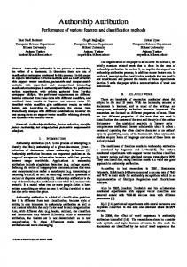
m Figure 1. Classification accuracy results on GA (up) and GB (down) for EDS and kRC ensembles (n=1000) with different values of feature subset size (m). All measures averaged over 50 tries with standard error bars. SVM performance is also indicated for comparison purposes.
These two models were tested on both GA and GB for n=1,000 (i.e., using 1,000 most frequent words of the training corpus to represent the texts) and different feature subset sizes (m=2,3,5,10,15,20,25, and 30). In each case, equal number of base classifiers was used for the two methods (i.e., k=n/m). Figure 1 shows the average ensemble
Authorship Attribution Based on Feature Set Subspacing Ensembles
9
Table 3. Classification effectiveness measures for GB (n=1,000). Accuracy (%) and Mean Reciprocal Ratio of the base classifiers, diversity (entropy) and accuracy (%) of the kRC and EDS ensembles (all measures averaged over 50 tries). m
Base classifiers
kRC Ensemble
EDS Ensemble
2 3 5 10 15 20 25 30
Acc. 16 18 22 29 34 38 41 43
Div. 0.97 0.98 0.96 0.93 0.89 0.85 0.82 0.78
Div. 0.97 0.98 0.97 0.93 0.89 0.86 0.83 0.80
MRR 0.38 0.38 0.39 0.45 0.49 0.52 0.54 0.56
Acc. 94 95 94 94 94 94 93 93
Acc. 99 99 98 97 96 96 95 94
classification accuracy (% of correctly classified test texts) of kRC and EDS ensembles over 50 tries on GA and GB. Standard error bars are also depicted. Surprisingly, ensembles based on small feature subsets (i.e., low m) achieve the best performance for both data sets. Indeed, the performance of the ensembles with m=2 (GA: 90 and GB: 99%, on average) is better from the best reported results for these text corpora (see Table 2) and the SVM baseline. Moreover, the lower the m values, the lower the standard error for EDS. The difference in performance between EDS and kRC is statistical significant (p=0.01) in all cases. A more detailed look at the produced ensembles is given in Table 3, where the average accuracy and MRR of the base classifiers and the diversity among their predictions for the EDS and kRC ensembles (on GB) are shown. As can been seen, there is a trade-off between base classifier accuracy and ensemble diversity. Ensembles based on low m have base classifiers of very low accuracy (recall that random guessing provides accuracy of 10%). However, their diversity is quite high (actually, for m=2 or 3 entropy reaches 1, which means almost randomized error), hence the combination of these poor individual classifiers leads to an accurate ensemble. Notice that the MRR is also reduced with m but to a lower extent in comparison with accuracy. In other words, the true class is ranked in good positions by the base classifiers when they fail to guess it. A significant remark, therefore, is that best ensemble accuracy results are achieved when a large feature set is divided into many small disjoint subsets rather than a few bigger subsets that correspond to better individual base classifiers. Clearly, EDS outperforms SVM for small feature subset size (m