AUTOCORRELATION METHOD FOR ESTIMATION OF DOPPLER PARAMETERS IN FAST-VARYING UNDERWATER ACOUSTIC CHANNELS Yuriy Zakharov and Jianghui Li
Department of Electronics, University of York, York, UK. Yuriy Zakharov, Electronics Department, University of York, Heslington, York, YO10 5DD, UK, Email:
[email protected]
Abstract: In this paper, we propose and investigate a low-complexity technique for estimating the Doppler parameters in fast-varying underwater acoustic channels. This technique can be used in communication systems with periodically transmitted spreadspectrum pilot signals. The known autocorrelation techniques for Doppler estimation suffer from low accuracy in channels fast-varying over the estimation interval. The proposed technique avoids such a problem by introducing a multichannel estimator. The proposed technique not only measures the time compression over the estimation interval, but also the gradient of the time compression, thus allowing more accurate (with timevarying sampling rate) resampling the received signal to compensate for the Doppler distortions. The proposed method is compared with a known autocorrelation technique and the technique based on computing the cross-ambiguity function between the received and pilot signals. The comparison is performed using ocean experiments at short and long distances. The short-range experiment is at a distance of about 3 km with drifting transmitter and receiver (at a speed of 0.5 m/s) and a few discrete multipath components. The long-range experiment is at a distance of 80 km with a transmitter moving at a speed of 6 m/s and a large number of scattered multipath components. The transmitted signal is a pilot-added guard-free OFDM signal. The results demonstrate that, in both the experiments, the proposed technique outperforms the known autocorrelation technique and comparable in the performance with the cross-ambiguity method. The performance improvement is especially significant in the second experiment, where the known autocorrelation method is not capable of providing reliable demodulation of the transmitted data, whereas the proposed technique performs similarly to the crossambiguity method. Keywords: Ambiguity function, autocorrelation, Doppler effect, fast-varying channel, guard-free OFDM, underwater acoustic communication
1. INTRODUCTION In underwater acoustic communications, it is important to accurately estimate the Doppler effect caused by moving transmitter/receiver and reflections from the surface. Relative velocity and acceleration of the transmitter and receiver are usually unavoidable, particularly if both of them are deployed by a surface vessel which is subject to the effects of surface waves and sea currents [1,2,3]. The accurate Doppler estimation is vital for compensating severe Doppler effects. There is a growing interest in the development of Doppler estimation methods which enable compensating the multipath and Doppler effects in time-varying underwater acoustic channels. Various Doppler estimation methods are being actively pursued. Often, the crossambiguity function is used to estimate the Doppler expansion/compression [4,5], in particular, in high-data-rate acoustic communications between rapidly moving platforms, e.g. autonomous underwater vehicles [2]. The cross-ambiguity function estimates can be further refined to improve the estimation accuracy by introducing a residual Doppler shift estimation step [2,5,6,7]. However, the cross-ambiguity function method might be impractical due to its high complexity, as it requires a large number of estimation channels (Doppler sections) and resampling the signal in each Doppler channel [8]. Doppler estimation techniques with lower complexity are required. To reduce the complexity, the time-frequency autocorrelation function of the received signal can be used [9,10], which potentially has significantly fewer estimation channels. The Doppler estimation exploiting the time autocorrelation function (with a single estimation channel) was used, e.g. in [2,8]. However, the known autocorrelation techniques suffer from low accuracy in channels fast-varying over the estimation interval. To alleviate this problem, we propose a Doppler estimate derived from the peak position of the time-frequency autocorrelation. The proposed technique not only measures the time compression over the estimation interval, but also the gradient of the time compression, thus allowing more accurate (with time-varying sampling rate) resampling the received signal to compensate for the Doppler distortions. We apply the proposed technique to guard-free OFDM signals [6,15]. The comparison of the proposed and known techniques, performed using ocean experiments at short (about 3 km) and long (about 80 km) distances with different transmitter and receiver speeds, shows a good performance of the proposed technique, which is comparable to that of the cross-ambiguity method, whereas having significantly lower complexity.
2. TRANSMITTED SIGNAL AND STRUCTURE OF THE RECEIVER We consider transmitting a sequence of the guard-free OFDM symbols [5,6]: 𝑁−1
𝑠𝑝 (𝑡) = ∑ cos (𝜔𝑘 𝑡 + 𝜙𝑝 (𝑘)) , 𝑝 = 1,2,3 … 𝑁𝑝 ,
(1)
𝑘=0
where 𝑁 = 1024 is the number of subcarriers, 𝜔𝑘 = 2𝜋𝑓𝑘 , 𝑓𝑘 = 𝑓𝑐 − 𝐵⁄2 + 𝑘⁄𝑇𝑠 , 𝑓𝑐 is the carrier frequency, 𝑇𝑠 is the symbol duration, 𝐵 = 𝑁⁄𝑇𝑠 is the frequency bandwidth of the signal, and 𝑁𝑝 is the number of OFDM symbols in the transmitted data package. The sequence 𝜙𝑝 (𝑘) represents the phase modulation of subcarriers: √2𝑒 𝑗𝜙𝑝 (𝑘) = 𝑀(𝑘) +
𝑗𝐷𝑝 (𝑘) , where 𝑀(𝑘) ∈ [−1, +1] represents a binary pseudorandom sequence, while 𝐷𝑝 (𝑘) ∈ [−1, +1] represents the information data in the 𝑝th OFDM symbol. The transmitted data are encoded using a 1/2-rate convolutional code; we consider codes represented by the polynomial [3 7], [23 35] and [561 753] in octal [11]. Fig. 1 shows the general structure of the receiver (for more details, please see [6] and [12]). We are interested here in the ‘Doppler estimator’ block. 𝑟(𝑡)
𝑟(𝑖) Front-end Processing
𝑟(𝑛) Resampling & frequency correction
Doppler estimator
Time-domain equalizer
Time-domain equalizer
Frequency -domain equalizer
Frequency -domain equalizer 𝐷(𝑄)
𝐷(𝑄) Combiner & Doppler equalizer
Demodulator
Turbo-iterations
Fig.1 Block diagram of the receiver of guard-free OFDM signals.
3. PROPOSED AUTOCORRELATION DOPPLER ESTIMATOR Fig.2 shows the block diagram of the autocorrelation method. The autocorrelation function is computed on the delay-Doppler shift grid; the autocorrelation is computed over an interval of duration 𝑇𝑠 with a grid of delays in vicinity of the OFDM symbol duration 𝑇𝑠 . The delay step on the grid is chosen as ∆τ = T𝑠 ⁄𝑁𝜏 𝑁 , where 𝑁𝜏 is the time oversampling factor; 𝑁𝜏 can be chosen to be 2 or 4. The Doppler shift is chosen as a predefined fraction of the frequency resolution 𝐵/𝑁𝑓𝑓𝑡 , where 𝐵 is the frequency bandwidth of the OFDM signal and 𝑁𝑓𝑓𝑡 is the length of the Fast Fourier transform (FFT) used for computing the autocorrelation function. The smaller 𝑁𝑓𝑓𝑡 , the simpler the implementation, but with a lower frequency resolution. Typically, 𝑁𝑓𝑓𝑡 is chosen to be the length of one OFDM symbol or twice of it, i.e. 𝑁 or 2𝑁. The refinement of the timing and frequency shift estimates is further applied using the parabolic interpolation (e.g., see [6]). 𝑟(𝑖)
𝑟(𝑛)
Decimation
FFT 𝑒 −𝑗𝛺−𝑁𝑑 𝑛
A(−𝑁𝑑 , : )
FFT
IFFT
|·| A(𝑚, : )
𝑒 −𝑗𝛺𝑚𝑛
Delay 𝑟(𝑛 − 𝑇𝑂𝐹𝐷𝑀 )
FFT
IFFT
|·|
𝑒 −𝑗𝛺𝑁𝑑 𝑛
A(𝑁𝑑 , : )
FFT
Fig.2: Proposed autocorrelation Doppler estimator.
IFFT
|·|
The maximum frequency shift 𝑒 −𝑗𝛺 𝑛 is defined by the maximum speed of the transmitter/receiver. Doppler sections ( 2𝑁𝑑 + 1 sections) of the time-frequency autocorrelation function 𝐴(𝑚, 𝑛) need to cover the whole range of frequency shifts defined by the maximum possible acceleration, 𝑚 = −𝑁𝑑 , … , 𝑁𝑑 , and delays defined by the maximum possible speed. For a wide-band continuous periodic transmitted signal 𝑠0 (𝑡) with the period 𝑇𝑠 , we have: 𝑠0 (𝑡 + 𝑇𝑠 ) = 𝑠0 (𝑡). If a channel is modelled as a delay line with a time-varying delay 𝜏𝑑 (𝑡) , the output of the channel is 𝑠(𝑡) = 𝑠0 (𝑡 − 𝜏𝑑 (𝑡)) . For estimation of parameters of 𝜏𝑑 (𝑡), the autocorrelation function 𝑁𝑑
𝛩⁄2
ρ(τ) =
∫ 𝑠 ∗ (𝑡)𝑠(𝑡 + 𝜏)dt
(2)
−𝛩⁄2
can be used, where 𝛩 is an integration interval. In a channel with a linear variation of delay over time, which is described by a time compression factor, the compression factor can be estimated by searching for the maximum of |𝜌(𝜏)|. The ratio of the peak position 𝑇𝑚𝑎𝑥 of the autocorrelation function to the signal period 𝑇𝑠 can be considered as an estimate of the compression factor. However, this approach provides a limited accuracy when the Doppler compression factor varies over the signal period, i.e. the delay line is described by an equation of a higher order, e.g. if 𝜏𝑑 (𝑡) is a quadratic polynomial. In the fast-varying channels, for estimation of Doppler parameters, instead we can use the following statistics: 𝜃⁄2
ρ(τ, Ω) = ∫ 𝑠 ∗ (𝑡)𝑠(𝑡 + 𝜏)e𝑗Ωt dt .
(3)
−𝜃⁄2
Specifically, the position of the peak of |𝜌(𝜏, Ω)| within the anticipated Doppler range, i.e. [𝑇𝑚𝑎𝑥 , 𝛺𝑚𝑎𝑥 ] = 𝑎𝑟𝑔 𝑚𝑎𝑥|𝜌(𝜏, 𝛺)| , where 𝛺 ∈ [−𝛺𝑚 , 𝛺𝑚 ] and 𝜏 ∈ [𝑇𝑠 − 𝜏𝑚𝑎𝑥 , 𝑇𝑠 + 𝜏𝑚𝑎𝑥 ], allows more accurate estimating the Doppler parameters. To analyse the received signal, we represent the transmitted signal 𝑠0 (𝑡) using the low frequency equivalent 𝑠0 (𝑡) = 𝑠0 (𝑡)𝑒 𝑗𝜔𝑐𝑡 , where 𝑠0 (𝑡) is a low frequency signal, 𝜔𝑐 is a carrier frequency. Then the product 𝑧(𝑡, 𝜏) = 𝑠 ∗ (𝑡)𝑠(𝑡 + 𝜏) involved in the integral in (3) can be represented as 𝑧(𝑡, 𝜏) = 𝑠0∗ (𝑡 − 𝜏𝑑 (𝑡))𝑠0 (𝑡 + 𝜏 − 𝜏𝑑 (𝑡 + 𝜏)) = 𝑠0∗ (𝑡 − 𝜏𝑑 (𝑡))𝑠0 (𝑡 + 𝜏 − 𝜏𝑑 (𝑡 + 𝜏))𝑒 𝑗𝜔𝑐[𝜏𝑑 (𝑡)−𝜏𝑑 (𝑡+𝜏)+𝜏] .
(4)
Taking into account the effects of relative motion of the transmitter/receiver, we use a quadratic polynomial for modelling the time-varying delay: 𝜏𝑑 (𝑡) = 𝑎0 + 𝑎1 𝑡 + 𝑎2 𝑡 2 , where 𝑡 is a time at the transmitter, 𝑎0 is a constant delay, 𝑎1 is the compression factor, 𝑎2 is a factor describing the effect of acceleration. The time 𝑡 + 𝜏𝑑 (𝑡) at the receiver corresponds to the time 𝑡 at the transmitter. Then, the component 𝜏 + 𝜏𝑑 (𝑡) − 𝜏𝑑 (𝑡 + 𝜏) in (4) can be represented as 𝜏 + 𝜏𝑑 (𝑡) − 𝜏𝑑 (𝑡 + 𝜏) = 𝜏 − 𝑎1 𝜏 − 2𝑎2 𝑡𝜏 − 𝑎2 𝜏 2 .
(5)
For 𝛺 = 𝛺𝑚𝑎𝑥 , we can approximately write that 𝑒 𝑗𝜔𝑐[𝜏𝑑 (𝑡)−𝜏𝑑 (𝑡+𝜏)+𝜏] = 𝑒 −𝑗𝛺𝑚𝑎𝑥 𝑡 𝑒 𝑗𝛹 , where 𝛹 is a constant value independent of time 𝑡. We then obtain
𝜔𝑐 𝑇𝑚𝑎𝑥 [1 − 𝑎1 − 2𝑎2 𝑡 − 𝑎2 𝑇𝑚𝑎𝑥 ] = −𝛺𝑚𝑎𝑥 𝑡 + 𝛹.
(6)
From this equation, it follows that 𝛹 = −𝜔𝑐 𝑇𝑚𝑎𝑥 [1 − 𝑎1 − 𝑎2 𝑇𝑚𝑎𝑥 ]. However, the term involving Ψ can be ignored as it does not affect the magnitude |𝜌(𝜏, 𝛺)|. We also obtain that −𝜔𝑐 2𝑎2 𝑇𝑚𝑎𝑥 𝑡 = −𝛺𝑚𝑎𝑥 𝑡, from which we arrive at an estimate of the parameter 𝑎2 : 𝑎̂2 =
𝛺𝑚𝑎𝑥 . 2𝜔𝑐 𝑇𝑚𝑎𝑥
(7)
The fact that the maximum of |𝜌(𝜏, 𝛺)| is achieved at τ = 𝑇𝑚𝑎𝑥 means that for 𝜏 = 𝑇𝑚𝑎𝑥 we can approximately write 𝜏 + 𝜏𝑑 (𝑡) − 𝜏𝑑 (𝑡 + 𝜏) = 𝑇𝑠 , i.e. 𝑇𝑚𝑎𝑥 [1 − 𝑎1 − 2𝑎2 𝑡 − 𝑎2 𝑇𝑚𝑎𝑥 ] = 𝑇𝑠 . The term 2𝑎2 𝑡 represents a problem as it depends on time 𝑡. Since we can 𝜃 𝜃 take an average of the value in the observation interval [− 2 , 2], 𝑎2 𝑡 can be ignored. We can now arrive at 𝑇𝑚𝑎𝑥 [1 − 𝑎1 − 𝑎2 𝑇𝑚𝑎𝑥 ] = 𝑇𝑠 , and the estimate 𝑎1 is given by 𝑇 𝑇 𝛺𝑚𝑎𝑥 𝑎̂1 = 1 − 𝑇 𝑠 − 𝑎2 𝑇𝑚𝑎𝑥 = 1 − 𝑇 𝑠 − 2𝜔 . 𝑚𝑎𝑥
𝑚𝑎𝑥
𝑐
The estimates of the parameters 𝑎1 and 𝑎2 , obtained in the proposed autocorrelation Doppler estimator, are used for approximation of the delay 𝜏𝑑 (𝑡) for resampling the received signal (see Fig. 1).
4. EXPERIMENT In order to verify the effectiveness of the proposed autocorrelation method, the receiver with different Doppler estimation methods was applied to signals from two ocean experiments. We compare the proposed (multiple Doppler sections) autocorrelation method, the known (single Doppler section) autocorrelation method and the crossambiguity method. In the first experiment, the guard-free OFDM symbols at the carrier frequency 768 Hz with a frequency bandwidth of 256 Hz were transmitted at a distance of 3 km from a drifting transmitter to a drifting omnidirectional receiver; the relative speed was about 0.5 m/s. The depth of both the transmitter and receiver were at 200 m. The BER performance of the receivers with the three Doppler estimators is shown in Table 1. Note that, since in this experiment the speed and acceleration of the transmitter/receiver were low, we would expect a similar performance for the single-channel and multichannel autocorrelators. It can be seen that the proposed estimator guarantees the performance comparable to that of the cross-ambiguity method, and it still outperforms the single-channel autocorrelation method. Thus, even in this low-speed case, the proposed estimator results in the performance improvement. Doppler estimator Code [3 7] Code [23 35] Code [561 753] 5 Cross-ambiguity function 0 0 2.4 10 3 3 Single-channel autocorrelation 1.0 10 1.0 10 1.4 103 Multiple channel autocorrelation 0 0 4.1 105 Table 1: BER performance of the receiver with different Doppler estimators; low speed.
In the second experiment, the guard-free OFDM symbols at the carrier frequency 3072 Hz with a frequency bandwidth of 1024 Hz were transmitted at a distance from 80 to 78 km. The transducer was towed at a speed of 12 knots at a depth of 200 m, whereas the drifting omnidirectional hydrophone was positioned at a depth of 400 m. During the communication session, 373 OFDM symbols were received. Fig. 3 shows fluctuations of the channel impulse response in the experiment. The BER performance of the receiver with the three Doppler estimators for this experiment is shown in Table 2. It can be seen that the proposed estimator guarantees a performance similar to that of the crossambiguity method and it is significantly better than that provided by the single-channel autocorrelator. The low performance of the single channel autocorrelator can be explained using the two plots in Fig. 4. The left plot shows an example of the autocorrelation on the delay-Doppler grid with the autocorrelation maximum in the central (#5) Doppler channel. This is a case, where the single-channel autocorrelator provides a performance similar to that of the multi-channel autocorrelator. The right plot shows an example with the maximum in a non-central Doppler channel, i.e., this example corresponds to a high transmitter/receiver acceleration. As a result, the receiver with the single-channel autocorrelator is not capable of providing an accurate Doppler estimate and, consequently, the detection performance is poor.
Fig. 3: Fluctuations of the channel impulse response in the second (long-distance) experiment. Doppler estimator Code [3 7] Code [23 35] Code [561 753] 3 Cross-ambiguity function 4.5 10 8.5 104 2.0 105 Single-channel autocorrelation 0.30 0.34 0.37 3 4 0 Multiple channel autocorrelation 9.2 10 4.8 10 Table 2: BER performance of the receiver with different Doppler estimators; high speed.
Fig. 4: Examples of the time-frequency autocorrelation function in the second (longdistance, high speed) experiment. The left plot shows an example with the autocorrelation maximum in the central (#5) Doppler channel. The right plot shows an example with the maximum in a non-central Doppler channel; this is a case where the single-channel autocorrelator is not capable of providing an accurate Doppler estimate.
5. CONCLUSIONS
In this paper, we have proposed and investigated a new (multi-channel) autocorrelation method for Doppler estimation in fast-varying underwater acoustic channels. The proposed technique not only measures the time compression over the estimation interval, but also the gradient of the time compression, thus allowing more accurate (with timevarying sampling rate) resampling the received signal to compensate for the Doppler distortions. The proposed method has been compared with a known (single-channel) autocorrelation technique and the technique based on computing the cross-ambiguity function between the received and pilot signals. The results demonstrate that the proposed technique outperforms the known autocorrelation technique and it is comparable in the performance with the cross-ambiguity method in both the experiments. The performance improvement compared to the single channel autocorrelation technique is especially significant in the second experiment with a fast moving transmitter, where the known autocorrelation method is not capable of providing reliable demodulation of the transmitted data, whereas the proposed technique provides a high detection performance.
REFERENCES [1] C. Liu, Y. V. Zakharov, and T. Chen, Doubly Selective Underwater Acoustic Channel Model for a Moving Transmitter/Receiver, IEEE Transactions on Vehicular Technology, vol. 61, no. 3, pp. 938-950, 2012. [2] B. S. Sharif, J. Neasham, O. R. Hinton, and A. E. Adams, A computationally efficient Doppler compensation system for underwater acoustic communications. IEEE Journal of Oceanic Engineering, vol. 25, no. 1, pp. 52-61, 2000. [3] J. S. Dhanoa and R.R. Ormondroyd, Combined differential Doppler and time delay compensation for an underwater acoustic communication system, in OCEANS’02, MTS/IEEE, pp. 581-587, 2002. [4] B. S. Sharif, J. Neasham, O. R. Hinton, and A. E. Adams, Doppler compensation for underwater acoustic communications, OCEANS'99 MTS/IEEE. Riding the Crest into the 21st Century, vol. 1, pp. 216-221,1999. [5] Y. V. Zakharov and V. Kodanev, Experimental study of an underwater acoustic communication system with pseudonoise signals, Acoustical Physics, vol. 40, No. 5, pp. 707-715, 1994. [6] Y. V. Zakharov, A. K. Morozov, OFDM Transmission Without Guard Interval in Fast-Varying Underwater Acoustic Channels, IEEE Journal of Oceanic Engineering, pp. 1-15, 2014. [7] M. Johnson, L. Freitag, and M. Stojanovic, Improved Doppler tracking and correction for underwater acoustic communications, IEEE International Conference on Acoustics, Speech and Signal Processing, 1997, ICASSP-97, vol. 1, pp. 575-578, 1997. [8] B. S. Sharif, J. Neasham, O. R. Hinton, A. E. Adams and J. Davies, Adaptive Doppler compensation for coherent acoustic communication, IEE Proceedings-Radar, Sonar and Navigation, vol. 147, no. 5, 2000. [9] G. Jourdain, Characterization of the Underwater Channel: Application to Communication, Berlin Heidelberg, Germany: Springer-Verlag, vol. F1, NATO ASI Series, pp. 197-209, 1983. [10] S. M. Kay, and S. B. Doyle, Rapid estimation of the range-Doppler scattering function, IEEE Transactions on Signal Processing vol. 51, no. 1, pp. 255-268, 2003. [11] J. G. Proakis, Digital Communication, McGraw-Hill, Third Edition, 1995. [12] Y. Zakharov and A. Morozov, “Adaptive sparse channel estimation for guardfree OFDM transmission in underwater acoustic channels”, in Proceedings of UAC2013, June 2013, Corfu, Greece.